Tops and Writhing DNA

Abstract

The torsional elasticity of semiflexible polymers like DNA is of biological significance. A mathematical treatment of this problem was begun by Fuller using the relation between link, twist and writhe, but progress has been hindered by the non-local nature of the writhe. This stands in the way of an analytic statistical mechanical treatment, which takes into account thermal fluctuations, in computing the partition function. In this paper we use the well known analogy with the dynamics of tops to show that when subjected to stretch and twist, the polymer configurations which dominate the partition function admit a local writhe formulation in the spirit of Fuller and thus provide an underlying justification for the use of Fuller’s “local writhe expression” which leads to considerable mathematical simplification in solving theoretical models of DNA and elucidating their predictions. Our result facilitates comparison of the theoretical models with single molecule micromanipulation experiments and computer simulations.

1 Introduction

DNA, which carries the genetic code of living organisms is a semiflexible polymer. The elastic properties of DNA are relevant to a number of biological processeswang . Twist rigidity plays an important role in packaging metres of DNA efficiently in the tiny volume of the cell nucleus, just a few microns across. This involves DNA-histone association which makes use of supercoiling in an essential way. The process of DNA transcription can generate and be regulated by supercoilingstrick .

To understand such effects, there have been single molecule experimentsstrick which pull and twist DNA molecules to probe their elastic properties. However, the interpretation of these experiments has been hindered by a lack of understanding of the geometry of writhe, the twisting of a DNA backbone. The writhe of a DNA polymer configuration, viewed as a space curve, is a nonlocal quantity which has subtle geometric and topological properties. The nonlocality of the writhe makes it cumbersome to use in analytical or computational work markotwist ; volo ; maggs ; roseu ; swig ; berpri ; canturck . This paper is devoted to understanding the writhe for configurations which dominate the partition function: those close to the minima of the energy functional. More precisely, we show that for the stable solutions of the Euler-Lagrange equations (local minima of the energy) the writhe can be expressed as a local integral. This result can be used to develop an analytical approach to the computation of the partition function.

The most popular theoretical model for describing semiflexible polymers is the worm-like-chain (WLC)marko . The WLC is the “ harmonic oscillator” in the field of semiflexible polymers: it is a simple model which deftly captures much of the physics. Given the importance of semiflexible polymers to biology, from lipids to cytoskeletons to DNA, the WLC deserves to be much better understood than it presently is. Two extreme situations are relatively well understood. If the polymer is highly stretched and nearly straight, one can use perturbation theory about the straight line to calculate its elastic propertiesnelson ; sinha ; freesinha ; samsupabhi ; abhi . Treatments also exist volo in the opposite extreme when the polymer is wrung so hard that it buckles and forms plectonemic structureskamien , which are stabilised by the finite thickness of the polymer. The transitional regime where the polymer is neither straightsinha ; nelson nor plectonemickamien is the subject of this paper. Perturbation theory about the straight line is not applicable and the simplifications that arise from the energy dominated plectonemic regime do not obtain. We address this regime by finding the minima of the energy functional in the partition function. These minima come in two families- the straight line family and the “writhing” family, which deviates considerably from the straight line. We study these configurations which dominate the partition function in the transitional regime. We show that these curves admit a local writhe formulation. This leads to a considerable simplification of the theory.

The paper is organized as follows. Sec $II$ presents a recapitulation of the geometrical notion of writhe of a simple space curve and how it can be applied to understand DNA elasticity. Sec $III$ deals with the mechanics of semiflexible polymers using the classical mechanics of a topkirchoff . We prove our main result here: the polymer configurations which dominate the partition function admit a local writhe formulation. Brief remarks regarding perturbations about the saddle point and stability are made in Sec $IV$. We end with some concluding remarks in Sec. $V$.

2 Geometry

In this section we deal with the essential geometric notions that determine the twist elastic properties of linear molecules like DNA. This section is a recapitulation of some material that has been presented earlier samsupabhi and is being summarised here for the reader’s convenience. The experiments of Strick et al strick are done on an open segment of DNA which is attached to a glass slide at one end and a magnetic bead on the other. The bead is pulled to stretch the molecule and turned to “wind it up” and induce supercoiling. For mathematical convenience, we close the open segment of DNA by a reference ribbon (a ribbon is a framed space curve) in a manner described in samsupabhi (see Figs. 4 and 5 of Reffuller and references therein). The fixed reference loop (called the passive part) is held fixed and our discussion concerns only the active part of the curve. (It is also possible to choose the reference ribbon as coming in from infinity along the ${\hat{z}}$ direction and going off to infinity along the ${\hat{z}}$ direction. The precise choice of reference does not matter.)

The basis of the analysis of DNA supercoiling is the celebrated relation calugeranu ; white ; fuller1 ; fuller :

$$Lk=Tw+Wr$$ (1)

which relates the applied link (the number of times the bead is turned in the experiment) to the twist (the twisting of the polymer about its tangent vector) and the writhe (the bending of the tangent vector). The problem neatly splits fuller ; samsupabhi into two parts: a relatively straightforward (local) description of the twist elasticity, and the somewhat harder (nonlocal) treatment of the writhe.

The writhe is a non-local quantity defined on closed simple curves: Let the arc length parameter $s$ range over the entire length $L_{0}$ of the closed ribbon (real ribbon $+$ reference ribbon) and let us consider the curve ${\vec{x}}(s)$ to be a periodic function of $s$ with period $L_{0}$. Let ${\vec{R}}(s,\sigma)={\vec{x}}(s+\sigma)-{\vec{x}}(s)$. We write ${\hat{t}}(s)=\frac{d{\vec{x}}}{ds}$ for the unit tangent vector to the curve. Since the curve ${\vec{x}}(s)$ is simple, ${\vec{R}}(s,\sigma)$ is non-vanishing for $\sigma\neq 0,L_{0}$ and the unit vector ${\hat{R}}(s,\sigma)$ is well-defined. It is easily checked that as $\sigma\rightarrow\{0,L_{0}\},$ ${\hat{R}}\rightarrow\{{\hat{t}},{-\hat{t}}\}$ respectively. The Călugăreanu-White writhe is given bydennis ; calugeranu ; white ; fuller1 ; fuller

$${\cal W}_{CW}=\frac{1}{4\pi}\oint_{0}^{L_{0}}ds\int_{0+}^{L_{0}-}d\sigma[\frac{d{\hat{R}(s,\sigma)}}{ds}\times\frac{d{\hat{R}(s,\sigma)}}{d\sigma}]\cdot{\hat{R}.}$$ (2)

The non-locality of ${\cal W}_{CW}$ makes it difficult to handle analytically. However, the key point to note is that variations in ${\cal W}_{CW}$ are local fuller ; fuller1 . Let ${{\cal C}}(\alpha)$ be a family of polymer configurations parametrised by $\alpha$ of simple closed curves with writhe ${\cal W}_{CW}(\alpha)$. Taking the ${\alpha}$ derivative of Eq. (2) (which now depends parametrically on $\alpha$) we find that the resulting terms can be rearranged to give

$$\frac{d{\cal W}_{CW}}{d\alpha}=\frac{1}{2\pi}\oint_{0}^{L_{0}}ds[\frac{d{\hat{t}}}{ds}\times\frac{d{\hat{t}}}{d{\alpha}}]\cdot{\hat{t},}$$ (3)

which clearly has the interpretation of the rate at which ${\hat{t}}(s,\alpha)$ sweeps out a solid angle in the space of directions. Note that Eq.(3) which gives the change in writhe is a single integral bouchiat ; fain and therefore a local, additive quantity. This can be expressed as a sum of the changes in the active parts of the curve and therefore, since the passive part is unchanged in the variation, the change in writhe is entirely due to the active part $0\leq s\leq L$, where $L$ is the contour length of the active part of the polymer. Eq. (3) can be rewritten as:

$$\frac{d{\cal W}_{CW}}{d\alpha}=\frac{1}{2\pi}\frac{d{\Omega}({\alpha})}{d\alpha}=\frac{1}{2\pi}\int_{0}^{L}ds[{\hat{t}}\times\frac{d{\hat{t}}}{ds}]\cdot\frac{d{\hat{t}}}{d{\alpha}}$$ (4)

where $\Omega$ is the solid angle enclosed by the oriented curve {${\hat{t}}(s)|0\leq s\leq L$} on the unit sphere of tangent directions as $s$ goes from $0$ to $L$ kamien . Note that $\Omega$ is only defined modulo $4\pi$: for a solid angle $\Omega$ to the left of the oriented curve ${\hat{t}}(s)$ is equivalent to a solid angle $(4\pi-\Omega)$ to the right. $d\Omega/d\alpha$ is, however, well defined and local. Integrating Eq. (4) we arrive atfuller ; fuller1 :

$${\cal W}_{CW}({\alpha})=\frac{1}{2\pi}{\Omega}-1+2n$$ (5)

where $n$ is an arbitrary integer. The constant of integration is fixed by noting that the writhe of a simple planar curve vanishes (Eq.2).

There is a quantity one can construct from the writhe which is well defined on all curves (not just simple ones)

$$w({{\cal C}})=exp[i\pi{\cal W}_{CW}({{\cal C}})]=-exp[{i\Omega}/2]$$

is a complex number of modulus unity which we call the wreathe. When a curve is passed through itself, ${\cal W}_{CW}$ jumps by $2$, but the wreathe is unchanged. We can therefore smoothly extend $w$ to all closed curves including non-simple curves. Unlike the writhe, the wreathe $w$ is a local quantity. The wreathe can be exploited to define a new quantity, the Fuller “writhe” fuller ; fuller1 for a class of curves. (Readers familiar with the geometric phase in quantum mechanics Berry:1984jv ; shapere ; js ; samsup will recognise the relation between the wreathe, the Fuller writhe, the Berry phase and the Pancharatnam connection.) Let us fix a direction (say $-{\hat{z}}$, which we call “south”) and define “south avoiding” curves to be those for which the tangent vector never points south . The Fuller “writhe” is defined for south avoiding curves. Let us define the “wreathe angular velocity” ${\cal A}_{\alpha}=-iw^{-1}{\frac{dw}{d\alpha}}=1/2d\Omega/d\alpha$ on the family of curves ${\cal C}_{\alpha}$ parametrised by $\alpha$. Let us choose a fiducial curve ${{\cal C}_{*}}$, of length $L$, whose tangent vector is identically north pointing. We take this as a standard for the “active part” of the curve, the “passive part”, of course being held fixed in the discussion. Observe that all south avoiding curves are deformable to the fiducial curve ${{\cal C}_{*}}$. One simply deforms the tangent vector ${\hat{t}}(s)$ along the unique shorter geodesic connecting ${\hat{t}}(s)$ to the north pole. We now define the “Fuller writhe” as

$${\cal W}_{F}=1/\pi\int_{{\cal C}_{*}}^{{\cal C}}d\alpha{\cal A}_{\alpha}-1.$$

Writing the unit tangent vector as ${\hat{t}}=(\sin{\theta}\cos{\phi},\sin{\theta}\sin{\phi},\cos{\theta})$, $\int_{0}^{1}{d{\alpha}\frac{d\Omega}{d\alpha}}$ can be written as $\int{ds\frac{d{\phi}}{ds}(1-\cos{\theta})}$ for all curves for which the tangent vector never points towards the south pole of the sphere of tangent directions. We can therefore write bouchiat ; fain a local writhe formula on such curves which we call “south avoiding curves”:

$${\cal W}_{F}={\frac{1}{2\pi}}\int{ds{(1-\cos{\theta}){\frac{d{\phi}}{ds}}}}-1.$$ (6)

While (Eq. 6) is expressed in local co-ordinates on the sphere, it has a clear geometric meaning: $2\pi(1+{\cal W}_{F})$ is equal to the solid angle swept out by the unique shorter geodesic connecting the tangent vector ${\hat{t}}$ to the north pole. This definition is explicitly not rotationally invariant, since it uses a fixed fiducial curve ${{\cal C}_{*}}$ and singles out a preferred direction.

To summarise, ${\cal W}_{CW}$ is defined on all self-avoiding curves, ${\cal W}_{F}$ on all south avoiding curves. When a curve passes through itself, ${\cal W}_{CW}$ jumps by two and when the tangent vector to a curve swings through the south pole, ${\cal W}_{F}$ jumps by two units. The writhe is a real number which has both geometric and topological information. The topological part is the integer part of $\frac{{\cal W}_{CW}}{2}$ and the geometric part is the fractional part of $\frac{{\cal W}_{CW}}{2}$. The geometric part is completely captured by wreathe but the topology is lost since wreathe is insensitive to changes in writhe by $2$ units. From the definitions it is clear that on a family of curves ${\cal C}_{\alpha}$ parametrised by $\alpha$,

$$-i{\frac{{w}^{-1}}{\pi}}{\frac{dw}{d\alpha}}=\frac{d{\cal W}_{CW}}{d\alpha}=\frac{d{\cal W}_{F}}{d\alpha}$$ (7)

So, continuous changes in writhe are the same whether measured by ${\cal W}_{CW},{\cal W}_{F}$ or $w$. We have adjusted the reference ribbon and the definition of Fuller writhe so that these two notions of writhe ${\cal W}_{CW}$ and ${\cal W}_{F}$ agree on the reference curve. Note that $w$ is well-defined on all curves. For a closed circuit of curves $\{{\cal C}_{\alpha},(0\leq\alpha\leq 1),{\cal C}_{0}={\cal C}_{1}\}$, we have the “closed circuit theorem” samsupabhi : In a closed circuit of curves, the total number of south crossings and self crossings (both counted with sign) are the same. This follows easily by integrating (Eq. 7) along a closed circuit.

This definition of “Fuller writhe” is motivated by a Theorem of Fullerfuller ; fuller1 , which uses a reference curve and states precise conditions (which are frequently misunderstoodneukirch ) under which the writhe difference between the two curves can be written as a local integral. Under deformations of the reference curve which are both south avoiding and self avoiding (we follow neukirch in calling these “good deformations”), Eq. (7) implies that the equality ${\cal W}_{CW}={\cal W}_{F}$ is maintained. These deformations are the ones which satisfy the conditions of Fuller’s theorem [Eq. 6.4 in Ref. fuller ]. We refer to curves which can be reached from the reference curve by “good deformations” as “good curves”.

To avoid misunderstanding, we remark that the “Fuller writhe” is a distinct quantity from ${\cal W}_{CW}$ and is not equal to the Călugăreanu-White writhe. This is obvious since the first is local, while the second is not. Strictly speaking Fuller only defines a local writhe on “good curves”, where it is equal to the CW writhe. We find it convenientsamsupabhi to extend Fuller’s defintion to all south avoiding curves and not just “good curves”. On “good curves”, the two notions of writhe agree and we have ${\cal W}_{F}$ equal to ${\cal W}_{CW}$, but the two quantities are different in general. The main claim of samsupabhi is that “good curves” dominate the partition function in a region of the parameter space. We will substantiate this claim in the next section by identifying the dominant configurations that contribute to the partition function in a saddle point approximation and showing that they are “good curves”.

In the high force regionsinha ; nelson this point is obvious since the polymer fluctuates about the straight line configuration which is a good curve. The content of the following section is that even at lower forces (or at large torques, close to buckling) when the polymer is far from straight, the minima of the energy are “good curves”. The analysis involves a combination of mechanics, geometry and topology.

3 Mechanics

Semiflexible biopolymers like DNA are subject to thermal fluctuations in a cellular environment. Therefore the natural theoretical framework for studying the elastic properties of such systems is statistical mechanics, which involves a competition between energy and entropy. In the experiment, one controls the force $F$ on the bead and the link $Lk$, the number of times the bead is turned. This brings up the theoretical problem of computing the partition function $Z(F,Lk)$, the number of configurations (counted with Boltzmann weight) of the ribbon which have a given link (the link distribution). We know that the link distribution is a convolution of the writhe distribution and the twist distributionbouchiat ; sinha . The latter is a simple Gaussian integral, which is easily computed. The real problem is to compute the writhe distribution of an inextensible curve. By simple transformations samsupabhi the problem of determining the link distribution of an inextensible ribbon can be reduced to computing the writhe distribution of a space curve. The partition function to be computed is

$$Z(F,W)=\sum_{\it{\cal C}}{exp[-{\cal E}({\cal C})/k_{B}T]\delta({\cal W}_{CW}-W)}$$ (8)

where $F$ is the force, ${\cal E}({\cal C})$ the energy (defined below in eq.(9)) and ${\cal W}_{CW}$ is the writhe. The sum is over all allowed configurations of the polymersamsupabhi . We expect the sum to be dominated by configurations which minimise the energy functional. Configurations near the minimum will also contribute due to thermal fluctuations. We first do a purely classical elastic analysis taking only the energy into account, while ignoring the entropyfuller1 ; love ; maddockspnas ; fain . This allows us to draw on physical intuition derived from the elasticity of beams, cables, telephone cords and ribbons and paves the way for a fuller treatment which incorporates thermal fluctuations around the classical solutions. We analyze the classical elasticity of a torsionally constrained stretched semiflexible polymer.

The problem can be reduced to minimizing the energy (we use a dot for the $s$ derivative, it reinforces the analogy kirchoff with the dynamics of tops)

$${\cal E}[\hat{t}(s)]=\frac{1}{2}\int_{0}^{L}\dot{\hat{t}}.\dot{\hat{t}}ds-\int_{0}^{L}\vec{F}.\hat{t}ds$$ (9)

of a space curve $\vec{x}(s)$ whose tangent vector is $\hat{t}(s)=\frac{d\vec{x}}{ds}$, subject to a writhe constraint

$${\cal W}_{CW}=W$$ (10)

where, ${\cal W}_{CW}$, the Călugăreanu-White writhe has been defined earlier. The tangent vector $\hat{t}(s)$ is varied subject to the boundary conditions $\hat{t}(0)=\hat{t}(L)=\hat{z}$ fixing the tangent vector to the curve at both ends. As mentioned clearly in nelson ; sinha ; samsupabhi , the full problem involving the link distribution (with finite twist elasticity) can be reduced to computing the writhe distribution, which is essentially the limit of infinite twist rigidity ($C\rightarrow\infty$).

Using the method of Lagrange multipliers we arrive at

$$\delta{\cal E}({\cal C})=2\pi\tau\delta{\cal W}_{CW}$$ (11)

where $2\pi\tau$ is a Lagrange multiplier. $\tau$ can be physically interpreted as a torque. The variation in the energy $\delta{\cal E}$ is given by

$$\delta{\cal E}=-\int_{0}^{L}(\ddot{\hat{t}}+\vec{F})\cdot\delta{\hat{t}}$$ (12)

The variation of ${\cal W}_{CW}$ (as explained earlier (4)) is a local quantity

$$\delta{\cal W}_{CW}=\frac{1}{2\pi}\int_{0}^{L}[{\hat{t}}\times\dot{\hat{t}}]\cdot\delta{\hat{t}}ds$$ (13)

and the Euler-Lagrange (E-L) equations are

$$-\ddot{\hat{t}}-{\vec{F}}=\tau({\hat{t}}\times{\dot{\hat{t}}})-\gamma{\hat{t}},$$ (14)

where the term $\gamma{\hat{t}}$ arises since $\delta{\hat{t}}\cdot{\hat{t}}=0$. Note that the E-L equations are local differential equations rather than the nonlocal integral equations that one may have expected from the variation of a non local quantity ${\cal W}_{CW}$. Thus, the variations of writhe ${\cal W}$ are local. As we will see, this is the key idea that allows us to prove that “good curves” dominate the partition function.

The statics of a twisted beam (or cable or DNA) is formally similar to the dynamics of a heavy symmetrical top, a fact that has been well known since Kirchoffkirchoff . The analogy is useful for integrating the Euler-Lagrange equations. We use quotes for the analogous top quantities. The “kinetic energy” is given by $T=\frac{1}{2}{\dot{\hat{t}}}\cdot\dot{\hat{t}}$ and the “potential energy” is $V={\vec{F}}\cdot{\hat{t}}$. The total “energy”

$${\cal H}=T+V=\frac{1}{2}(\dot{\theta}^{2}+\sin^{2}\theta\dot{\phi}^{2})+F\cos\theta$$ (15)

is a “constant of the motion” as is the $z$ component of the “angular momentum”

$$J_{z}=({\hat{t}}\times\dot{\hat{t}})_{z}-\tau{\hat{t}}_{z}=\sin^{2}\theta\dot{\phi}-\tau\cos\theta,$$ (16)

where we have introduced the usual polar coordinates on the space of tangent vectors ${\hat{t}}=(\sin{\theta}\cos{\phi},\sin{\theta}\sin{\phi},\cos{\theta})$. Using these “constants of the motion” we reduce the problem to quadratures as described in goldstein . The basic equations are

$$\frac{\dot{\theta}^{2}}{2}={\cal H}-F\cos\theta-\frac{(J_{z}+\tau\cos\theta)^{2}}{2\sin^{2}\theta}$$ (17)

$$\dot{\phi}=\frac{J_{z}+\tau\cos\theta}{\sin^{2}\theta}.$$ (18)

Setting $u=\cos\theta$, we find that

$${\dot{u}}^{2}=f(u)$$ (19)

where $f(u)$ is a cubic polynomial in $u$. Our boundary conditions imply that $\theta=0$ is a point on the solution. Since ${\dot{\theta}}^{2}$ has to be finite at $\theta=0$, we have $J_{z}=-\tau$. The form of $f(u)$ simplifies to

$$f(u)=(1-u)[2({\cal H}-Fu)(1+u)-\tau^{2}(1-u)].$$ (20)

(18) can be rewritten as

$$\dot{\phi}=\frac{-\tau}{1+u}.$$ (21)

From (17) we also find that ${\cal H}\geq F$, else ${\dot{\theta}}^{2}$ would have to be negative at $\theta=0$. We see that $f^{\prime}(u)|_{u=1}=-4({\cal H}-F)\leq 0$ at $u=1$. At $u=-1$, $f(-1)=-4\tau^{2}\leq 0$ and so $f(u)$ has one physical root at $u=1$ and the other at $u_{0}$ between $-1$ and $1$: $-1\leq u_{0}\leq 1$. The third root $u_{1}$ is generally (except for $u_{1}=\pm 1$) outside the physical range and $u_{1}>1$ for positive force and $u_{1}<-1$ for negative force. Since $f(u_{0})=0$, we find from (20) the useful relation

$$\tau^{2}=\frac{2({\cal H}-Fu_{0})(1+u_{0})}{1-u_{0}}$$ (22)

The “motion” is confined between the turning points $1$ and $u_{0}$: $u_{0}\leq u\leq 1$. We write $u_{0}=\cos{\theta_{0}}$, where $\theta_{0}$ is the turning point for $\theta$. Just as in the top problem, we find that the solution $u(s)$ is periodic with a period given by

$$P=2\int^{1}_{u_{0}}\frac{du}{\sqrt{f(u)}}.$$ (23)

Because of the boundary conditions, we have $L=nP$, where $L$ is the length of the polymer and $n$ is an integer. $L$ and $n$ fix the integration constant ${\cal H}$. We will see in the next section that solutions with $n>1$ are not minima of the energy. We therefore restrict ourselves to $n=1$. Our interest is solely in stable solutions, that is local minima of the energy.

General solutions to these equations can be found in terms of elliptic functions but a pedestrian approach gives more immediate insight. The simplest solution is the straight line $u(s)=1$ for all $s$, which solves the E-L equations (14) for all $F,\tau$ with $F={\cal H}$ for any $L$. However, the straight line cannot accommodate writhe and we have to look at the “writhing family” of solutions parametrised by $F,\tau$. These start from $u(0)=1$ at $s=0$, and have a turning point at $s=s_{0}$ ($u(s_{0})=u_{0}$) and return to $u=1$ at $P=2s_{0}=L$. These solutions can be explicitly written down in terms of elliptic functions and vary continuously with $\tau$ in the allowed range $|\tau|<\sqrt{4F}$. Integrating (Eqs. 17,21) gives $(u(s),\phi(s))$ which gives us the solution to the E-L equations ${\hat{t}}(s)$.

From the “top” point of view, ${\hat{t}}(s)$ is the solution. However, in polymer physics, ${\hat{t}}(s)$ is only a convenient way of describing the polymer configuration ${\vec{x}}(s)$, which is given by

$${\vec{x}}(s)=\int_{0}^{s}ds^{\prime}{\hat{t}}(s^{\prime})$$ (24)

The use of ${\hat{t}}(s)$ rather than ${\vec{x}}(s)$, in the variational problem (Eq. 9) leads to a considerable simplification, since the equations of motion are second order rather than fourth order. However, there is a price to be paid. After solving for the “tantrix” ${\hat{t}}(s)$ (plotted in a special case in Fig. 1), we still have to integrate (Eq. 24) to produce the actual polymer configuration ${\vec{x}}(s)$, (Fig. 2) in real space.

Figure 1: The black curve (tangent indicatrix) traced on the unit sphere (green online) by the unit tangent vector to a long polymer for a force $F=.11$ and torque $\tau=.4$. The dots (in red online) indicate the tips of the unit vectors ${\vec{V}}$ (marked V) and ${\vec{z}}$ (marked N for North).

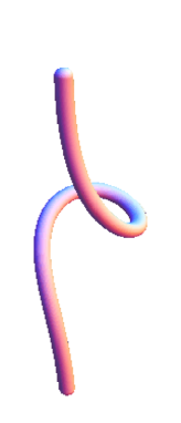
Figure 2: Figure shows the polymer configuration in real space for the same parameters as Fig. 1. The curve has been thickened, shaded and truncated for easy three dimensional visualisation.

In the polymer context it is meaningful to ask: does this configuration intersect itself? Such a question is not significant for tops. Nevertheless, as we will see, the motion of a heavy symmetrical top helps us answer this question.

We prove the main result of this paper: all stable solutions of the E-L equations are “good curves”in the sense of the last section. For the straight line family, the result is obviously true since the straight line is the reference curve. The effort here is showing that all stable members of the writhing family $\hat{t}(s)$ parametrised by $(F,\tau)$ are “good curves”. To do this we prove that the writhing family is nowhere self intersecting or south pointing for $-1<u_{0}\leq 1$. Since $u_{0}=1$ is the straight line ${\hat{t}}(s)={\hat{z}}$, which we take as the reference curve, this proves that the writhing family can be deformed (via a deformation of the parameter $u_{0}$) to the reference curve by “good” deformations and the result follows. Below, we explicitly exclude the case $u_{0}=-1$, which will be treated separately in the next section.

It is evident that the writhing family is nowhere south pointing for $-1<u_{0}\leq 1$ since the turning point $\theta_{0}<\pi$ and the tangent vector ${\hat{t}}(s)$ never points to the south pole. To prove that the writhing family is nowhere self intersecting requires considerably more work. The proof consists of finding a direction ${\vec{V}}$ along which the tangent vector ${\hat{t}}$ to the polymer has positive component. This implies that the polymer never bends back to intersect itself. The proof uses the E-L equations in an essential way but does not rely on the explicit form of the solution.

We first orient our axes by rotating about the $z$ axis so that $\phi(s_{0})=0$ and the tangent vector ${\hat{t}}(s)=(\sin{\theta(s)}\cos{\phi(s)},\sin{\theta(s)}\sin{\phi(s)},\cos{\theta(s)})$ lies in the $x-z$ plane at the turning point. Consider for each $u_{0}=\cos{\theta_{0}}$ the constant ($s$ independent) unit vector $\vec{V}=(-\cos\theta_{0},0,\sin\theta_{0})$. and the function

$$g(s)={\hat{t}}(s)\cdot\vec{V}.$$

Note that the function $g(s)$ is symmetric about $s=s_{0}$ within the period $0\leq s\leq 2s_{0}=P=L$. We show that a) either $g(s)$ vanishes identically or b) $g(s)>0$ for all $s\neq s_{0}$. We need only consider the range $s_{0}\leq s<2s_{0}$, so that $\theta(s)>0,u(s)<1$. $g(2s_{0})$ is fixed by boundary conditions to be $\sin{\theta_{0}}\geq 0$. The positivity of $g(s)$ immediately implies our central result (see below): The polymer configurations under stretch and torque are such that the tangent vectors to the polymer all lie in one hemisphere of the sphere of tangent directions.

The proof proceeds in several steps.
Step 1: $g(s)$ vanishes at the turning point $s_{0}$ and has a local minimum at $s_{0}$ if it does not vanish identically.
Proof: Remembering that ${\dot{\theta}}=0$ at the turning point, we find

$${\hat{t}}(s_{0})=(\sin{\theta_{0}},0,\cos{\theta_{0}})$$ (25)

and

$${\dot{\hat{t}}}(s_{0})=(0,\sin{\theta_{0}}{\dot{\phi}},0)$$ (26)

from which follows

$$g(s_{0})={\hat{t}}(s_{0}).{\vec{V}}=0$$ (27)

$${\dot{g}}(s_{0})={\dot{\hat{t}}}(s_{0}).{\vec{V}}=0$$ (28)

So $s_{0}$ is a stationary point of $g(s)$. To show that $g(s)$ has a local minimum, we compute ${\ddot{g}(s)}$ using the E-L equations (14) and (21,25,26) to find

$${\ddot{g}(s_{0})}=\sin{\theta_{0}}(\frac{\tau^{2}}{1+u_{0}}-F)$$ (29)

Substituting for $\tau^{2}$ (22) and simplifying gives

$${\ddot{g}(s_{0})}=\frac{\sin{\theta_{0}}}{1-u_{0}}(2{\cal H}-F(1+u_{0}))\geq 0$$ (30)

since ${\cal H}\geq F$. The equality occurs only if $\sin{\theta_{0}}$ vanishes ($u_{0}=\pm 1$) in which case $g(s)$ vanishes identically. $u_{0}=1$ describes a straight line segment, which is the reference curve and therefore a “good curve”. $u_{0}=-1$ has been excluded from consideration. Below we will exclude both cases ($u_{0}=\pm 1$) in which $g(s)$ vanishes identically. This proves that $s_{0}$ is a local minimum of $g(s)$ for ($u_{0}\neq\pm 1$).

Step2: At stationary points of $g(s)$,

$$g(s)u(s)>0$$ (31)

for $s\neq s_{0}$.

Proof of Step 2: Since $\dot{g}(s)=\dot{\hat{t}}.{\vec{V}}=0$ at a stationary point, $\dot{\hat{t}}$ is orthogonal to both ${\vec{V}}$ and $\hat{t}$ and can be written. $\dot{\hat{t}}=A{\vec{V}}\times{\hat{t}}$ for some nonzero $A$. “Angular momentum” and “energy” conservation give us

$$\dot{\hat{t}}.\dot{\hat{t}}=2({\cal H}-Fu)$$ (32)

$$({\hat{t}}\times\dot{\hat{t}})_{z}=-\tau(1-u),$$ (33)

which can be rewritten as

$$|A|^{2}(1-g^{2})=2({\cal H}-Fu)$$ (34)

and

$$A(\sin\theta_{0}-gu)=-\tau(1-u)$$ (35)

In Eq.(34) both sides are positive since $u<1$. Squaring (35) and eliminating $|A|^{2}$ and $\tau^{2}$ between (22,34,35), we find that at a stationary point of $g(s)$, $g(s)$ and $u(s)$ satisfy

$$(\sin\theta_{0}-gu)^{2}<\frac{({\cal H}-Fu_{0})(1+u_{0})}{(1-u_{0})}X(u)$$ (36)

where $X(u)=(1-u)^{2}/({\cal H}-Fu)$ is a strictly decreasing function of $u$ in the range of interest. From $X(u)<X(u_{0})$ for $u>u_{0}$ it follows that

$$(\sin\theta_{0}-gu)^{2}<(\sin\theta_{0})^{2}$$ (37)

which implies (31).

Step3: $s_{0}$ is a global minimum of $g(s)$: $g(s)>0$ for $s\neq s_{0}$.

Proof: note that since $s_{0}$ is a local minimum of $g(s)$ (from Step 1), as $s$ increases from $s_{0}$, $g(s)$ increases from 0 (since $s=s_{0}$ is a minimum). If there are no more stationary points $g(s)$ remains positive and we are through. If the next stationary point occurs at $s_{1}>s_{0}$, $\dot{g}(s)|_{s=s_{1}}=0$ we have $g(s_{1})>0$. It follows from Step 2 that $u(s_{1})>0$. Since $u(s)$ is a monotonic function of $s$ in the range $(s_{0}\leq s<2s_{0})$, we have $u(s)>0$ for $s>s_{1}$ in this range. All minima of $g(s)$ for $s>s_{1}$, therefore have $g(s)>0$ (again using Step 2). It follows that $g(s)>0$ for all $s$ (except the one point $s_{0}$, where $g(s_{0})=0)$. From the symmetry of $g(s)$ it follows that $g(s)$ is positive everywhere except at the turning point ($s_{0}$, where it vanishes).

This immediately implies our main result since if any of the minimum energy configurations intersect themselves, $\vec{x}(s_{1})=\vec{x}(s_{2})$ for $s_{2}>s_{1}$, we have

$$\int^{s_{2}}_{s_{1}}{\hat{t}}(s)\cdot ds=0$$

contracting this equation with $\vec{V}$ gives us

$$\int^{s_{2}}_{s_{1}}g(s)ds=0$$

which is a contradiction since $g(s)>0$ for all $s\neq s_{0}$. We have thus proved that the writhing family does not intersect itself for $-1<u_{0}\leq 1$. Since $u_{0}$ can be continuously deformed to $1$ along the writhing family, we conclude that the family consists of “good curves” which admit a local writhe formulation. We now consider variations around the solutions of the E-L equations to test for stability.

4 Fluctuations around the saddle point

In a saddle point approximation to the partition function the dominant thermodynamic contributions are expected to arise from the global minimum of the energy. We can also expect contributions from local minima due to “metastable” states, when the time scale of the experiment is not large enough to find the true minimum. All minima, local and global will satisfy the E-L equations and so will be among the solutions described in the last section. However, not all solutions to the E-L equations are minima of the energy. There are some configurations which, if perturbed, will go to nearby states of lower energy and decay. These configurations do not contribute significantly to the partition function. To weed these out we need to consider the stability of solutions by perturbing the classical solutions to see if there are neighboring lower energy configurations. (We do not concern ourselves here with zero modes arising from symmetry breaking. They contribute an innocuous multiplicative constant to the partition function.)

For example, we note that solutions with $L=nP$ and $n>1$ are unstable. This is seen by explicitly constructing neighboring configurations of lower energy. Suppose $n>1$ and consider the configuration {$u_{\rm old}(s),\varphi_{\rm old}(s)$} which solves the Euler Lagrange equations. Construct a new configuration

$$\left.\begin{array}[]{cc}u_{\rm new}(s)&=u_{\rm old}(s)\\ \varphi_{\rm new}(s)&=\varphi_{\rm old}(s)\end{array}\right\}{\rm for}\;s\leq P$$ (38)

$$\left.\begin{array}[]{cc}u_{\rm new}(s)&=u_{\rm old}(s)\\ \varphi_{\rm new}(s)&=\varphi_{\rm old}(s)+\alpha\end{array}\right.\;\;{\rm for}\;s\geq P$$ (39)

where $\alpha$ may be an arbitrarily small real number. The new configuration

1. satisfies the boundary conditions,

2. has the same energy as the old one (since the energy is a local integral),

3. has the same writhe as the old one (since changes of writhe are local integrals),

4. is not a solution to the ${\cal E}L$ equations at $s=P$ (because of the break in the curve at this point).

It follows that there are neighboring configurations with lower energy than the old configuration and the same writhe. We conclude that the solutions with $n>1$ are not local minima of the energy. A similar remark applies to the straight line family if the torque exceeds a critical torque $\tau_{c}$ given by $(\tau_{c}/2)^{2}=F+(\frac{\pi}{L})^{2}$, the classical condition for torsional buckling of a rod. This can be directly seen by perturbing the straight line. For $\tau>\tau_{c}$ there are no stable solutions of the Euler Lagrange equations and the polymer must double back on itself and enter the plectonemic regime.

We now turn to a discussion of the exceptional member of the writhing family $(u_{0}=-1)$ characterised by $\tau=0$. Note that as $\tau$ ranges from $-\tau_{c}$ to $\tau_{c}$, the writhing family goes in a closed circuit from the straight line to the straight line. The closed circuit has one south crossing (at $\tau=0$ or equivalently $u_{0}=-1$). From the “closed circuit theorem” samsupabhi , it follows that the circuit must also have one self crossing. Since none of the other members of the writhing family have self intersections, it follows that self crossing must occur at $\tau=0$. Thus the closed circuit has one self crossing and one south crossing, both occuring at the same value of the parameter $\tau=0$. The writhing family curve $\tau=0$ does not belong to the configuration space of either self avoiding or south avoiding models and both ${\cal W}_{CW}$ and ${\cal W}_{F}$ are ill defined. One can expand the configuration space to allow all curves and use a formulation in which energy is minimised for fixed wreathe. It can then be shown by an argument very similar to that given above (38) that the curve is unstable. By rotating the second half of the curve by a small angle $\alpha$ relative to the first, keeping the energy and wreathe the same, we can produce neighboring curves which are not solutions of the E-L equations and can therefore be perturbed to lower their energy.

The writhing family curves in the regime $0<|\tau|<\tau_{c}$, include stable solutions, and we can take into account thermal fluctuations in a Gaussian approximation about the local minimum of energy. Since any stable curve of the writhing family is at a finite distance and energy from south and self intersection, we can expect small fluctuations around the original curve to be “ good curves”. Large fluctuations may lead to “bad curves”, but their contributions to the partition function will be exponentially suppressed by the Boltzmann weight, as made clear by the example of comment , and not affect the statistical predictions of the model. Thus the writhing family can be used as a base for a clean discussion of thermal fluctuations without getting embroiled in the topological subtleties of writhe. Such a treatment goes far beyond perturbation theory around a straight line since the writhing family is far from straight.

To summarize, our analysis shows that there is a range of force and torque relevant to single molecule experiments for which the polymer configuration curves are “good” curves.

5 Conclusion

In this paper we present a classical mechanical approach to biopolymer elasticity based on well known analogies between twisted polymers and tops. Our main result is that the dominant configurations in the partition function are “good curves” in a topological sense. This result permits a local formulation of the writhe and a non perturbative attack on the problem of twist elasticity by incorporating thermal fluctuations around the writhing family. Such an approach is expected to work well in the energy dominated regime, when the polymer is twisted and stretched. In this paper, we have restricted ourselves to the mathematical and conceptual issues regarding the use of writhe. Our main result is useful in further developing the theorypapb . Applying these ideas to the WLC leads to detailed predictions about the statistical mechanical behaviour of twisted stretched polymers. These will be described elsewhere.

The experiments of Strick et al strick have been theoretically analysed by Nelson nelson and Bouchiat and Mezard bouchiat . The analysis of Nelson is perturbative about the high force limit (see also sinha ) and not controversial. However, Bouchiat and Mezard bouchiat ventured into the non-perturbative regime of low forces. By using a local writhe formula they were able to achieve agreement with experiments. However, this step is open to criticismmaggs . In fact, the “derivation” bouchiat of a “local writhe formula” is flawed since it is based on the wrong assumption that the Euler angles are continuous. In samsupabhi , it was suggested that in an approximation, the success of Bouchiat and Mezard’s model could be due to the fact that the partition function was dominated by “good curves”. The present work establishes unambiguously that this is indeed the case. In comment we have argued that, in the high Link regime, just as a self-avoiding polymer winds around itself forming plectonemes, forming “australonemes”. The energies of these two configurations are similar, although the configurations are not. As a result we find that

$$Z_{F}({\vec{r}},Lk)\approx Z_{CW}({\vec{r}},Lk)$$ (40)

i.e. the partition functions based on local and non-local formulations of writhe are approximately equal to each other for a wider range of parameters than one may have naively expected. The parameter space consists of $(F,\tau,L)$ and the energy dominated regime includes short polymers ($L$ of the order of persistence length), stretched polymers($F$ somewhat greater than $\tau^{2}/4$) and wrung (or plectonemic) polymers ($\tau^{2}/4$ somewhat greater than $F$).

We expect this work to be of interest to researchers in this interdisciplinary field of biopolymer elasticity. More work is necessary to investigate the transition from the energy dominated regime to the entropy dominated regime. Analytic methods, numerical experiments and real experiments, all have a role to play in this endeavour. Our mathematical analysis of this problem relies on insights gained by Fuller fuller ; fuller1 and uses them to understand the entropic elasticity of twisted polymers.

- (1) Berger, M.A., Prior, C.: The writhe of open and closed curves. Journal of Physics A: Mathematical and General 39(26), 8321 (2006)
- (2) Berry, M.V.: Quantal phase factors accompanying adiabatic changes. Proc. Roy. Soc. Lond. A392, 45–57 (1984)
- (3) Bouchiat, C., Mézard, M.: Elasticity model of a supercoiled dna molecule. Phys. Rev. Lett. 80(7), 1556–1559 (1998)
- (4) Cantarella, J., DeTurck, D., Gluck, H.: Vector calculus and the topology of domains in 3-space. American Mathematical Monthly 409(5), 409–441 (2002)
- (5) Chouaieb, N., Goriely, A., Maddocks, J.H.: Helices. Proceedings of the National Academy of Sciences of the United States of America 103(25), 9398–403 (2006)
- (6) Călugăreanu, G.: On the isotopy classes of three dimensional knots and their invariants (original title in french). Czech. Math. J 11, 588 (1961)
- (7) Dennis, M.R., Hannay, J.H.: Geometry of călugăreanu’s theorem. Proc. R. Soc. A 461(2062) (2005)
- (8) Fain, B., Rudnick, J.: Conformations of closed dna. Phys. Rev. E 60(6), 7239–7252 (1999)
- (9) Forth, S., Deufel, C., Sheinin, M.Y., Daniels, B., Sethna, J.P., Wang, M.D.: Abrupt buckling transition observed during the plectoneme formation of individual dna molecules. Phys. Rev. Lett. 100(14), 148301 (2008)
- (10) Fuller, F.B.: The writhing number of a space curve. Proc. Nat. Acad. Sci. 68, 815 (1971)
- (11) Fuller, F.B.: Decomposition of the linking number of a closed ribbon: A problem from molecular biology. Proc. Nat. Acad. Sci. 75, 3557 (1978)
- (12) Ghosh, A.: Writhe distribution of stiff biopolymers. Phys. Rev. E (Statistical, Nonlinear, and Soft Matter Physics) 77(4), 041804 (2008)
- (13) Goldstein, H., Poole, C.P., Safko, J.L.: Classical Mechanics (3rd Edition), 3 edn. Addison Wesley (2001)
- (14) Kirchoff, G.: On the stability and motion of an infinite elastic rod (original title in german). J. F. Math (Crelle) 56, 285 (1859)
- (15) Love, A.E.H.: A Treatise On the Mathematical Theory Of Elasticity. Dover Publications (1944)
- (16) Marko, J., Siggia, E.: Stretching dna. Macromolecules 28, 8759 (1995)
- (17) Marko, J.F., Siggia, E.D.: Statistical mechanics of supercoiled dna. Phys. Rev. E 52(3), 2912–2938 (1995)
- (18) Moroz, J., Kamien, R.D.: Self-avoiding walks with writhe. Nucl. Phys. B 506, 695 (1997)
- (19) Moroz, J.D., Nelson, P.: Entropic elasticity of twist-storing polymers. Macromolecules 31, 6333 (1998)
- (20) Neukirch, S., Starostin, E.L.: Writhe formulas and antipodal points in plectonemic dna configurations. Physical Review E (Statistical, Nonlinear, and Soft Matter Physics) 78(4), 041912 (2008)
- (21) Rossetto, V.: Dna loop statistics and torsional modulus. Europhys. Lett. 69, 142 (2005)
- (22) Rossetto, V., Maggs, A.C.: Comment on elasticity model of a supercoiled dna molecule. Phys. Rev. Lett. 88(8), 089,801 (2002)
- (23) Samuel, J., Bhandari, R.: General setting for berry’s phase. Phys. Rev. Lett. 60(23), 2339–2342 (1988)
- (24) Samuel, J., Sinha, S.: Molecular elasticity and the geometric phase. Phys. Rev. Lett. 90(9), 098,305 (2003)
- (25) Samuel, J., Sinha, S., Ghosh, A.: Dna elasticity: topology of self-avoidance. Journal Of Physics: Condensed Matter 18(14), S253 (2006)
- (26) Samuel, J., Sinha, S., Ghosh, A.: Comment on “writhe formulas and antipodal points in plectonemic dna configurations” (2009)
- (27) Shapere, A., Wilczek, F. (eds.): Geometric Phases in Physics, Advanced Series in Mathematical Physics, vol. 5. World Scientific Publishing Company (1988)
- (28) Sinha, S.: Writhe distribution of stretched polymers. Phys. Rev. E 70(1), 011,801 (2004)
- (29) Sinha, S.: Free energy of twisted semiflexible polymers. Phys. Rev. E (Statistical, Nonlinear, and Soft Matter Physics) 77(6), 061903 (2008)
- (30) Sinha, S., Samuel, J.: Dna twist elasticity: Mechanics and thermal fluctuations. submitted for publication (2010)
- (31) Strick, T.R., Allemand, J.F., Bensimon, D., Bensimon, A., Croquette, V.: The elasticity of a single supercoiled dna molecule. Science 271(5257), 1835–1837 (1996)
- (32) Swigon, D., Coleman, B.D., Tobias, I.: The elastic rod model for dna and its application to the tertiary structure of dna minicircles in mononucleosomes. Biophys. J. 74, 2515 (1998)
- (33) Vologodskii, A.V., Cozzarelli, N.R.: Conformational and thermodynamic properties of supercoiled dna. Annual Review of Biophysics and Biomolecular Structure 23(1), 609–643 (1994)
- (34) White, J.: Self-linking and the gauss integral in higher dimensions. Am. J. math 91, 693 (1969)