Star Formation from DLA Gas in the Outskirts of Lyman Break Galaxies at z$\sim$3

Abstract

We present evidence for spatially extended low surface brightness emission around Lyman break galaxies (LBGs) in the $V$ band image of the Hubble Ultra Deep Field, corresponding to the $z\sim 3$ rest-frame FUV light, which is a sensitive measure of star formation rates (SFRs). We find that the covering fraction of molecular gas at $z\sim 3$ is not adequate to explain the emission in the outskirts of LBGs, while the covering fraction of neutral atomic-dominated hydrogen gas at high redshift is sufficient. We develop a theoretical framework to connect this emission around LBGs to the expected emission from neutral H I gas i.e., damped Ly$\alpha$ systems (DLAs), using the Kennicutt–Schmidt (KS) relation. Working under the hypothesis that the observed FUV emission in the outskirts of LBGs is from in situ star formation in atomic-dominated hydrogen gas, the results suggest that the SFR efficiency in such gas at $z\sim 3$ is between factors of 10 and 50 lower than predictions based on the local KS relation. The total SFR density in atomic-dominated gas at $z\sim 3$ is constrained to be $\sim 10\%$ of that observed from the inner regions of LBGs. In addition, the metals produced by in situ star formation in the outskirts of LBGs yield metallicities comparable to those of DLAs, which is a possible solution to the “Missing Metals” problem for DLAs. Finally, the atomic-dominated gas in the outskirts of galaxies at both high and low redshifts has similar reduced SFR efficiencies and is consistent with the same power law.

1. Introduction

Understanding how stars form from gas is vital to our comprehension of galaxy formation and evolution. Although the physics involved in this process is not fully understood, we do know something about the principal sites where star formation occurs and where the gas resides. Most of the known star formation at high redshift occurs in Lyman break galaxies (LBGs), a population of star-forming galaxies selected for their opacity at the Lyman limit and the presence of upper main sequence stars that emit FUV radiation. They also have very high star formation rates (SFRs) of $\sim$80 $M_{\odot}$ yr^-1 after correcting for extinction (Shapley et al., 2003).

While LBGs have a wide range of morphologies, the average half-light radius for $z\sim 3$ LBGs is about $\sim 2-3$ kpc in the optical at $\sim 25$ mag (e.g., Giavalisco et al., 1996; Law et al., 2007). However, studies of the Hubble Ultra Deep Field (UDF) have shown that fainter LBGs have smaller half-light radii, around $\sim 1$ kpc for LBGs with brightnesses similar to those used in this study ($V\sim 26-27$ mag; Bouwens et al., 2004). While we have no empirical knowledge about star formation in the outer regions of LBGs, simulations suggest that stars may be forming further out (e.g., Gnedin & Kravtsov, 2010). It still remains an unanswered question whether star formation occurs in the outer disks of high redshift galaxies. Local galaxies at $z\sim 0$ are forming stars in their outer disks, as observed in the ultraviolet (Thilker et al., 2005; Bigiel et al., 2010b, a). At low redshift, this star formation occurs in atomic-dominated hydrogen gas (Fumagalli & Gavazzi, 2008; Bigiel et al., 2010b, a), where the majority of the hydrogen gas is atomic but molecules are present. At high redshift such gas resides in damped Ly${\alpha}$ systems (DLAs).

DLAs are a population of H I layers selected for their neutral hydrogen column densities of $N_{\rm HI}\geq 2\times 10^{20}$cm^-2, which dominate the neutral-gas content of the universe in the redshift interval $0<z<5$. In fact, DLAs at $z\sim 3$ contain enough gas to account for 25%–50% of the mass content of visible matter in modern galaxies (see Wolfe et al., 2005, for a review) and are neutral-gas reservoirs for star formation.

The locally established Kennicutt–Schmidt (KS) relation (Kennicutt, 1998a; Schmidt, 1959) relates the SFR per unit area and the total gas surface density (atomic and molecular), $\Sigma_{\rm SFR}$ $\propto$ $\Sigma_{\rm gas}^{1.4}$. While it is reasonable to use this relationship at low redshift in normal star-forming galaxies, many cosmological simulations use it at all redshifts without distinguishing between atomic and molecular gas (e.g., Nagamine et al., 2004, 2007, 2010; Razoumov et al., 2006; Brooks et al., 2007, 2009; Pontzen et al., 2008; Razoumov et al., 2008; Razoumov, 2009; Tescari et al., 2009; Dekel et al., 2009a, b; Kereš et al., 2009; Barnes & Haehnelt, 2010). Yet at $z\sim 3$, excluding regions immediately surrounding high surface brightness LBGs, the SFR per unit comoving volume, $\dot{\rho_{*}}$, of DLAs was found to be less than 5$\%$ of what is expected from the KS relation (Wolfe & Chen, 2006). This means that a lower level of in situ star formation occurs in atomic-dominated hydrogen gas at $z\sim 3$ than in modern galaxies.

These results have multiple implications affecting such gas at high redshift. First, the lower SFR efficiencies in DLAs are inconsistent with the $158\mu$m cooling rates of DLAs with purely in situ star formation. Specifically, Wolfe et al. (2008) adopt the model of Wolfe et al. (2003b), in which star formation generates FUV radiation that heats the gas by the grain photoelectric mechanism. Assuming thermal balance, they equate the heating rates to the [C II] 158 $\mu$m cooling rates of DLAs inferred from the measured C II^∗$\lambda$1335.7 absorption of DLAs (Wolfe et al., 2003b). The DLA cooling rates exhibit a bimodal distribution (Wolfe et al., 2008), and the population of DLAs with high cooling rates have inferred heating rates significantly higher than that implied by the upper limits of FUV emission of spatially extended sources (Wolfe & Chen, 2006; Wolfe et al., 2008). Therefore, another source of heat input is required, such as compact star-forming regions embedded in the neutral gas; e.g., LBGs. Second, since $\dot{\rho_{*}}$ is directly proportional to the metal production rate, the limits on $\dot{\rho_{*}}$ shift the problem of metal overproduction in DLAs by a factor of 10 (Pettini, 1999, 2004, 2006; Wolfe et al., 2003b, ; known as the “Missing Metals” problem for DLAs), to one of underproduction by a factor of three (Wolfe & Chen, 2006). Lastly, the multi-component velocity structure of the DLA gas (e.g., Prochaska & Wolfe, 1997) suggests that energy input by supernova explosions is required to replenish the turbulent kinetic energy lost through cloud collisions; i.e., some in situ star formation should be present in DLAs.

One possible way to reconcile the lack of detected in situ star formation in DLAs at high redshift and the properties of DLAs that require heating of the gas, is that compact LBG cores embedded in spatially extended DLA gas may cause both the heat input, chemical enrichment, and turbulent kinetic energy observed in DLAs. There are several independent lines of evidence linking DLAs and LBGs; e.g. (1) there is a significant cross correlation between LBGs and DLAs (Cooke et al., 2006), (2) the identification of a number of high-$z$ DLAs associated with LBGs (Møller et al., 2002a, b; Chen et al., 2009; Fynbo et al., 2010; Fumagalli et al., 2010; Cooke et al., 2010), (3) the occurrence of Ly-$\alpha$ emission observed in the center of DLA troughs (Møller et al., 2004; Cooke et al., 2010), and (4) the appearance of DLAs in the spectra of rare lensed LBGs at high redshift, where the DLA and LBG have similar redshifts (Pettini et al., 2002b; Cabanac et al., 2008; Dessauges-Zavadsky et al., 2010).

In fact, recent results are consistent with the idea that gas in spatially extended DLAs encompasses compact LBGs. Erb (2008) demonstrated that LBGs are rapidly running out of “fuel” for star formation, and cold ($T\sim$100 K) gas in DLAs is a natural fuel source. This finding is supported by the measurements of the SFR and gas densities of LBGs by Tacconi et al. (2010). We note that if DLAs are the fuel source for the LBGs, the DLAs in turn would have to be replenished since the comoving density of DLAs at its peak ($z\sim 3.5$) is about 1/3 the current cosmic mass density of stars (Prochaska & Wolfe, 2009). Presumably, they are replenished through accretion of warm ($T\sim 10^{4}$K) ionized flows (Dekel & Birnboim, 2006, 2008; Dekel et al., 2009a, b; Bauermeister et al., 2010).

While LBGs embedded in spatially extended DLA gas help resolve some properties of DLAs, it is problematic whether metal-enriched outflows from LBGs can supply the required metals seen in DLAs. Nor is it clear whether such outflows can generate turbulent kinetic energy at rates sufficient to balance dissipative losses arising from cloud collisions implied by the multi-component velocity structure of DLAs. We note that Fumagalli et al. (2011) show that that the filamentary gas structures in the cold mode accretion scenario that provide galaxies with fresh fuel (e.g., Dekel et al., 2009a; Kereš et al., 2009) are not sufficiently dense to produce DLA absorption, nor do these filaments have a large enough area covering fraction (Faucher-Giguère & Kereš, 2011). The only location with sufficient covering fraction and high enough densities for the gas to become self shielded is in the vicinity around galaxies (2-10kpc).

To address these issues, we adopt the working hypothesis that in situ star formation occurs in the presence of atomic-dominated gas in the outskirts of LBGs, similar to the outer disks of local galaxies. Since most of the atomic-dominated gas at high redshift is in DLAs, we assume that this is DLA gas. We emphasize that while the past results (Wolfe & Chen, 2006) set sensitive upper limits on in situ star formation in DLAs without compact star-forming regions like LBGs, no such limits exist for DLAs containing such objects.

For these reasons we search for spatially extended star formation associated with LBGs at $z\sim 3$ by looking for regions of low surface brightness (LSB) emission surrounding the LBG cores. We are searching for in situ star formation on scales up to $\sim 10$ kpc, where the detection of faint emission would indicate the presence of spatially extended star formation. It would also uncover a mode of star formation hitherto unknown at high $z$, and could help solve the dilemmas cited above. We test the hypotheses that (1) the extended star formation is fueled by atomic-dominated gas as probed by the DLAs, and (2) star formation occurs at the KS rate. That is, we consider whether star formation occurs in the outskirts of LBGs, whether that star formation occurs in atomic-dominated gas, and at what SFR efficiency the stars form.

This paper is organized as follows. In Section 2, we describe the observations used, and in Section 3 we we identify a sample of compact LBGs at $z\sim 3$ to search for extended LSB emission around the compact cores of the LBGs. In Section 4, we describe the image stacking technique, measure a median radial profile of the extended LSB emission, and discuss possible selection biases of the observations. In Section 5, based on the observed radial profile, we calculate the corresponding SFR surface density distribution and the sky covering fraction of the extended LSB emission. We then calculate the in situ SFR density and metal production in these extended LSB regions. In Section 6, we develop a theoretical framework to connect known DLA statistics to the observed surface density distribution of SFR in the outskirts of LBGs, and to obtain an empirical estimate of the star formation efficiency in distant galaxies. In Section 7, we discuss the impacts of our analysis in understanding the star formation relation in the distant universe, and in interpreting the observed low metal content of the DLA population.

Throughout this paper, we adopt the AB magnitude system and an $(\Omega_{M},\Omega_{\Lambda},h)=(0.3,0.7,0.7)$ cosmology.

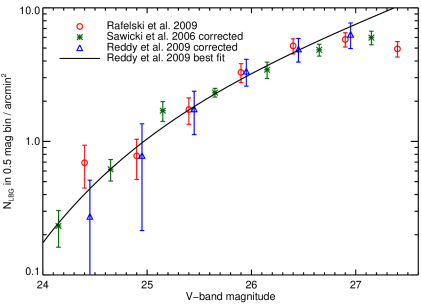
Figure 1.— Comparison of the number counts of $z\sim 3$ LBGs in 0.5 mag bins per square arcminute. The red circles are from Rafelski et al. (2009), the green crosses are from Sawicki & Thompson (2006) corrected for completeness, and the blue triangles are from Reddy & Steidel (2009) also corrected for completeness. The points from Reddy & Steidel (2009) are offset by 0.05 mag in order to avoid overlapping the Rafelski et al. (2009) points. The black line is the best-fit Schechter function (Schechter, 1976) from Reddy & Steidel (2009) with $\alpha=-1.73\pm 0.13$, $M^{*}_{\rm AB}(1700\AA)=-20.97\pm 0.14$, and $\phi^{*}=(1.71\pm 0.53$)$\times 10^{-3}$ Mpc^-3.

2. Observations

We implement our search for spatially extended star formation around $z\sim 3$ LBGs in the most sensitive high-resolution images available: the $V$ band image of the UDF taken with the Hubble Space Telescope (HST). This image is ideal because (1) of its high angular resolution (PSF FWHM = 0.^′′09), (2) at $z\sim 3$ the $V$ band fluxes correspond to rest-frame FUV fluxes, which are sensitive measures of SFRs, since short-lived massive stars produce the observed UV photons, and (3) the 1$\sigma$ point source limit of $V$=30.5 implies high sensitivity. Since most of the LBGs in the UDF are too faint for spectroscopic identification, the $u$ band is needed to find $z\sim 3$ LBGs via their flux decrement due to the Lyman limit through color selection and photometric redshifts. To this end, we acquired one of the most sensitive $u$ band images ever obtained and identified 407 LBGs at $z\sim 3$ (Rafelski et al., 2009, see also Nonino et al. (2009)).

Throughout the paper we utilize the $B$, $V$, $i^{\prime}$, and $z^{\prime}$ band (F435W, F606W, F775W, and F850LP, respectively) observations of the UDF (Beckwith et al., 2006), obtained with the Wide Field Camera on the HST Advanced Camera for surveys (ACS; Ford et al., 2002). These images cover 12.80 arcmin², although we only use the central 11.56 arcmin² which overlaps the $u$ band image from (Rafelski et al., 2009). The $u$ band image was obtained with the Keck I telescope and the blue channel of the Low-Resolution Imaging Spectrometer (LRIS; Oke et al., 1995; McCarthy et al., 1998) and has a 1$\sigma$ depth of 30.7 mag arcsec^-2 and a limiting magnitude of 27.6 mag. The sample described below also makes use of the observations taken with the NICMOS camera NIC3 in the $J$ and $H$ bands (F110W and F160W; Thompson et al., 2005) whenever the field of view (FOV) overlaps.

3. Sample Selection

In order to search for spatially extended star formation associated with $z\sim 3$ LBGs, we require a sample of such galaxies to form a super-stack of LBG images that we describe here. In Section 3.1, we compare the number counts of the $z\sim 3$ LBGs in the UDF to those in the literature. Then in Section 3.2, we select a subsample that is appropriate for stacking in order to improve the signal-to-noise (S/N) in the LBG outskirts as described in Section 4. Lastly, in Section 3.3 we investigate possible selection biases of the observations.

The samples in this paper are based on the $z\sim 3$ LBG sample of Rafelski et al. (2009), which contains 407 LBGs selected by using a combination of photometric redshifts and the $u$ band drop out technique (Steidel & Hamilton, 1992; Steidel et al., 1995, 1996a, 1996b). This selection of LBGs is enabled by the extremely deep $u$ band image described in Section 2, needed to reduce the traditional degeneracy of colors between $z\sim 3$ and $z\sim 0.2$ galaxies that can yield incorrect redshifts at $z\sim 3$ without the $u$ band (Ellis, 1997; Fernández-Soto et al., 1999; Benítez, 2000; Rafelski et al., 2009). Rafelski et al. (2009) found that the resultant sample is likely to have a contamination fraction of only $\sim 3\%$. Any such contamination will have a minimal effect on our results and is included in the uncertainties (see Section 4.3). In addition, Rafelski et al. (2009) found that the LBG sample is complete to $V\sim 27$ mag, limited by the depth of the $u$ band image.

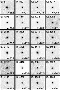
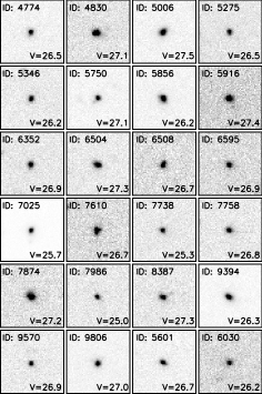
Figure 2.— Thumbnail images in the $V$ band of the 48 $z\sim 3$ LBG subsample. The thumbnails are 2.4 arcsec on a side, the same size as the composite image in Figure 3, which corresponds to $18.5$ kpc at $z\sim 3$.

3.1. Number Counts

In order to (1) be confident in our sample selection, (2) verify that we are probing the correct comoving volume, and (3) make completeness corrections in Sections 5 and 6 (as described in Appendix A), we compare the number counts of the $z\sim 3$ LBG selection from Rafelski et al. (2009) to the completeness corrected number counts from Sawicki & Thompson (2006) and Reddy & Steidel (2009) in Figure 1. The uncertainties shown from Rafelski et al. (2009) are only poisson and therefore have smaller error bars than those by Reddy & Steidel (2009). The points from Reddy & Steidel (2009) are offset by 0.05 mag for clarity, and their uncertainties include both poisson and field to field variations. The number counts and the best-fit Schechter function (Schechter, 1976) from Reddy & Steidel (2009) are converted to number of LBGs per half-magnitude bin using a similar conversion as in Reddy et al. (2008). Specifically, we use the $R$ band as a tracer of rest-frame 1700$\AA$ emission. The apparent measured $R$ magnitude, $R_{\rm AB}$, is converted from the absolute magnitude using the relation:

$$R_{\rm AB}=M_{\rm AB}(1700{\rm\AA})+5{\rm log}(d_{L}/10{\rm pc})+2.5{\rm log}(1+z)\;,$$ (1)

where $M_{\rm AB}(1700\AA)$ is the absolute magnitude at the rest-frame 1700$\AA$, and $d_{L}$ is the luminosity distance. We apply the $k$-correction from Rafelski et al. (2009) of $R_{\rm AB}-V_{\rm AB}$= $-$0.15 mag to get the $V$ band mag. We use a comoving volume of 26436 Mpc³ for the redshift interval 2.7$<z<$3.4 and an area of 11.56 arcmin² for the number count conversion. We adopt a Schechter function with parameters found by Reddy & Steidel (2009) of $\alpha=-1.73\pm 0.13$, $M^{*}_{\rm AB}(1700\AA)=-20.97\pm 0.14$, and $\phi^{*}=(1.71\pm 0.53$)$\times 10^{-3}$ Mpc^-3.

The resultant number counts agree nicely, and show that the completeness of the Rafelski et al. (2009) $z\sim 3$ LBG sample matches the previous completeness limit found of $V\sim 27$ magnitude. The agreement also suggests that the comoving volume for the redshift interval 2.7$<z<$3.4 is appropriate for the sample, which is important for the argument given in Section 5. More importantly, the agreement of the number counts allows us to use the best-fit Schechter function from Reddy & Steidel (2009) to determine the expected number of LBGs at fainter magnitudes, providing the needed information to make completeness corrections in Appendix A. We note that this luminosity function is valid to $R\sim 26.5$, after which the extrapolation to fainter magnitudes could be a potential source of error, and we address this below.

Table 1Properties of LBGs Included in Image Stack

ID	$z_{\rm phot}$	V	$u-V$	$B-V$	$V-z^{\prime}$	FWHM	Ellipticity
		(mag)	(mag)	(mag)	(mag)	(arcsec)
84	3.11${}_{-0.40}^{+0.40}$	26.56$\pm$0.02	2.40$\pm$0.35	0.70$\pm$0.05	0.03$\pm$0.04	0.24	0.18
862	3.18${}_{-0.41}^{+0.41}$	27.16$\pm$0.02	1.87$\pm$0.36	0.74$\pm$0.05	-0.44$\pm$0.05	0.12	0.14
906	2.68${}_{-0.36}^{+0.36}$	27.52$\pm$0.02	1.50$\pm$0.36	-0.10$\pm$0.04	-0.14$\pm$0.05	0.10	0.04
1217	2.75${}_{-0.37}^{+0.37}$	26.53$\pm$0.01	2.28$\pm$0.30	0.34$\pm$0.02	0.01$\pm$0.02	0.14	0.23
1273	3.03${}_{-0.39}^{+0.39}$	26.24$\pm$0.01	2.79$\pm$0.37	0.58$\pm$0.03	0.02$\pm$0.02	0.12	0.12
1414	2.86${}_{-0.38}^{+0.38}$	27.19$\pm$0.02	1.82$\pm$0.37	0.49$\pm$0.06	-0.03$\pm$0.05	0.10	0.13
1738	2.67${}_{-0.36}^{+0.36}$	26.27$\pm$0.01	1.05$\pm$0.08	0.03$\pm$0.02	-0.30$\pm$0.03	0.16	0.15
1753	3.44${}_{-0.43}^{+0.43}$	27.47$\pm$0.03	1.02$\pm$0.35	1.39$\pm$0.14	0.58$\pm$0.04	0.18	0.12
2581	3.40${}_{-0.43}^{+0.43}$	26.92$\pm$0.02	2.05$\pm$0.35	1.04$\pm$0.07	0.43$\pm$0.03	0.18	0.24
2595	2.97${}_{-0.39}^{+0.39}$	27.37$\pm$0.02	1.60$\pm$0.35	0.22$\pm$0.04	-0.17$\pm$0.05	0.13	0.05

Note. — $V$ magnitudes are total AB magnitudes, and colors are isophotal colors. $u$ band photometry is from Rafelski et al. (2009) and the rest are from Coe et al. (2006). Non-detections in the $u$ band are given 3$\sigma$ limiting magnitudes. This table is available in its entirety in a machine-readable form in the online journal. A portion is shown here for guidance regarding its form and content.

3.2. Catalogs of LBGs and Stars

We use two catalogs of $z\sim 3$ LBGs in this paper. The first is the full sample of 407 $z\sim 3$ LBGs as described in Rafelski et al. (2009). The sample redshift distribution is shown in Figure 12 of Rafelski et al. (2009) and has a mean photometric redshift of $3.0\pm 0.3$. The second (hereafter referred to as “subset sample”) is a sample of $z\sim 3$ LBGs selected to create a composite image to improve the signal-to-noise of the surface brightness profile described below. These LBGs are selected to be compact, symmetric, and isolated, similar to the selection done at higher redshift by Hathi et al. (2008). The LBGs are selected to be compact and symmetric to aid in stacking LBGs of similar morphology and physical characteristics such that the bright central regions of the LBGs overlap. They were also selected to be isolated from nearby neighbors to avoid coincidental object overlap and dynamically disturbed objects.

To select objects that are compact, symmetric, and isolated, we measure morphological parameters in the $V$ band image using $\tt SExtractor$ (Bertin & Arnouts, 1996). We experimented with different morphological parameters, such as asymmetry (Schade et al., 1995), concentration (Abraham et al., 1994, 1996), Gini coefficient (Lotz et al., 2004), and clumpiness (Conselice, 2003). However, we found that the best sample was selected based on the FWHM for compactness and ellipticity $\epsilon=(1-b/a)$ for symmetry, similar to the criteria in Hathi et al. (2008). Specifically, for the subset sample, we require that FWHM $\leq$ 0.^′′25 and $\epsilon\leq 0.25$, a slightly more conservative selection than Hathi et al. (2008). Lastly, to select isolated objects, we require that there are no other objects within 1.^′′4 brighter than 29th mag. These requirements yield a sample of 48 LBGs, representing $\sim 12\%$ of the $z\sim 3$ LBG sample, whose properties are compared in Section 3.3. We show this sample as thumbnails that are 2.4 arcsec on a side, which corresponds to 18.5 kpc at $z\sim 3$, in Figure 2, and a table with relevant information about the 48 LBGs in Table 1. Information on the full sample of 407 LBGs is available in Rafelski et al. (2009).

In addition to the two samples of LBGs, we also need a sample of stars for an accurate measurement of the point spread function (PSF) of the UDF images. We obtain this star sample from Pirzkal et al. (2005), using only those stars with confirmed grism spectra, which mostly consist of M dwarfs. We exclude the stars that are saturated, leaving 15 stars in the $V$ band image within our FOV with $V=25.7\pm 1.3$, more than adequate to measure the PSF. We note that a comparison of the star PSF with the LBGs shows that they are all resolved in the high resolution ACS images.

3.3. Comparison of the Subset and Full LBG Samples

We investigate whether the subset sample of 48 LBGs is drawn from the same parent population of the full sample of 407 LBGs by comparing the magnitude, color, and redshifts of two the samples. First, we find little variation in the magnitude distributions of the two samples, with a difference in the mean of $\sim 0.3$ mag. The subset sample is somewhat fainter, with the full sample having an average AB magnitude of $V=26.4\pm 0.9$ and the subset sample with $V=26.7\pm 0.6$. That is, there is a minor systematic selection of fainter LBGs in the subset sample, although this difference is not significant. The similar magnitude distribution of the rest-frame FUV flux suggests that the SFR of the two samples is similar.

Second, we compare the mean colors of the of the two samples and find the two samples have the same colors. We test this both for the distribution and for stacks of the LBGs. First, the mean of the distribution of the subset sample yields colors of $B-V$ = 0.5$\pm 0.4$, $V-i^{\prime}$ = 0.0$\pm 0.2$, and $i^{\prime}-z^{\prime}$ =0.0$\pm 0.1$, while the full sample has colors of $B-V$ = 0.6$\pm 0.4$, $V-i^{\prime}$ = 0.1$\pm 0.2$, and $i^{\prime}-z^{\prime}$ =0.0$\pm 0.1$. Second, the color of the stacked subset sample based on aperture photometry has colors of $B-V$ = 0.2$\pm 0.2$, $V-i^{\prime}$ = 0.1$\pm 0.2$, and $i^{\prime}-z^{\prime}$ =0.1$\pm 0.2$, while the full sample stack has colors of $B-V$ = 0.3$\pm 0.1$, $V-i^{\prime}$ = 0.1$\pm 0.1$, and $i^{\prime}-z^{\prime}$ =0.2$\pm 0.1$. These colors are not significantly different based on both the distribution and the stacked photometry uncertainties. The similar distribution of colors suggests that the two samples are made of the same stellar populations and that their star formation histories (SFHs) are similar.

Lastly, the two samples have very similar redshift distributions, with the same mean redshift of $3.0\pm 0.3$. We therefore conclude that the subset sample and full sample of LBGs are equivalent in magnitude, color, and redshift, and therefore are probably drawn from the same parent population of LBGs that have similar SFRs, stellar populations, and SFHs. Hence, we are relatively confident that the results determined below for the subset sample of LBGs are applicable to the full sample.

For the sake of completeness, we also consider stacking the full stack of LBGs in Appendix B. We note that stacking the full sample introduces contamination into the stack, such as nearby galaxies. In addition, bright parts of morphologically different galaxies contribute to the faint parts of other galaxies. We therefore do not use this as our primary stack, and take the full stack as an upper limit to the emission from the full sample of LBGs.

4. Analysis of UDF Images

The $V$ band image of the UDF is the most sensitive high resolution image covering the rest-frame FUV at $z\sim 3$ available. However, even this image does not reach the desired sensitivity to search for spatially extended star formation on scales up to $\sim$10 kpc (as shown below). We wish to increase the S/N high enough to probe down to low values of the SFR surface density ($\Sigma_{\rm SFR}$). Image stacking methods can be used to study the average properties of well defined samples in which individual objects do not have the necessary S/N (e.g., Pascarelle et al., 1996; Zibetti et al., 2004, 2005, 2007; Hathi et al., 2008).

We therefore create super-stacks of the LBG images in Section 4.1 and investigate how the sky-subtraction uncertainty affects those stacks in Section 4.2. Using the super-stack of the subset sample of LBGs described in Section 3.2, we determine the radial surface brightness profile of $z\sim 3$ LBGs in Section 4.3, which will be used for much of the analysis throughout the paper. Lastly, in Section 4.4, we investigate the effects of the Ly$\alpha$  line on the stacked image.

4.1. Image Stacks

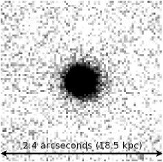
Figure 3.— Composite image in the $V$ band of the 48 $z\sim 3$ LBG subsample. Each stamp is 2.4 arcsec on a side, which corresponds to $18.5$ kpc at $z\sim 3$.

We create stacked composite images for the LBG subset sample, full LBG sample, and stars sample using custom IDL code. For each object, we fit a two-dimensional Gaussian using $\tt MPFIT$ (Markwardt, 2009) to determine a robust center. We then shift each object to be centered with sub-pixel resolution, interpolating with a damped sinc function. We then create thumbnail images for each object and combine all the objects by taking the median of all the thumbnails, yielding a robust stacked image which is not sensitive to outliers. While some of the individual thumbnails may have faint emission regions below the level of the isolation criteria, they do not contribute to the median because such emission would need to occur at the same pixels for a significant number objects to affect the median. Therefore, independent of the origin of any such faint regions, they do not affect their median, and therefore do not affect the final stack. While we are most interested in the $V$ band, we also carry out this procedure for the $B$, $V$, $i^{\prime}$, and $z^{\prime}$ bands and the stars sample. Figure 3 shows the stacked $V$ band image, as this corresponds to the rest-frame FUV luminosity at $z\sim 3$ which is a sensitive measure of the SFR. The image is 2.4 arcsec on a side, which corresponds to 18.5 kpc at $z\sim 3$.

We showed in Section 3.3 that the subset sample is representative of the full LBG sample and here investigate any possible variations in the radial surface brightness profile with magnitude and FWHM within the subsample itself. We check if these parameters affect the stack by creating three independent stacks of different brightnesses or FWHM. In the case of magnitude, we create one stack of the brightest 16 LBGs, a second stack of the next 16 LBGs, and a third stack with the faintest 16 LBGs, and repeat for FWHM. We find the profiles to be very similar and find that the magnitude and FWHM range does not affect our stack. We also investigate the change in the surface brightness profile color. We find that the variations of the LBG composite images for the $B$, $V$, $i^{\prime}$, and $z^{\prime}$ bands across radius are small compared to their uncertainties, and no clear change in color is obvious at any radius.

We also test the difference between taking the median and the mean of the images in our stack. The profiles of the mean stack are slightly higher at the bright end, but are very similar to the median stack starting at $\sim$0.^′′3. We chose to go with the median as it is more robust to possible contamination in the outskirts. In this way, we are not sensitive to contamination if it only occurs in a small subset of our sample.

In creating a stack of the star data to measure the PSF, we scale each star to the peak of the fitted two-dimensional Gaussian before stacking. For the PSF, we only care about the shape of the PSF, and not the actual value of the flux. Given the wide distribution of magnitudes of the stars, this scaling improves the PSF determination. We do not scale the LBGs before stacking, as we care about the actual measured flux in the outskirts of the LBGs. We find that scaling does not have a significant effect on the LBG stack due to the small range in brightnesses of the selected LBGs, with the radial surface brightness of the two stacks being consistent within the uncertainties, and this would therefore not alter our results.

4.2. Sky-subtraction Uncertainty

We hope to accurately characterize the sky background and the uncertainties due to the subtraction of this sky background. The sky-subtraction uncertainty of the UDF was carefully investigated by Hathi et al. (2008), and we follow their prescription for determining the $1\sigma$ sky-subtraction error. Hathi et al. (2008) found that it was more reliable to characterize the sky locally rather than globally for the entire image. For this reason, we redetermine the local sky background for the 407 $z\sim 3$ LBGs in our sample. First, we measure the sky background in each of the thumbnail images of the full LBG sample using IDL and the procedure $\tt MMM.pro$, adapted from the DAOPHOT routine by the same name (Stetson, 1987). This procedure iteratively determines the background, removing low probability outliers each time, until the sky background is determined. We then find the $1\sigma$ sky value by fitting a Gaussian to the distribution of sky values. For the $V$ band, this gives us a value for $\sigma_{\rm sky,ran}$ of $3.52\times 10^{-5}$ electrons s^-1, very similar to that found by Hathi et al. (2008) of $3.55\times 10^{-5}$ electrons s^-1. Using this number and the formalism in Hathi et al. (2008), we find a 1$\sigma$ sky-subtraction error of 30.01 mag arcsec^-2.

If the error is random, the uncertainty of the sky-subtraction will decrease as we stack more images together. In fact, for a median stack in the Poisson limit, the 1$\sigma$ uncertainty is $1.25/\sqrt{N}$, where $N$ is the number of images. We test this relation specifically for the UDF data as the error may not be completely random. We stack 48 blank thumbnails and compare the standard deviation of stacked pixels to the median of the standard deviations of each individual thumbnail and find the above relation holds to 99% accuracy. We are therefore confident that the sky-subtraction noise decreases with stacking as expected, yielding larger S/N values. For the stack of 48 LBGs from our subset sample, we find a 1$\sigma$ sky-subtraction error of 31.87 mag arcsec^-2. We use both of these sky-subtraction errors as our sky limits below in Section 4.3.

4.3. Radial Surface Brightness Profile

We extract a radial surface brightness profile from the super-stack of LBG images in Figure 4 using custom IDL code which yields identical results to the IRAF procedure $\tt ELLIPSE$. We use circular aperture rings with radial widths of 1.5 pixels in such a way that they do not overlap to avoid correlated data points while still finely probing the profile. We use custom code in order to facilitate using the bootstrap error analysis method to determine the uncertainties. Since we are stacking different objects with different characteristics, the uncertainty for the brighter regions will be dominated by the sample variance, and can be determined with the bootstrap method. Specifically, we bootstrap to get the uncertainty of the median of the LBGs by replacing a random fraction ($1/e\approx 37\%$) of the 48 LBG thumbnails with randomly duplicated thumbnails from the subset sample. We repeat this 1000 times to get a sample of composite images using the method described in Section 4.1, each with its own radial surface brightness profile. The resultant uncertainty is then the standard deviation of all the surface brightness magnitudes at each radius. This method is conservative, but includes all the uncertainties associated with the variance of the sample. Moreover, it helps takes into account possible errors introduced by possible contamination of our LBG sample by other objects, although as mentioned in Section 3, we believe this contamination fraction to be small.

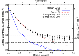
Figure 4.— Extracted surface brightness profile from the stacked image, where the black points are the 48 LBG composite profile and the blue line is the measured point-spread function from stars. The dotted red line is the best-fit Sérsic profile convolved with the PSF. The dashed line is the $1\sigma$ sky-subtraction error for one thumbnail image, while the dash-dotted line is the $1\sigma$ sky-subtraction error for the composite stack of 48 LBGs, as described in Section 4.2.

The solid blue line in Figure 4 represents the measured ACS $V$ band PSF determined from a stacked image of the 15 stars described in Section 3.2. The central surface brightness of the stars is scaled to match the LBGs. We note that the S/N of the star stack is higher than that of the LBG stack, even though it has a smaller number of objects in the stack, because the stars are brighter than the LBGs. Therefore the PSF is well determined, and we expect the uncertainties are dominated by the lower S/N LBG stack. The PSF declines more rapidly than the radial surface brightness profile at all radii, which shows that the LBGs are clearly resolved and that the median surface brightness profile of the LBGs is extended. The dashed line is the $1\sigma$ sky-subtraction error for one thumbnail image, while the dash-dotted line is the $1\sigma$ sky-subtraction error for the composite stack of 48 LBGs, as described in Section 4.2.

4.3.1 Sérsic Profile Fit

The dotted red line in Figure 4 shows the best fit Sérsic profile convolved with the ACS $V$ band PSF. We fit for the best Sérsic model to the composite LBG image by using the Levenberg–Marquardt least-squares minimization, with the $\chi^{2}$ calculated on a pixel by pixel basis for each possible model. The best fit values are $n=1.9\pm 0.04$ and $R_{e}=0.074\pm 0.001$ arcsec, where $n$ is the Sérsic index and $R_{e}$ is the effective radius, which includes half the light of the LBGs. We use the dimensionless scale factor $b$($n$) from Ciotti & Bertin (1999) such that $R_{e}$ is the half-light radius. The small $R_{e}$ value is likely due to our pre-selection of LBGs to be compact (see Section 3.2). While the fit has a good reduced chi-square $\chi^{2}/\nu$ of 1.27, it is not a very good fit to the data in the outer regions. The fit is dominated by the inner part of the profile with radii less than $\sim$0.^′′4, since the uncertainties are significantly smaller in that region. For radii larger than $\sim$0.^′′4, the profile deviates from the inner best-fit profile. This deviation is real, being above the PSF and the $1\sigma$ sky-subtraction error. This is similar to what Hathi et al. (2008) found when stacking LBGs at $z\sim 4--6$. The main constraint we have from this is that it suggests that the profile is similar to an exponential disk type profile. If we fit an exponential, it yields a worse fit with a $\chi^{2}/\nu$ of 1.4, and $R_{e}=0.068\pm 0.001$ arcsec. A bulge-disk model yields a slightly better fit in the outer regions, but does not improve the overall $\chi^{2}/\nu$. We note that we do not use the fit in the analysis below.

4.4. Effects of the Ly$\alpha$ Line on the Image Stack

We investigate possible contamination from Ly$\alpha$ emission on the image stack to ensure that the radial surface brightness profile is unaffected by Ly$\alpha$ emission from the LBGs. First, we note that Ly$\alpha$ only enters our $V$ band filter for about half our sample due to the redshift range sampled. Second, we find that due to the large width of the $V$ band filter, the Ly$\alpha$ line would have a very small effect. This is determined by taking the stacked LBG spectrum from Shapley et al. (2003), and comparing the flux in the $V$ band filter with and without the Ly$\alpha$ line. We find that the inclusion of the Ly$\alpha$ line yields an increase of 0.02 mag, a very small effect compared to our uncertainties. While our sample of LBGs is significantly fainter than the LBGs in the stacked spectrum from Shapley et al. (2003), we expect the average strength of the Ly$\alpha$ line to be similar due to the low escape fraction of ionizing radiation from LBGs (Shapley et al., 2006).

Moreover, we compare the radial surface brightness profile of the $V$ band stack and an equivalent stack in the $i^{\prime}$ band. The Ly$\alpha$ line does not enter the $i^{\prime}$ band filter throughout our redshift range, making the $i^{\prime}$ band an excellent test to check if the radial surface brightness profile is affected by the Ly$\alpha$ line. We find that the $V$ and $i^{\prime}$ bands have the same radial surface brightness profile within their uncertainties, with no systematic shifts. This suggests that the Ly$\alpha$ line has little to no effect, even if the Ly$\alpha$ line were more extended than the continuum.

5. Direct Inferences from the Data

The surface brightness profile of the stacked image indicates the presence of spatially extended star formation around LBGs. In this section, we describe how to connect this emission, which corresponds to the rest-frame FUV radiation intensity, to the SFR surface density. We then compare the covering fraction of this emission to that of the gas responsible for the star formation in Section 5.2. Specifically, in order to determine what types of gas can be responsible for the observed emission, we compare its covering fraction to that of atomic-dominated gas in Section 5.2.1 and to that of molecular-dominated gas in Section 5.2.2. Then in Section 5.3 and 5.4, we calculate the in situ SFR, $\dot{\rho_{*}}$, and metal production based on the integrated flux measured in the outskirts of LBGs.

5.1. Connecting the Observed Intensity to the SFR Surface Density

In order to investigate how the measured star formation relates to the underlying gas, we require a relation between star formation and gas properties. Star formation occurs in the presence of cold atomic and/or molecular gas, according to the KS relation given by

$$\Sigma_{\rm SFR}=K\times\left(\frac{\Sigma_{\rm gas}}{\Sigma_{\rm c}}\right)^{\beta}\;.$$ (2)

This relation holds for nearby disk galaxies in which $\Sigma_{\rm gas}$ is the mass surface density perpendicular to the plane of the disk, $\Sigma_{\rm c}=1$$M_{\odot}$pc^-2, $K=K_{\rm Kenn}$=(2.5$\pm$0.5)$\times$10^-4 $M_{\odot}{\rm\ yr^{-1}\ kpc^{-2}}$, and ${\beta}$=1.4$\pm$0.15 (Kennicutt, 1998a, b). There has been much recent work on improving both our understanding of this relation, and measuring the values of $K$ and $\beta$ (e.g., Leroy et al., 2008; Bigiel et al., 2008; Krumholz et al., 2009b; Gnedin & Kravtsov, 2010; Genzel et al., 2010; Bigiel et al., 2010b). When only considering molecular gas, the relationship has a flatter slope of ${\beta}$=0.96$\pm$0.07 (Bigiel et al., 2008) or ${\beta}\sim 1.1$ (Wong & Blitz, 2002). We use the original values from (Kennicutt, 1998a) when considering the total gas density to simplify comparisons with other work, and ${\beta}$=1.0 and $K$=$K_{\rm Biegel}$=(8.7$\pm$1.5)$\times$10^-4 $M_{\odot}{\rm\ yr^{-1}\ kpc^{-2}}$ when considering only molecular gas. We note that the $K$ value given here used for molecular gas is modified from Bigiel et al. (2008) to use the same $\Sigma_{\rm c}=1~{}$$M_{\odot}$pc^-2 value as above.

Rewriting the KS relation in terms of the column density of the gas, we get

$$\Sigma_{\rm SFR}=K\times\left(\frac{N}{N_{c}}\right)^{\beta},$$ (3)

where the scale factor $N_{c}$=1.25$\times$10²⁰ cm^-2 (Kennicutt, 1998a, b) and $N$ is the hydrogen column density. We note that this is only valid above the critical column density, which is usually associated with the threshold condition for Toomre instability. For H I gas in local galaxies, it is observed to range between 5$\times$10²⁰ cm^-2 and 2$\times$10²¹ cm^-2 (Kennicutt, 1998b).

In order to connect $\Sigma_{\rm SFR}$ to the observations, we require a relation between observed intensity, corresponding to rest-frame FUV emission, and observed column density, $N$. Following Wolfe & Chen (2006, equation (3)), we find that for a fixed value of $N$, the intensity averaged over all disk inclination angles is given by

$$\langle I_{\nu_{0}}^{\rm obs}\rangle=\frac{C\Sigma_{\rm SFR}}{4{\pi}(1+z)^{3}{\beta}}\;,$$ (4)

where $z$ is the redshift, and $C$ is the conversion factor from SFR to FUV ($\lambda\sim 1500\AA$) radiation, with $C=8.4\times 10^{-16}$ erg cm^-2 s^-1 Hz^-1($M_{\odot}{\rm\ yr^{-1}\ kpc^{-2}}$)^-1 (Madau et al., 1998; Kennicutt, 1998b). We use the same value of $C$ as Wolfe & Chen (2006) corresponding to a Salpeter IMF. The result in Equation (4) assumes that the star formation occurs in disks inclined on the plane of the sky by randomly selected inclination angles and averages over all possible angles (see Wolfe & Chen, 2006).

5.2. Covering Fraction of LBGs Compared to the Underlying Gas

The covering fraction of observed star formation should be consistent with that of its underlying gas. We therefore investigate whether the covering fraction of the outer parts of LBGs is consistent with the covering fraction of atomic-dominated gas in Section 5.2.1 and molecular-dominated gas in Section 5.2.2. This consistency check yields insights into the nature of the observed star formation and validates the hypothesis that the outskirts of LBGs consist of atomic-dominated gas, which is used in subsequent sections of the paper.

We calculate the cumulative covering fraction, $C_{A}$, for gas columns greater than some column density, $N$, by integrating the H column-density distribution function $f(N_{\rm H},X)$, where H is either H Ior H₂. Specifically,

$$C_{A}(N)={\int_{X_{\rm min}}^{X_{\rm max}}}dX{\int_{N}^{N_{\rm max}}dN_{\rm H}f(N_{\rm H},X)}\;,$$ (5)

where $f(N_{\rm H},X)$ is the observed column-density distribution function of the hydrogen gas, $N_{\rm max}$ is the maximum column-density considered, and $X$ is the absorption distance with $dX$ being defined as

$$dX\equiv\frac{H_{0}}{H(z)}(1+z)^{2}dz\;,$$ (6)

where $H_{0}$ is the Hubble constant and $H(z)$ is the Hubble parameter at redshift $z$. For $X_{\rm min}$ and $X_{\rm max}$ we use the same redshift interval as in Section 3.1, namely $2.7<z<3.4$ corresponding to $6.6<X<9.2$. The covering fraction depends strongly on the column-density distribution function, which is different for atomic and molecular gas. Below we investigate the covering fraction for both cases.

5.2.1 Covering Fraction of Atomic-dominated Gas

There is strong evidence to support the association of LBGs and neutral atomic-dominated H I gas, i.e., DLAs (see Section 1), and we therefore investigate whether the covering fraction of the outer parts of LBGs is consistent with the covering fraction of DLAs. If the outer regions of LBGs truly consist of DLA gas, then the covering fractions as functions of the surface brightnesses should be consistent. In this subsection, we work under the hypothesis that the observed FUV emission in the outskirts of LBGs is from in situ star formation in atomic-dominated gas and compare the observed covering fraction to that of the gas distribution.

In order to calculate the covering fraction using Equation (5), we require $f(N_{\rm H},X)$ for atomic-dominated gas. The observed H I column-density distribution function, $f(N_{{\rm HI}},X)$, is obtained by a double power-law fit to the Sloan Digital Sky Survey data:

$$f(N_{{\rm HI}},X)=k_{3}\left(\frac{N}{N_{0}}\right)^{\alpha}\;,$$ (7)

where $k_{3}$=(1.12$\pm$0.05)$\times$10^-24 cm², $\alpha$=$\alpha_{3}$=$-$2.00$\pm$0.05 for $N\leq N_{0}$ and $\alpha$=$\alpha_{4}$=$-$3.0 for $N>N_{0}$, where $N_{0}=3.54^{+0.34}_{-0.24}\times 10^{21}$ cm^-2 (Prochaska et al., 2005; Prochaska & Wolfe, 2009). The value of $\alpha_{4}$ used is different than measured in (Prochaska & Wolfe, 2009), to remain consistent with our formulation of randomly oriented disks in Section 6, and is predicted to be $-3.0$, and we use this value for the covering fraction to be consistent. Although this value of $\alpha_{4}$ is different than the value in Prochaska & Wolfe (2009), the uncertainties are quite large due to low numbers of very high column density DLAs, and it is quite similar to the value found by Noterdaeme et al. (2009) of $\alpha_{4}$=$-$3.48.

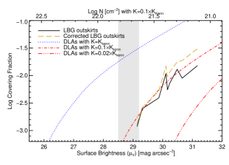
Figure 5.— Cumulative covering fraction of DLA systems with columns greater than some column density $N$ (and therefore surface brightness), compared to the covering fraction of the observed $z\sim 3$ LBG outskirts greater than some surface brightness. The blue dotted line is the DLA covering fraction for DLAs with $K=K_{\rm Kenn}$, the red dash-dotted line is for $K=0.1\times K_{\rm Kenn}$, and the red triple-dot-dashed line is for $K=0.02\times K_{\rm Kenn}$. The solid black line is the covering fraction for the LBG outskirts, while the gold long-dashed line is the same corrected for completeness. The gray filled region represents the transition region mentioned in Section 5.2.2. The top $x$-axis coordinates are the column densities corresponding to the surface brightnesses using an efficiency of $K=0.1\times K_{\rm Kenn}$.

We note that Noterdaeme et al. (2009) find slightly different values for $k_{3}$ and $\alpha_{3}$ than Prochaska & Wolfe (2009), with $k_{3}$=8.1$\times$10^-24 cm² and $\alpha$=$\alpha_{3}$=$-$1.60 for $N\leq N_{0}$, corresponding to a flatter slope. We use the values from Prochaska & Wolfe (2009) and describe how the differing values affect our results below. Also, although the normalization of $f(N_{{\rm HI}},X)$ varies with redshift, the variations for our redshift interval are not large and do not strongly affect $C_{A}$. Using the Prochaska & Wolfe (2009) values for $f(N_{{\rm HI}},X)$, and $N_{\rm max}=10^{22}$ cm^-2, we calculate the covering fraction using Equation (5) and the corresponding expected $\mu_{V}$ from Equations (3) and (4), where $\mu_{V}=-2.5{\rm log}\langle I_{\nu_{0}}^{\rm obs}\rangle-Z$, and $Z$ is the AB magnitude zero point of 26.486.

We compare the cumulative covering fraction of DLAs to the observed covering fraction of the outer regions of the LBGs in Figure 5. The blue dotted line is the DLA covering fraction for DLAs forming stars according to the KS relation, with $K=K_{\rm Kenn}$. The red lines are for less efficient star formation where the dash-dotted line represents $K=0.1\times K_{\rm Kenn}$ and the triple-dott-dashed line represents $K=0.02\times K_{\rm Kenn}$. The black line is the covering fraction for the observed emission in the outskirts of LBGs in the UDF, which is just the area covered by the outskirts of LBGs up to $\mu_{V}$ divided by the total area probed, 11.56 arcmin². The covered area is obtained from the radial surface brightness profile and the 407 observed LBGs in this area. The observed covering fraction depends on the depth of the images and therefore requires a completeness correction for faint objects that are missed: we discuss this completeness correction in Appendix A. The completeness corrected covering fraction for LBGs is the dashed gold long-dashed line, and is the curve that we compare to the DLA lines below. We ignore the data at a radius $>0.8$ arcsec ($\sim 6$kpc) to only include data with S/N$>$3, however, we expect a continuation of the observed trends. We note that we are only sampling the top end of the DLA distribution function, and therefore the covering fraction shown is a small fraction (about a tenth) of the total covering fraction of DLAs. When considering all DLAs, we cover about one-third of the sky, i.e., ${\rm log}(C_{A})\sim-0.5$. We note that if we use the Noterdaeme et al. (2009) values for $f(N_{{\rm HI}},X)$, then the DLA lines move up and to the left (i.e., cover more of the sky).

Under the hypothesis that the outskirts of LBGs are comprised of atomic-dominated gas (i.e., DLAs) which is responsible for the observed emission, then we expect the covering fraction of the DLA gas to be equal to the covering fraction of the outskirts of LBGs. The blue dotted line for DLAs following the KS relation would therefore only be consistent with the covering fraction of the outskirts of LBGs if much of the DLA gas is not surrounding LBGs. This possibility was constrained by (Wolfe & Chen, 2006), who found that DLAs would need to be forming at significantly lower SFR efficiencies if this was the case. On the other hand, we find that the covering fraction of the outskirts of LBGs is consistent with DLAs having SFR efficiencies of $K\gtrsim 0.1\times K_{\rm Kenn}$, at which point the covering fraction is roughly equal. This covering-factor analysis provides evidence that if the outskirts of LBGs are comprised of DLA gas, then the SFR efficiency of this atomic-dominated gas at $z\sim 3$ is about 10% of the efficiency for local galaxies.

Moreover, the cumulative covering fraction shows that there is sufficient DLA gas available to be responsible for the emission in the outskirts of LBGs for SFR efficiencies $\gtrsim 10$%. We investigate this lower SFR efficiency further in Section 6, where we find an efficiency closer to 5%, which is only a factor of $\sim$2 different than the efficiency determined from the covering fraction. We note that systematic uncertainties due to assumptions throughout both quantities could easily be off by a factor of two, and so the general agreement of the covering fraction at low SFR efficiencies is reassuring, and we are not concerned about the minor disagreement.

5.2.2 Covering Fraction of Molecular Gas

In the previous subsection, we worked under the hypothesis that the observed FUV emission in the outskirts of LBGs is from in situ star formation in atomic-dominated gas. However, it is possible that this star formation occurs in molecular-dominated gas. We consider this scenario here, and compare the covering fraction of molecular-dominated gas, where the majority of the hydrogen gas is molecular, to our observations.

In order to calculate the covering fraction using Equation (5), we require $f(N_{\rm H},X)$ for molecular-dominated gas. We use the observed molecular column-density distribution function, $f(N_{\rm H_{2}})$, from Zwaan & Prochaska (2006), who obtained a lognormal fit to the BIMA SONG data (Helfer et al., 2003),

$$f(N_{\rm H_{2}})=f^{*}~{}{\rm exp}\left[\left(\frac{{\rm log}N-\mu}{\sigma}\right)^{2}/~{}2\right]\;,$$ (8)

where $\mu=20.6$, $\sigma=0.65$, and the normalization $f^{*}$ is $1.1\times 10^{-25}$ cm² (Zwaan & Prochaska, 2006). We use the molecular version of the KS relation discussed in Section 5, where ${\beta}$=1.0 and $K$=$K_{\rm Biegel}$=8.7$\times$10^-4 $M_{\odot}{\rm\ yr^{-1}\ kpc^{-2}}$, and we let $N_{\rm max}=10^{24}$ cm^-2, the largest observed value for the $f(N_{\rm H_{2}})$ function used (Zwaan & Prochaska, 2006). However, $f(N_{\rm H_{2}})$ is not observationally determined at $z\sim 3$, and likely evolves over time, and we investigate such a possibility below.

The evolution of $f(N_{\rm H_{2}})$ would either be due to a change in the normalization or a change in the shape. The shape of the atomic gas column-density distribution function, $f(N_{\rm H_{I}})$, has not evolved between $z=0$ and $z=3$ (Zwaan et al., 2005; Prochaska et al., 2005; Prochaska & Wolfe, 2009), but the normalization has increased by a factor of two. In the case of H₂, we consider the instance in which only the normalization ($f^{*}$) evolves, then we are looking for a change in $\Omega_{\rm H_{2}}$ at $z=0$ to $\Omega_{\rm H_{2}}$ at $z=3$. While theoretical models predict that $\Omega_{\rm H_{2}}(z=3)/\Omega_{\rm H_{2}}(z=0)$ is $\sim 4$, their similar prediction for atomic gas does not match observations (Obreschkow & Rawlings, 2009). Alternatively, we can determine an upper limit of the evolution of $f^{*}$ using the evolution of $\dot{\rho_{*}}$ for galaxies between $z=0$ and $z=3$, assuming that the evolution in $f(N_{\rm H_{2}})$ is only due to the normalization, and there is no evolution in the KS law for molecular gas between $z=0$ and $z=3$ (Bouché et al., 2007; Daddi et al., 2010; Genzel et al., 2010, see Section 6.3). Specifically, studies have found that $\dot{\rho_{*}}$$(z=3)$/$\dot{\rho_{*}}$$(z=0)\sim 10$ (Schiminovich et al., 2005; Reddy et al., 2008), and therefore $f^{*}$ changes at most by a factor of 10, if we assume that the contribution from atomic gas is small. This is used as an upper limit to the evolution of $f^{*}$, and we are not suggesting that this is the correct evolution.

We plot the covering fractions of molecular gas at $z=3$ in Figure 6. We consider three cases for $f(N_{\rm H_{2}})$: (1) no evolution as a purple short-dashed line, (2) evolution with a factor of four increase in $f^{*}$ based on the model by Obreschkow & Rawlings (2009) as a pink triple-dashed line, and (3) evolution with a factor of 10 increase in $f^{*}$ based on the observed evolution in $\dot{\rho_{*}}$ as a cyan dot-dashed line. The gray lines continuing these three lines are extrapolations of the data to lower column densities than observed. We note that the column densities on the top $x$-axis of the plot now are for $K=K_{\rm Biegel}$.

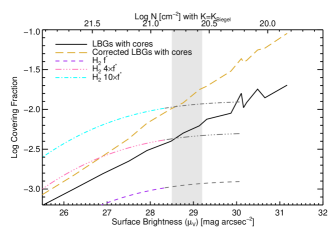
Figure 6.— Cumulative covering fraction of gas with columns greater than some column density $N$ (and therefore surface brightness). This figure is similar to Figure 5, but makes comparisons to the covering fractions of molecular gas rather than atomic-dominated gas. The solid black line is the covering fraction for LBGs starting from the center of the LBG core, and the gold long-dashed line is the same corrected for completeness. The purple short-dashed line is the covering fraction of molecular hydrogen with no evolution at $z\sim 3$, the pink triple dot-dashed line is the same with an evolution of four times $f^{*}$ (the normalization of the column-density distribution function of molecular gas) and the cyan dot-dashed line is the same with an evolution of 10 times $f^{*}$. The gray lines continuing the purple, pink, and cyan lines are extrapolations of the data to lower column densities. The gray filled region represents the transition region mentioned in Section 5.2.2. The top $x$-axis coordinates are the column densities corresponding to the surface brightnesses using an efficiency of $K=K_{\rm Biegel}$ and $\beta=1$, valid for molecular gas.

These covering fractions of molecular gas are compared to the LBG profile including the inner cores in Figure 6. The LBG covering fraction is now modified to include the LBG cores which are composed of molecular-dominated gas, and the new LBG covering fraction is plotted as a solid brown line. We again ignore the data at a radius $>0.8$ arcsec ($\sim 6$kpc) to only include data with S/N$>$3. This covering fraction is also corrected for completeness similar to Section 5.2.1, except this time we include the cores of the LBGs and make no distinction between the outskirts and the inner parts of the LBGs, and is described in Appendix A.1. We plot this corrected covering fraction as a gold long-dashed line. This correction is quite large, as even though the cores cover a smaller area than the outskirts, the cores of fainter missed LBGs contribute at every surface brightness as we go fainter. Since there are significantly more faint LBGs than bright LBGs, there are significantly more LBG cores contributing to each surface brightness than there are LBGs with outskirts at those same surface brightnesses. This correction assumes that all the star formation comes from molecular-dominated gas, and therefore all the cores of fainter LBGs are included.

As in Section 5.2.1, we expect the covering fraction of the gas to be equal to the covering fraction of the LBGs forming out of that gas. In the case of purely molecular gas, the upper limit of the covering fraction ($10\times f^{*}$) of the gas is only consistent to $\mu_{V}\sim 28.5$. At $\mu_{V}\gtrsim 28.5$, the covering fraction of LBGs is larger than that of the molecular gas. In order to have a covering fraction larger than all the corrected LBG emission, we would require an evolution of $f^{*}$ by a factor of more than 60, which is not very likely.

We have just shown that the predicted covering factor for molecules is inconsistent with our results for $\mu_{V}\gtrsim 28.5$. At the same time, our results for atomic-dominated hydrogen do not apply for $\mu_{V}$ brighter than $\sim 29$, due to the atomic-dominated H I gas cutoff of $N_{\rm HI}\leq 10^{22}$cm^-2. Therefore, the surface brightness interval from 28.5 $\lesssim\mu_{V}\lesssim$ 29.2 is not simultaneously consistent with the neutral atomic-dominated gas nor the molecular gas’ covering fractions. This lower bound on $\mu_{V}$ is based on comparing the LBG data compared to 10 times $f^{*}$, and for lower evolutions of $f^{*}$, this begins at even brighter $\mu_{V}$. This result is reasonable if the LBG outskirts consist of atomic-dominated gas. In this scenario, there would need to be a transition region between atomic-dominated and molecular-dominated gas, where star formation occurs in both phases. We note that in this hybrid region, the corrected covering fraction of LBGs is not correct, as we would be adding the star formation in the cores of missed LBGs to the outskirts presumably composed of atomic-dominated gas. The true correction would lie somewhere between the black solid line and the gold long-dashed line. We take the molecular gas covering fraction results as evidence that the outskirts of LBGs consist of atomic-dominated gas, which is consistent with our underlying hypothesis for this paper.

Table 2SFR, $\dot{\rho_{*}}$, and Metallicity

$\theta_{\rm low}$	$\theta_{\rm high}$	$R/H$	$\rm SFR$	$\dot{\rho_{*}}$	$\dot{\rho_{*}}$ Corrected	$f$	$Z$	$\rm[M/H]$
(arcsec)	(arcsec)		($M_{\odot}$ yr-1)	($M_{\odot}$ yr-1 Mpc-3)	($M_{\odot}$ yr-1 Mpc-3)		$(Z_{\odot}$)
0.405	0.765	10	$0.118\pm 0.002$	$(1.82\pm 0.03)\times 10^{-3}$	$(3.75\pm 0.03)\times 10^{-3}$	$0.084\pm 0.001$	$0.12\pm 0.05$	$-0.9\pm 0.4$
0.405	0.765	100	$0.059\pm 0.001$	$(0.91\pm 0.01)\times 10^{-3}$	$(1.87\pm 0.01)\times 10^{-3}$	$0.084\pm 0.001$	$0.12\pm 0.05$	$-0.9\pm 0.4$
0.405	1.125	10	$0.187\pm 0.005$	$(2.87\pm 0.08)\times 10^{-3}$	$(5.91\pm 0.08)\times 10^{-3}$	$0.126\pm 0.002$	$0.19\pm 0.07$	$-0.7\pm 0.4$
0.405	1.125	100	$0.093\pm 0.002$	$(1.44\pm 0.04)\times 10^{-3}$	$(2.95\pm 0.04)\times 10^{-3}$	$0.126\pm 0.002$	$0.19\pm 0.07$	$-0.7\pm 0.4$

Note. — The integrated SFR and $\dot{\rho_{*}}$ in the outskirts of LBGs. We integrate from the point where the theoretical models for DLA gas and the LBG data overlap, in order to probe the hypothesis that the FUV emission in this region is from in situ star formation in DLA gas associated with the LBGs.

5.3. Measurements of the SFR and $\dot{\rho_{*}}$ in the Outskirts of LBGs

In addition to calculating the efficiency of the SFR, we can also calculate the mean SFR, $\langle{\rm SFR}\rangle$, and $\dot{\rho_{*}}$ in the outskirts of LBGs by integrating the rest-frame FUV emission in the outer areas. These measurements allow us to calculate the metals produced in the outskirts of LBGs in Section 5.4 and to put a limit on the total $\dot{\rho_{*}}$ contributed by DLA gas. Similar to Wolfe & Chen (2006), we assume that DLAs are disk like structures, or any other type of gaseous configurations with preferred planes of symmetry. We note that while we work this out for DLA gas, the only assumption in our derivation is that the outskirts have preferred planes of symmetry such, as disks. Even if the outskirts of LBGs are not DLA gas, such an assumption is still valid given the rotation curves measured for high redshift LBGs (e.g., Schreiber et al., 2009) and the predictions by simulations (Brooks et al., 2009; Ceverino et al., 2010).

For these calculations, we need $\Sigma_{\nu}^{\perp}$, the luminosity per unit frequency interval per unit area projected perpendicular to the plane of the disk. Specifically, we solve for $\Sigma_{\nu}^{\perp}$ as a function of $\langle I_{\nu_{0}}^{\rm obs}\rangle$ averaged over all inclination angles. We find that

$$\Sigma_{\nu}^{\perp}\equiv\frac{4\pi(1+z)^{3}\langle I_{\nu_{0}}^{\rm obs}\rangle}{\ln(R/H)}\;,$$ (9)

where $R$ is the radius and $H$ is the scale height of the model disks, which holds in the limit $R\gg H$. We calculate $\Sigma_{\nu}^{\perp}$ for a range in aspect ratios, with $R/H$ values from 10 to 100, covering a range from thick disks, as possibly seen at high redshift (e.g., Schreiber et al., 2009), all the way to thin disks resembling the Milky Way. We then calculate the mean SFR by integrating $\Sigma_{\nu}^{\perp}$ across the outer region of the LBG stack, and find that

$$\langle{\rm SFR}\rangle=\frac{8\pi(1+z)^{3}}{C^{\prime}{\rm ln}(R/H)}\int_{\theta_{\rm low}}^{\theta_{\rm high}}2\pi{d_{A}}^{2}\langle I_{\nu_{0}}^{\rm obs}(\theta)\rangle\theta d\theta\;,$$ (10)

where $d_{A}$ is the angular diameter distance, $\theta$ is the radius in arcseconds, $\theta_{\rm low}$ is the minimum radius for the outer region, and $\theta_{\rm high}$ is the maximum radius. $I_{\nu_{0}}^{\rm obs}(\theta)$ comes from the radial surface brightness profile from Section 4.3 and depends on $\mu_{V}(\theta)$, namely $I_{\nu_{0}}^{\rm obs}(\theta)=10^{-0.4(\mu_{V}(\theta)+48.6)}$. The SFR depends on the inclination angles of the disks for a given $I_{\nu_{0}}^{\rm obs}$ and includes a factor of two for averaging over all inclination angles.

In order to find the $\langle{\rm SFR}\rangle$ in the outer regions of LBGs, we need to designate a radius at which to start integrating the LBG stack, and a comparison of the theoretical model to the data in Section 6.2 yields this radius. The $\langle{\rm SFR}\rangle$ is independent of the theoretical framework developed later in Section 6 and does not depend on the efficiency of the gas. It is purely a measurement of the star formation occurring in the gas. However, it requires a minimum radius to define the beginning of the outer region of the LBGs. Specifically, we pick the smallest radius that corresponds to the first point in Figure 9 where we demonstrate that the smallest radius of atomic-dominated gas corresponds to 0.^′′4. We note that when we refer to spatially extended emission star formation throughout the paper, we are referring to emission at radii larger than 0.^′′4. We also require a second point that we integrate out to, for which we use two different values. First, we use the radius of 0.^′′8, which corresponds to the largest radius above 3$\sigma$. Second, we integrate to 1.^′′1 , corresponding to the furthest point for which we measured $\mu_{V}$ in Figure 4. Table 2 lists the SFRs for different combinations of $R/H$ and $\theta_{\rm high}$. Since we integrate over the radii where the LBG data intersect the theoretical models for the DLA gas, the FUV emission from this region may be from the in situ star formation in DLA gas associated with the LBGs (see Section 7).

After we have the SFR we can calculate values for the SFR per unit comoving volume, $\dot{\rho_{*}}$, via $\dot{\rho_{*}}$=SFR$\times N_{\rm LBG}/V_{\rm UDF}$, and they are tabulated in Table 2. However, since $\dot{\rho_{*}}$ depends on $N_{\rm LBG}$, we perform a completeness correction as described in Appendix A.2. The resultant completeness corrected $\dot{\rho_{*}}$ are listed in Table 2. While there is a range in the acceptable values for both the SFR and $\dot{\rho_{*}}$, we find that the extended emission has $\langle{\rm SFR}\rangle$ $\sim 0.1$ $M_{\odot}$ yr^-1 and $\dot{\rho_{*}}$ $\sim 3\times 10^{-3}$ $M_{\odot}$ yr^-1 Mpc^-3.

We take this measured $\dot{\rho_{*}}$ in conjunction with the upper limit found in Wolfe & Chen (2006) to calculate the total $\dot{\rho_{*}}$ from neutral atomic-dominated gas at $z\sim 3$. Specifically, Wolfe & Chen (2006) constrain $\dot{\rho_{*}}$ for regions in the UDF without LBGs, which complements the results from this study for regions containing such objects. Together, we constrain all possibilities for the star formation from such gas. Wolfe & Chen (2006) place a conservative upper limit on $\dot{\rho_{*}}$ contributed by DLAs with column densities greater than $N_{\rm min}=2\times 10^{20}$cm^-2, finding $\dot{\rho_{*}}$ $<$ $4.0\times 10^{-3}$ $M_{\odot}$ yr^-1 Mpc^-3. Combining this with our largest possible value of the completeness corrected $\dot{\rho_{*}}$ in Table 2 of $\dot{\rho_{*}}$=$5.91\times 10^{-3}$ $M_{\odot}$ yr^-1 Mpc^-3, we calculate an upper limit on the total $\dot{\rho_{*}}$ contributed by DLA gas. We find a conservative upper limit of $\dot{\rho_{*}}$$<$ $9.9\times 10^{-3}$ $M_{\odot}$ yr^-1 Mpc^-3, corresponding to $\sim 10\%$ of the $\dot{\rho_{*}}$ measured in the inner regions of LBGs at $z\sim 3$ (Reddy et al., 2008).

5.4. Metal Production in the Outskirts of LBGs

Under the hypothesis that the outskirts of LBGs are composed of atomic-dominated gas, we can calculate the metals produced due to in situ star formation from $z=10$ to $z=3$, and compare this to the metals observed in DLAs at $z=3$. The metal production can be measured from the outskirts of the LBG composite since the FUV luminosity is a sensitive measure of star formation, since the massive stars produce the UV photons as well as the majority of the metals. The comoving density of metals produced is obtained by integrating the comoving SFR density ($\dot{\rho_{*}}$) from the most recent galaxy surveys (Bouwens et al., 2010a, b; Reddy & Steidel, 2009). We note that the resultant metallicities are only valid if the outskirts of LBGs are composed of atomic-dominated gas, as we divide by the H I mass density, $\rho_{\rm HI}$, to obtain the metallicity.

First, we integrate $\dot{\rho_{*}}$ for all LBGs from $z\sim 3$ to $z\sim 10$ using the $\dot{\rho_{*}}$ values from Bouwens et al. (2010a, b) and Reddy & Steidel (2009) to calculate the total mass of metals produced in LBGs by $z\sim 3$ similar to Pettini (1999, 2004, 2006) and Wolfe et al. (2003a). Specifically, we calculate the comoving mass density of stars at $z\sim 3$ by

$$\rho_{*,{\rm LBG}}=\int^{z=10}_{z=3}\dot{\rho}_{*,{\rm LBG}}\frac{dt}{dz}dz=1.1\times 10^{8}~{}M_{\odot}~{}{\rm Mpc^{-3}}$$ (11)

where

$$\frac{dt}{dz}=\frac{1}{(1+z)H(z)}\;.$$ (12)

In order to obtain the comoving mass density of stars in the outskirts of LBGs, we multiply this result by the fraction of $\dot{\rho_{*}}$ observed in the outer region of the composite LBG stack compared to the total $\dot{\rho_{*}}$ observed, $f$, which we list in Table 2. We can then calculate the total mass in metals produced by $z\sim 3$ using the estimated conversion factor $\dot{\rho}_{\rm metals}=(1/64)~{}\dot{\rho_{*}}$ by Conti et al. (2003), which is a factor of 1.5 lower than the metal production rate originally estimated by Madau et al. (1996). The metallicity of the presumed DLA gas is then calculated by dividing by $\rho_{\rm HI}$ at $z\sim 3$, where we use average value of $\rho_{\rm HI}$ over the redshift range $2.4\lesssim z\lesssim 3.5$ of $(9.0\pm 0.1)\times 10^{7}$ $M_{\odot}$ Mpc^-3 (Prochaska & Wolfe, 2009). The final metallicities are tabulated in Table 2 in terms of the solar metallicity, where $Z_{\odot}$ = 0.0134 (Asplund et al., 2009; Grevesse et al., 2010). The metallicities range from $0.12Z_{\odot}$ to $0.19Z_{\odot}$, similar to DLA metallicities (see Section 7.6). We note that $f$ is independent of the disk aspect ratio ($R/H$), and therefore so is the metallicity.

6. Star Formation Rate Efficiency in Neutral Atomic-dominated Gas

In our search for spatially extended LSB emission around LBGs, we aim to further our understanding of the connection between the DLA gas studied in absorption and the star formation needed to explain the characteristics of the DLA gas. Specifically, Wolfe & Chen (2006) searched for isolated LSB emission of DLAs, away from known LBGs, in the UDF and found conservative upper limits on the SFR per unit comoving volume, $\dot{\rho_{*}}$. These limits constrain the in situ SFR efficiency of DLAs to be less than 5$\%$ of that expected from the KS relation. In other words, star formation must occur at much lower efficiency in neutral atomic-dominated hydrogen gas at $z\sim 3$ than in modern galaxies at $z=0$.

The surface brightness profile of the super-stack of 48 resolved LBGs (Figure 4) reveals the presence of spatially extended star formation around LBGs. The latest evidence suggests that this star formation is most likely occurring in atomic-dominated gas. The most convincing evidence is measurements probing the outer disks of local galaxies that detect star formation in atomic-dominated hydrogen gas (Fumagalli & Gavazzi, 2008; Bigiel et al., 2010b, a). In addition, we find that because the covering fraction of molecular gas is insufficient to explain the observed star formation in the outskirts of LBGs, the observed emission is likely from atomic-dominated gas (see Section 5.2). Throughout the rest of this investigation, we work under the hypothesis that the observed FUV emission in the outskirts of LBGs is from in situ star formation in atomic-dominated gas. In order to quantify the efficiency of star formation at high redshift in atomic-dominated gas, we require a theoretical framework connecting the observed emission around LBGs to the expectations based on known DLA statistics..

We develop such a framework in Section 6.1, where we combine the column-density distribution function of DLAs with the KS relation to construct a model that predicts the comoving SFR density per intensity for different SFR efficiencies of the KS relation. We convert the measured radial surface brightness profile from Section 4.3 into this same quantity in Section 6.2 and compare it to the model. Through this comparison, we obtain an SFR efficiency for each surface brightness in the profile which corresponds to both a specific radius in the profile and a gas column density via the KS relation. As a tool to understand the SFR efficiencies and compare our results to those of Wolfe & Chen (2006) and Bigiel et al. (2010b), and simulations such as Gnedin & Kravtsov (2010), we convert our results to fit onto a standard plot of $\Sigma_{\rm SFR}$ versus $\Sigma_{\rm gas}$ in Section 6.3. The $\Sigma_{\rm SFR}$ is determined directly from the measured rest-frame FUV flux, and the $\Sigma_{\rm gas}$ is determined from the $\Sigma_{\rm gas}$, the KS relation, and the SFR efficiency determined through comparisons of the data with the column-density distribution function.

6.1. Theoretical Framework

We require a theoretical framework for the rest-frame FUV emission from DLAs and start with the one developed in Wolfe & Chen (2006) for the expected emission from DLAs in the $V$ band image of the UDF. After summarizing this framework, we expand it to explain the observed emission around LBGs as a function of radius (and therefore surface brightness), taking into account the projection effects of randomly inclined disks. Our resultant model in §6.1.2 yields predictions of the differential $\dot{\rho_{*}}$ per intensity interval expected from DLAs for different SFR efficiencies. We then compare this model to the data in Section 6.2 to obtain the SFR efficiency of the DLA gas.

6.1.1 Original Framework from Wolfe & Chen (2006)

The framework developed in Wolfe & Chen (2006) connects the measured column density distribution function, $f(N_{{\rm HI}},X)$, the KS relation, and randomly inclined disks to determine the expected cumulative $\dot{\rho_{*}}$ for DLAs as a function of column density and therefore surface brightness. Specifically, they develop an expression for $\dot{\rho_{*}}$ due to DLAs with observed column density greater or equal to $N$, and we take this expression directly from Equation (6), in Wolfe & Chen (2006), namely

$$\dot{\rho_{*}}({\geq}N,X)=\left(\frac{H_{0}}{c}\right){\int_{N}^{N_{\rm max}}dN^{\prime}J(N^{\prime})\Sigma_{\rm SFR}(N^{\prime})}\;.$$ (13)

Here $H_{0}$ is the Hubble constant, $c$ is the speed of light, $N_{\rm max}$ is the maximum observed column density for DLAs (10²² cm^-2), and $J(N^{\prime})$ is

$$J(N^{\prime})={{\int_{N_{\rm min}}^{{\rm min}(N_{0},N^{\prime})}dN_{\perp}g(N_{\perp},X)}}\left(\frac{N_{\perp}^{2}}{N^{\prime 3}}\right)\left(\frac{N_{\perp}}{N^{\prime}}\right)^{{\beta}-1}\;\;\;.$$ (14)

Here $X(z)$ is the absorption distance and $g(N_{\perp},X)$ is the intrinsic column-density distribution of the disk for which the maximum value of $N_{\perp}$, the H I column density perpendicular to the disk, is $N_{0}$. $g(N_{\perp},X)$ is related to the observed H I column-density distribution function $f_{\rm HI}(N,X)$ by

$$f_{H\rm I}(N,X)={{\int_{N_{\rm min}}^{{\rm min}(N_{0},N)}dN_{\perp}g(N_{\perp},X)}}(N_{\perp}^{2}/N^{3})$$ (15)

(Fall & Pei, 1993; Wolfe et al., 1995).

A potential problem with using $f(N_{{\rm HI}},X)$ in the expression for $\dot{\rho_{*}}$ is that the measurements of $f(N_{{\rm HI}},X)$ originate from absorption-line measurements that sample scales of $\sim 1$ pc (Lanzetta et al., 2002). On the other hand, the KS relation is established on scales exceeding 0.3 kpc (Kennicutt et al., 2007). This is not an issue, however, because $f(N_{{\rm HI}},X)$ typically depends on over 50 measurements per column-density bin and is therefore a statistical average over probed areas that exceed a few kpc² (see Wolfe & Chen, 2006).

6.1.2 New Differential Approach for LBG Outskirts

The framework developed in Wolfe & Chen (2006) was appropriate for connecting the upper limit measurements of $\dot{\rho_{*}}$ from DLAs above a limiting column density and therefore surface brightness, to model predictions based on $f(N_{{\rm HI}},X)$ and the KS relation. It does not, however, work in the present context of positive detections over a range of surface brightnesses. For this we require a differential expression for $\dot{\rho_{*}}$, rather than a cumulative version used by Wolfe & Chen (2006). Specifically, assuming that LBGs are at the center of DLAs, we wish to predict the rest-frame FUV emission of DLAs for a range of efficiencies of star formation in such a way that we can distinguish between possible different efficiencies for each surface brightness interval. We find that $d$$\dot{\rho_{*}}$$/dN$ accomplishes this by yielding unique non-overlapping predictions for each efficiency. Each differential interval of $\dot{\rho_{*}}$ represents a ring around the LBGs corresponding to a surface brightness and a solid angle interval subtended by each ring. This surface brightness corresponds to the column density of gas corresponding to some radius in the radial surface brightness profile and is responsible for the emission covering that area on the sky. If this gas is neutral atomic-dominated H I gas, then we can predict the expected $d$$\dot{\rho_{*}}$$/dN$ using $f(N_{{\rm HI}},X)$ and the KS relation.

Specifically, to obtain $d$$\dot{\rho_{*}}$$/dN$, we differentiate Equation (13) with respect to $N$. To do so, we need $g(N_{\perp},X)$, since Equation (13) depends on Equation (14), which depends on $g(N_{\perp},X)$. We find $g(N_{\perp},X)$ from $f(N_{{\rm HI}},X)$ to obtain a general form of the equivalent double power-law fit for $g(N_{\perp},X)$ when $N_{\perp}<N_{0}$ using Equation (15). We find that

$$g_{{H\rm I}}(N_{\perp},X)=k_{3}(\alpha+3)\left(\frac{N_{\perp}}{N_{0}}\right)^{\alpha}\ ;\;\;N_{\perp}<N_{0}\;,\\$$ (16)

where $k_{3}$ and $\alpha$ are the same as in Equation (7), and $g(N_{\perp},X)$=0 for $N_{\perp}\geq N_{0}$. We now differentiate Equation (13) with respect to $N$ to get

$$\frac{d\dot{\rho_{*}}}{dN}=h(N)\left(\frac{H_{0}}{c}\right)\left(\frac{Kk_{3}}{N_{c}^{\beta}}\right)\left(\frac{\alpha+3}{\beta+2+\alpha}\right)\left(\frac{N_{0}^{-\alpha}}{N^{2}}\right)\;\;\;,$$ (17)

where

$$h(N)=\left\{\begin{array}[]{ll}N^{\beta+2+\alpha}-N_{\rm min}^{\beta+2+\alpha}\ ;N<N_{0}\;,\\ N_{0}^{\beta+2+\alpha}-N_{\rm min}^{\beta+2+\alpha}\ ;N>N_{0}\;.\\ \end{array}\right.$$ (18)

In the case of $\alpha$=$\alpha_{3}$=$-$2.00$\pm$0.05 for $N\leq N_{0}$ (Prochaska & Wolfe, 2009), this reduces to $g(N_{\perp},X)$=$k_{3}(N_{\perp}/N_{0})^{-2}$ at $N_{\perp}<N_{0}$ and $g(N_{\perp},X)$=0 for $N_{\perp}>N_{0}$. Also, Equations 17 and 18 reduce to,

$$\frac{d\dot{\rho_{*}}}{dN}=h(N)\left(\frac{H_{0}}{c}\right)\left(\frac{Kk_{3}}{\beta N_{c}^{\beta}}\right)\left(\frac{N_{0}}{N}\right)^{2}\;\;\;,\;(\alpha=-2)$$ (19)

where

$$h(N)=\left\{\begin{array}[]{ll}N^{\beta}-N_{\rm min}^{\beta}\ ;N<N_{0}\;,\\ N_{0}^{\beta}-N_{\rm min}^{\beta}\ ;N>N_{0}\;,\\ \end{array}\;(\alpha=-2)\;.\right.$$ (20)

We note that the expression for $d\dot{\rho_{*}}/dN$ is independent of $\alpha_{4}$.

We would like to compare $d\dot{\rho_{*}}/dN$ to the observations, however, we cannot measure $d\dot{\rho_{*}}/dN$ directly. On the other hand, we can measure $d\dot{\rho_{*}}/d\langle I_{\nu_{0}}^{\rm obs}\rangle$, which is easily derived from $d\dot{\rho_{*}}/dN$. Specifically, we find

$$\frac{d\dot{\rho_{*}}}{d\langle I_{\nu_{0}}^{\rm obs}\rangle}=\left(\frac{d\dot{\rho_{*}}}{dN}\right)\left(\frac{d\Sigma_{\rm SFR}}{dN}\right)^{-1}\left(\frac{d\Sigma_{\rm SFR}}{d\langle I_{\nu_{0}}^{\rm obs}\rangle}\right)\;.$$ (21)

Since

$$\frac{d\Sigma_{\rm SFR}}{dN}=\frac{K\beta N^{\beta-1}}{N_{c}^{\beta}}\;,$$ (22)

and

$$\frac{d\Sigma_{\rm SFR}}{d\langle I_{\nu_{0}}^{\rm obs}\rangle}=\frac{4\pi(1+z)^{3}\beta}{C}\;,$$ (23)

we therefore find that

$$\frac{d\dot{\rho_{*}}}{d\langle I_{\nu_{0}}^{\rm obs}\rangle}=h(N)\left(\frac{H_{0}}{c}\right)\left(\frac{4\pi k_{3}(1+z)^{3}}{C}\right)\left(\frac{\alpha+3}{\beta+2+\alpha}\right)\left(\frac{N_{0}^{-\alpha}}{N^{\beta+1}}\right)\;,$$ (24)

which for $\alpha=-2$ reduces to

$$\frac{d\dot{\rho_{*}}}{d\langle I_{\nu_{0}}^{\rm obs}\rangle}=h(N)\left(\frac{H_{0}}{c}\right)\left(\frac{4\pi k_{3}(1+z)^{3}}{\beta C}\right)\left(\frac{N_{0}^{2}}{N^{\beta+1}}\right)\;,$$ (25)

where $h(N)$ is the same as in Equations (18) and (20). Since $N$ is related to $\langle I_{\nu_{0}}^{\rm obs}\rangle$ through Equation (4) and the KS relation, we find

$$N=\langle I_{\nu_{0}}^{\rm obs}\rangle^{\frac{1}{\beta}}\left(\frac{4\pi(1+z)^{3}\beta{N_{c}}^{\beta}}{CK}\right)^{\frac{1}{\beta}}\;,$$ (26)

and therefore $d\dot{\rho_{*}}/d\langle I_{\nu_{0}}^{\rm obs}\rangle$ is a unique function of $\langle I_{\nu_{0}}^{\rm obs}\rangle$, and thus surface brightness.

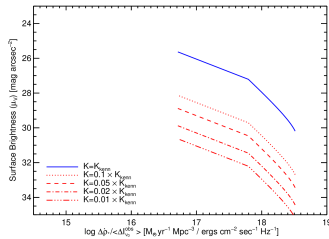
Figure 7.— Solid blue curve is the surface brightness ($\mu_{V}$) versus the differential comoving SFR density per intensity $\Delta\dot{\rho_{*}}/\Delta\langle I_{\nu_{0}}^{\rm obs}\rangle$ predicted for Kennicutt–Schmidt relation with $K=K_{\rm Kenn}$. The red curves depict what $\Delta\dot{\rho_{*}}/\Delta\langle I_{\nu_{0}}^{\rm obs}\rangle$ looks like for different values of the normalization constant $K$, where $K_{\rm Kenn}$=(2.5$\pm$0.5)$\times$10^-4 $M_{\odot}{\rm\ yr^{-1}\ kpc^{-2}}$ (Kennicutt, 1998a, b). The curves in this figure predict the amount of star formation that should be observed around LBGs for different efficiencies of star formation from Equations (25) and (26). The dotted line is for $K=0.1\times K_{\rm Kenn}$, the dashed line is for $K=0.05\times K_{\rm Kenn}$, the the dot-dashed line is for $K=0.02\times K_{\rm Kenn}$, and the tripple-dot-dashed line is for $K=0.01\times K_{\rm Kenn}$. The range of surface brightnesses corresponds to $5\times 10^{20}$ cm${}^{-2}<N<1\times 10^{22}$cm^-2.

The resulting predictions for the surface brightness, $\mu_{V}$, versus the differential comoving SFR density per intensity, $d\dot{\rho_{*}}/{d\langle I_{\nu_{0}}^{\rm obs}\rangle}$, is depicted by the blue curve in Figure 7. The red curves in this figure depict $d\dot{\rho_{*}}/{d\langle I_{\nu_{0}}^{\rm obs}\rangle}$ for different values of the normalization constant $K$, where $K_{\rm Kenn}$=(2.5$\pm$0.5)$\times$10^-4 $M_{\odot}{\rm\ yr^{-1}\ kpc^{-2}}$ (Kennicutt, 1998a, b). First, we note that $d\dot{\rho_{*}}/{d\langle I_{\nu_{0}}^{\rm obs}\rangle}$ for a given $K$ decreases as $\mu_{V}$ decreases because of the decreasing population of high column-density DLAs (i.e. DLAs with higher surface brightnesses). Second, we note that both $\dot{\rho_{*}}$ and ${\langle I_{\nu_{0}}^{\rm obs}\rangle}$ are linearly proportional to $K$, and therefore $K$ cancels out in the $x$-direction, leaving only the observed $\mu_{V}$ to vary with $K$ in the $y$-direction. We plot $\mu_{V}$ on the $y$-axis to conceptually facilitate the conversion of these results later in the paper and note that $d\dot{\rho_{*}}/{d\langle I_{\nu_{0}}^{\rm obs}\rangle}$ is a function of $N$ and therefore $\mu_{V}$. The curves in this figure predict the amount of star formation that should be observed around LBGs for different efficiencies of star formation, which will be compared to the data in Section 6.2. We plot $d\dot{\rho_{*}}/{d\langle I_{\nu_{0}}^{\rm obs}\rangle}$ for the range in $\mu_{V}$ that corresponds to $N_{\rm min}<N<N_{\rm max}$, where $N_{\rm min}=5\times 10^{20}$cm^-2, and $N_{\rm max}=1\times 10^{22}$ cm^-2. The value of $N_{\rm min}$ is lower than the range of threshold column densities of $N_{\perp}^{\rm crit}$ observed for nearby galaxies (Kennicutt, 1998b), but at a column density high enough such that we may start to see star formation occur. Also, recent results probing in the outer disks of nearby galaxies observe star formation at low column densities in atomic-dominated hydrogen gas (Fumagalli & Gavazzi, 2008; Bigiel et al., 2010b, a). Regardless, our measurements do not probe column densities down to this level, so the exact value for $N_{\rm min}$ does not affect the results.

6.2. Stacking Randomly Inclined Disks

We wish to compare these theoretical values of $d\dot{\rho_{*}}/{d\langle I_{\nu_{0}}^{\rm obs}\rangle}$, predicted for DLA gas forming stars according to the KS relation, to empirical measurements of $\Sigma_{\rm SFR}$ for our LBG sample. To do this, we require a method to convert the radial surface brightness profile in Figure 4 into $\mu_{V}$ versus $d\dot{\rho_{*}}/{d\langle I_{\nu_{0}}^{\rm obs}\rangle}$. For a given ring corresponding to a point in the radial surface brightness profile and covering an area $\Delta A$ we can calculate $\Delta\dot{\rho_{*}}$ from the measured intensity $\langle I_{\nu_{0}}^{\rm obs}\rangle$. $\Delta\dot{\rho_{*}}$ is similar to the differential $\dot{\rho_{*}}$ mentioned above, and is calculated from the flux measured in an annular ring at some radius from the center of the LBGs. Specifically,

$$\Delta\dot{\rho_{*}}=\frac{\Delta L_{\nu}N_{\rm LBG}}{C^{\prime}V_{\rm UDF}}\;,$$ (27)

where $C^{\prime}$ is the conversion factor from FUV radiation to SFR, $C^{\prime}=8\times 10^{27}$ erg s^-1 Hz^-1 ($M_{\odot}$ yr^-1)^-1, $\Delta L_{\nu}$ is the luminosity per unit frequency interval for a ring with area $\Delta A$, $N_{\rm LBG}$ is the number of $z\sim 3$ LBGs in the UDF, and $V_{\rm UDF}$ is the comoving volume of the UDF. As discussed in Section 3.1, we use a comoving volume of 26436 Mpc³. We recognize that $N_{\rm LBG}$ is dependent on the depth of images available to make selections, and discuss this completeness issue in Appendix A.3. The value of $\Delta\dot{\rho_{*}}$ depends on $\Delta L_{\nu}$, and therefore on the inclination angle $i$ for a given measured intensity, in the case of planes of preferred symmetry.

In order to determine $\Delta\dot{\rho_{*}}$, we average over all inclination angles in our determination of $\Delta L_{\nu}$, which depends on $\Sigma_{\nu}^{\perp}$ described in Section 5.2. Specifically, we use Equation (9) in conjunction with $\Delta L_{\nu}=\Delta A_{\perp}\Sigma_{\nu}^{\perp}$ to find $\Delta\dot{\rho_{*}}$, where $\Delta A_{\perp}$ is the area parallel to the plane of the disk. First, we rewrite $\Delta A_{\perp}$ in terms of $\Delta A$, the projection of $\Delta A_{\perp}$ perpendicular to the line of sight, and find that averaging over all inclination angles yields $\Delta A_{\perp}=2\Delta A$. We can then rewrite $\Delta A_{\perp}$ in terms of $\Delta\Omega$, the solid angle subtended by one of the rings from the surface brightness profile, and $\Delta A$, yielding $\Delta A_{\perp}=2\Delta\Omega d_{A}^{2}$. Using this relation, we find

$$\Delta\dot{\rho_{*}}=\frac{8\pi(1+z)^{3}{d_{A}}^{2}N_{\rm LBG}\Delta F_{\nu_{0}}^{\rm obs}(r)}{\ln(R/H)C^{\prime}V_{\rm UDF}}\;,$$ (28)

where $\Delta F_{\nu_{0}}^{\rm obs}(r)$ is the observed integrated flux in a ring as a function of the radius $r$. We then calculate the change in intensity from one ring to the next, $\Delta\langle I_{\nu_{0}}^{\rm obs}\rangle$, to get $\Delta\dot{\rho_{*}}/{\Delta\langle I_{\nu_{0}}^{\rm obs}\rangle}$ by measuring the intensity change across each ring by taking the difference between values of the intensity on either side of each point and dividing by two. In the case that $\Delta\langle I_{\nu_{0}}^{\rm obs}\rangle$ as calculated above is negative, we take the change in intensity over a larger interval.

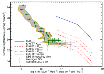
Figure 8.— Surface brightness ($\mu_{V}$) versus the differential comoving SFR density per intensity ($\Delta\dot{\rho_{*}}/\Delta\langle I_{\nu_{0}}^{\rm obs}\rangle$), comparing the measured emission in the outskirts of LBGs to the predicted levels for different SFR efficiencies. The blue and red lines are the predictions from Figure 7. The filled gray region represents observed emission in the outskirts of LBGs for a range in aspect ratios, with $R/H$ values ranging from 10 to 100, and the filled gold region is its 1$\sigma$ uncertainty. The green diamonds are the average value of the possible aspect ratios, with the error bars reflecting the measurement uncertainties (including the uncertainty due to the variance in the image composite).

Figure 8 shows a comparison of the theoretical model from Section 5.2.2 and the measured values from the radial surface brightness profile. The measurements are for a range in aspect ratios, with $R/H$ values from 10 to 100, similar to Section 5.2. We display the data in two complementary ways. First, the green diamonds depict results assuming the average value of the possible aspect ratios, with the error bars reflecting the measurement uncertainties (including the uncertainty due to the variance in the image composite) in order to portray the precision of our measurements. Second, we show a filled region, where the gray represent results for the full range in aspect ratios and the gold represents the 1$\sigma$ uncertainties on top of that range. This shows the region that is acceptable for each of those points. In both portrayals, we only include uncertainties of the aspect ratios, the variance due to stacking different LBGs, and the measurement uncertainties, and do not include uncertainties in the FUV light to SFR conversion factor ($C$) from Equation (4), or any other such systematic uncertainties. We truncate the data at a radius of $\sim 0.8$ arcsec ($\sim 6$ kpc) corresponding to a $3\sigma$ cut to include only measurements with high signal to noise. We note that in calculating the S/N values, we include the uncertainties due to the variance of objects in the composite stack. The data beyond a radius of $\sim 0.8$ arcsec are plotted in gray, and while they yield similar results, they are not included due to their low S/N.

The results shown in Figure 8 do not yet include completeness corrections, which we describe in Appendix A.3. We present the completeness corrected comparison between the theoretical models of $d\dot{\rho_{*}}/{d\langle I_{\nu_{0}}^{\rm obs}\rangle}$ for DLAs with measured values of $\Delta\dot{\rho_{*}}/{\Delta\langle I_{\nu_{0}}^{\rm obs}\rangle}$ in Figure 9. This shows that, under the hypothesis that the observed extended FUV emission comes from in situ star formation of DLA gas, the DLAs have an SFR efficiency at $z\sim 3$ significantly lower than that of local galaxies. In fact, the Kennicutt parameter $K$ needs to be reduced by a factor of 10–50 below the local value, $K=K_{\rm Kenn}$. The values of $\Delta\dot{\rho_{*}}/{\Delta\langle I_{\nu_{0}}^{\rm obs}\rangle}$ that intersect the predictions of the theoretical models for $N=5\times 10^{20}$–$1\times 10^{22}$ are black crosses and have S/N values ranging from $\sim$17 to $\sim$3 suggesting that the measurements are robust. These points correspond to radii of $\sim 0.4$–$0.8$ arcsec ($\sim 3$–$6$ kpc). The point with the largest value of $\Delta\dot{\rho_{*}}/{\Delta\langle I_{\nu_{0}}^{\rm obs}\rangle}$ of $\sim 17.4$ in Figure 9 seems to deviate from what otherwise would be a clear trend. This point corresponds to the point at a radius of $0.72$ arcsec in Figure 4, which also differs slightly from the general decreasing trend in $\mu_{V}$. However, it is consistent within their uncertainties for the surface brightness profile, and we are not concerned about it. All the points at radii larger than $\sim 0.8$ arcsec also intersect the theoretical models with similar efficiencies, but are not included as they have lower S/N. The values of $K$ vary for each data point and are not constant for a given $\mu_{V}$. These tantalizing results will be discussed in Section 7, and we consider the effects of stacking different samples of LBGs in Appendix B.

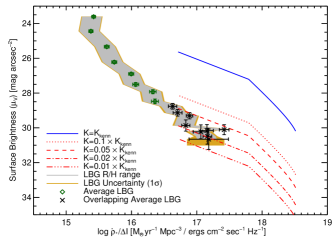
Figure 9.— Same as Figure 8, but corrected for completeness. The points that overlap with the theoretical models are now black crosses, to emphasize the points that will be used for the rest of this work. These points correspond to radii of 0.^′′405 through 0.^′′765. We omit the low S/N ($<3\sigma$) gray data points from Figure 8. By comparing the measurements in this plot to the predictions, we get the SFR efficiency for each surface brightness.

6.2.1 Variations in the KS Relation Slope $\beta$

The SFR efficiencies can also be decreased by lowering the slope $\beta$ of the KS relation, while keeping $K=K_{\rm Kenn}$. The value of $\beta$ in the literature ranges from $\beta\sim 1.0$ (Bigiel et al., 2008) to $\beta\sim 1.7$ (Bouché et al., 2007). Increasing the value of $\beta$ would increase the SFR efficiency, so we do not consider that here. On the other hand, lower values of $\beta$ would decrease the SFR efficiency and there are physical motivations to consider $\beta$ values as low as 1.0 (e.g., Elmegreen, 2002; Kravtsov, 2003). However, even reducing $\beta$ to values as low as 0.6 does not reduce the SFR efficiency enough to match our observations, and there are no physical motivations nor data to justify values of $\beta$ lower than 0.6. Lastly, decreasing the value of $\beta$ not only decreases the SFR efficiency, but it also decreases the value of $d\dot{\rho_{*}}/{d\langle I_{\nu_{0}}^{\rm obs}\rangle}$ (see Equation (25)). While decreasing $\beta$ would move the blue curve in Figure 9 down, it also moves it to the right and does not help the models match our observations. Therefore, we focus on other mechanisms for reducing the SFR efficiencies by varying the value of the parameter $K$.

6.3. The Kennicutt Schmidt Relation for Atomic-dominated Gas at High Redshift

As a tool to understand the low SFR efficiencies, and in order to compare our results to those of Wolfe & Chen (2006) and Bigiel et al. (2010b), and simulations such as those by Gnedin & Kravtsov (2010), we translate the result from Section 6.2 and Figure 9 to a common set of parameters to obtain a plot of $\Sigma_{\rm SFR}$ versus $\Sigma_{\rm gas}$. We derive this conversion for the emission in the outskirts of LBGs in Section 6.3.1, and for the DLA upper limits from Wolfe & Chen (2006) in Section 6.3.2.

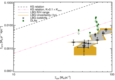
Figure 10.— Star formation rate per unit area ($\Sigma_{\rm SFR}$) versus gas density ($\Sigma_{\rm gas}$). The dashed line represents the KS relation with $K=K_{\rm Kenn}$=(2.5$\pm$0.5)$\times$10^-4 $M_{\odot}{\rm\ yr^{-1}\ kpc^{-2}}$, while the triple dot-dashed line is for $K=0.1\times K_{\rm Kenn}$. The gray filled region, the gold filled region, and the black crosses represent the same data as in Figure 9. The green data points corresponding to upper limits derived for DLAs without central bulges of star formation from Wolfe & Chen (2006) converted to work with this plot. Since DLA sizes are not known, the upper limits are derived for angular diameters $\theta_{\rm kern}$=4^′′, 2^′′, 1^′′, 0.^′′6, 0.^′′5, 0.^′′4, 0.^′′3, and 0.^′′25, from left to right. The data all fall at or below 10% of the KS relation, showing a lower SFR efficiency than predicted.

6.3.1 Converting the LBG Results to $\Sigma_{\rm SFR}$ versus $\Sigma_{\rm gas}$

We calculate $\Sigma_{\rm SFR}$ directly using Equation (4), where the average intensity is obtained from the radial surface brightness profile of the composite LBG stack in rings as explained in Section 4.3 (Figure 4). As $\mu_{V}$ algebraically increases with increasing radius, $\Sigma_{\rm SFR}$ will generally decrease with increasing radius. We compute $\Sigma_{\rm gas}$ by first inferring the value of $K$ for each data point that intersects the theoretical curves in the $\mu_{V}$ versus $\Delta\dot{\rho_{*}}/{\Delta\langle I_{\nu_{0}}^{\rm obs}\rangle}$ plane, since each theoretical curve is parameterized by a fixed value of $K$. We precisely find the corresponding efficiency by calculating a grid of models with $K$ varying by 0.001. We then use this value of $K$ and the KS relation (Equation (2)) to calculate $\Sigma_{\rm gas}$ for each value of $\Sigma_{\rm SFR}$ inferred from the measured $\mu_{V}$.

In short, we directly measure $\Sigma_{\rm SFR}$ through the emitted FUV radiation, and then calculate $\Sigma_{\rm gas}$ for the corresponding $K$ that matches the DLA model. We note that $\Sigma_{\rm SFR}$ is a direct measurement, while $\Sigma_{\rm gas}$ comes from the DLA model which is based on the column-density distribution function of DLA gas. The result is shown in Figure 10, which plots $\Sigma_{\rm SFR}$ versus $\Sigma_{\rm gas}$. We truncate the plot to include only data that overlaps with observed DLA gas densities, namely $N\leq 1\times 10^{22}$ cm^-2, where $N$ is calculated from Equation (3) using the $K$ value determined for that $\mu_{V}$. The dashed line black represents the KS relation with $K=K_{\rm Kenn}$=(2.5$\pm$0.5)$\times$10^-4 $M_{\odot}{\rm\ yr^{-1}\ kpc^{-2}}$, while the pink triple dot-dashed line represents $K=0.1\times K_{\rm Kenn}$. The gray filled area with the 1$\sigma$ uncertainty and the black points represent the same data as in Figure 9. The green upper limits will be described in Section 6.3.2.

The LBG outskirts in Figure 10 clearly have lower SFR efficiencies than predicted by the KS relation. In addition, they appear to follow a power law that is steeper than the KS relation at low redshift. However, there is a large scatter caused by the uncertainty introduced by the sky-subtraction uncertainty (see Section 4.2), and the sample variance due to stacking different objects (see Section 4.3). We are therefore cautious about fitting a power law to this data by itself, and investigate this trend further in Section 7.3.1.

6.3.2 Converting DLA Data to $\Sigma_{\rm SFR}$ versus $\Sigma_{\rm gas}$

To convert the DLA points from Wolfe & Chen (2006), we use the same idea as that of the LBG data, except that in this case we do not have detected star formation, and therefore we use upper limits. Also, rather than using the new framework developed above, we use the formalism developed for DLAs without central bulges of star formation (Wolfe & Chen, 2006). We start with Figure 7 of Wolfe & Chen (2006), which basically plots the SFR density due to star formation in neutral atomic-dominated hydrogen gas (i.e., DLAs) with column densities greater than $N$ ($\dot{\rho_{*}}(>N)$) versus $\mu_{V}$. Similar to our Figure 9, Figure 7 of Wolfe & Chen (2006) has DLA models with different Kennicutt parameters $K$. We follow the same technique of using the intersection of these models with the data to find $K$ values for each $\mu_{V}$. However, in this case the values of $\mu_{V}$ do not correspond to detected surface brightnesses of LBGs, but rather correspond to threshold surface brightnesses, i.e., the lowest values of $\langle I_{\nu_{0}}^{\rm obs}\rangle$ that would be measured for a DLA of a given angular diameter. Therefore, we cannot calculate $\Sigma_{\rm SFR}$ the same way as in Section 6.3.1.

To determine $\Sigma_{\rm SFR}$, we first calculate an effective minimum column density, $N_{\rm eff}$, corresponding to the threshold surface brightness of Wolfe & Chen (2006). We do this using the $K$ values from the intersection points, the thresholds $\mu_{V}$, and Equation 3. We then calculate $\Sigma_{\rm SFR}$, the average over all possible column densities above $N_{\rm eff}$, as

$$\Sigma_{\rm SFR}=\langle\Sigma_{\rm SFR}(>N_{\rm eff})\rangle=\frac{c}{H_{0}}\frac{\dot{\rho_{*}}(>N_{\rm eff})}{{\int_{N_{\rm eff}}^{N_{\rm max}}J(N^{\prime})dN^{\prime}}}\;,$$ (29)

where $J(N)$ is the integral in Equation (14). We then calculate $\Sigma_{\rm gas}$ using these $\Sigma_{\rm SFR}$, the above $K$ values, and Equation (2). The resulting values are overlaid on the LBG results in Figure 10. We emphasize that the two results are independent tests. The DLA upper limits put constraints on the KS relation in the case of no central bulge of star formation, while the LBG outskirts data put constraints on in situ star formation in DLAs associated with LBGs. Together, these results show that the SFR efficiency in diffuse atomic-dominated gas at $z\sim 3$ is less efficient than predicted by the KS relation for local galaxies.

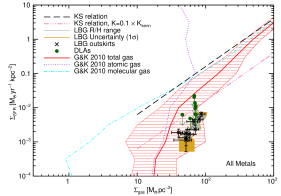
Figure 11.— Star formation rate per unit area ($\Sigma_{\rm SFR}$) versus gas density ($\Sigma_{\rm gas}$) for both the data as shown in Figure 10, and the KS relation for simulated galaxies at $z=3$ from (Gnedin et al., 2009). The left panel includes gas of all metallicities while the right panel considers only the gas with metallicities below $0.1Z_{\odot}$. The solid red and blue lines are the mean relation for the total neutral-gas surface density (atomic and molecular) and the hatched area shows the rms scatter around the mean. The dotted purple line shows the mean KS relation only considering the atomic gas, while the dot-dashed cyan line shows it for the molecular gas. The long-dashed line is the Kennicutt relation for local ($z\sim 0$) galaxies (Kennicutt, 1998a), while the triple-dot-dashed line is for $K=0.1\times K_{\rm Kenn}$. The gray and gold lines and the black and green points are the data and are the same as in Figure 10.

7. Discussion of Results

We present, for the first time, evidence for LSB emission around LBGs on spatial scales large compared to the LBG cores due to in situ star formation in gas associated with LBGs (see Figure 4). Using the theoretical framework developed in Section 6.1.2, we model this emission as the average in situ star formation in atomic-dominated gas surrounding LBGs at $z\sim 3$. Since most of the atomic-dominated gas at high redshift is in DLAs, we assume that this is DLA gas. We find that under this hypothesis, the efficiency of star formation in the atomic-dominated gas is significantly lower than what is expected for predictions by the KS relation. This is clearly evident in Figure 10, which compares the local KS relation directly to the observations. The efficiency of in situ star formation in atomic-dominated gas appears to be a factor of $10$–$50$ lower than that of local galaxies that follow KS relation. In addition, the SFR efficiency of atomic-dominated gas around galaxies without bright cores is constrained by the thresholds measured by Wolfe & Chen (2006), who impose similar efficiencies on the in situ star formation in DLAs, as shown by the green upper limits in Figure 10. Therefore, together with the results from Wolfe & Chen (2006), we constrain the SFR efficiency of all neutral atomic-dominated hydrogen gas (DLAs) at $z\sim 3$.

There are multiple possible effects contributing to the observed lower SFR efficiencies, including a higher background radiation field at high redshift, low-metallicity of DLAs, and the role of molecular versus atomic hydrogen in star formation. We start the discussion by comparing our results to the models of low-metallicity high-redshift galaxies by Gnedin & Kravtsov (2010) in Section 7.1. We then consider the roles of molecular and atomic-dominated gas in the KS relation in the context of the saturation of atomic dominated in Section 7.2. We investigate whether there is a variation of the KS relation with redshift in Section 7.3, and compare our results at high redshift with those in the outer disks of local galaxies in Section 7.3.1. We then consider the effect that a bimodality of the DLA population would have on the results in Section 7.4, and a caveat on the results based on DLA sizes in Section 7.5. Lastly, we address the “Missing Metals” problem of DLAs in Section 7.6.

7.1. Models of the Kennicutt Schmidt Relation in High-redshift Galaxies

Here we discuss two effects contributing to the observed lower efficiencies: First, at higher redshifts the background radiation field (Haardt & Madau, 1996) is stronger, yielding a higher UV-flux environment. This photodissociates the molecular hydrogen ($\rm H_{2}$) content of the gas, raising the threshold for the gas to become molecular, therefore requiring higher gas densities to form stars. Second, the metallicity of DLAs at high redshift is considerably lower than solar (Pettini et al., 1994, 1995, 1997, 2002a; Prochaska et al., 2003), and therefore has a lower dust content, which is needed to form molecular hydrogen and to shield the gas from photodissociating radiation.

Recent theoretical work (Krumholz et al., 2008; Gnedin et al., 2009; Krumholz et al., 2009b, a; Gnedin & Kravtsov, 2010, 2011) suggests that the most important part in determining the amplitude and slope of the KS relation is the dust abundance, and therefore the metallicity. Gnedin & Kravtsov (2010) investigate the KS relation at high redshift using their metallicity dependent model of molecular hydrogen (Gnedin et al., 2009). They find that while the higher UV flux does lower the SFR, it also lowers the surface density of the neutral gas, leaving the KS relation mostly unaffected. However, they find that the lower metallicity, and therefore lower dust-to-gas ratio, causes a steepening and lower amplitude in the KS relation. This yields lower molecular gas fractions, which in turn reduces SFR for a given gas surface density, $\Sigma_{\rm gas}$. This would yield lower observed SFR efficiencies similar to what is measured in this study.

We compare our results with the $z=3$ model KS relation (Gnedin & Kravtsov, 2010) in Figure 11, with a plot showing our data overlaid with the model results, and find that their predictions are consistent with our findings. This plot is similar to Figure 3 in Gnedin & Kravtsov (2010), as we provided them with our preliminary results for comparison. However, there was previously an error in our implementation of the theoretical framework, yielding slightly different results than presented here. Also, here we split the figure into two panels, with the left panel including gas of all metallicities for galaxies at $z=3$, and the right panel including only the gas with metallicities below $0.1Z_{\odot}$. Each plot includes the same points as shown in Figure 10. In addition, the plots show the KS relation for the simulated galaxies at $z=3$ for the total neutral gas (atomic and molecular), with the solid lines showing the mean value and the hatched area showing the rms scatter around the mean. The dotted purple line shows the mean KS relation only considering the atomic gas, while the dot-dashed cyan line shows it for the molecular gas. The dashed black line is the best-fit relation of Kennicutt (1998a) for $z\sim 0$ galaxies, while the triple dot-dashed line is for $K=0.1\times K_{\rm Kenn}$. The blue line in the right panel is closer to the range of observed metallicities observed in DLAs of $\sim 0.04Z_{\odot}$ (Prochaska et al., 2003, ; M. Rafelski et al. 2011 in preparation). The use of a metallicity cut of $0.1Z_{\odot}$ is reasonable, since the mass-weighted and volume-weighted metallicity of the atomic gas is $\sim 0.02Z_{\odot}$ and $\sim 0.03Z_{\odot}$ respectively (N. Gnedin 2010, private communication), matching the observed DLA metallicities nicely. In addition, although the dispersion of DLA metallicities is large, the majority of DLAs have metallicities below 0.1 $Z_{\odot}$, making this a good choice for a cut to compare to DLA gas.

The spatially extended emission around LBGs is consistent with both the total and low-metallicity gas models in Figure 11. While the uncertainties in both the model and the data are large, taking the results at face value, we can gain insights into the nature of the gas reservoirs around LBGs. The data are a better match to the model with the metallicity cut of $0.1Z_{\odot}$, coinciding with the mean relation for this model. On the other hand, the emission from gas around LBGs is also consistent within the 1$\sigma$ uncertainties of the model including gas with all metallicities for the part of the rms scatter below the mean. This lower part of the hatched area in the left panel of Figure 11 represents the gas at the lower end of the metallicity distribution shown in Gnedin et al. (2009), having a mass-weighted and volume-weighted metallicity of the atomic gas of $\sim 0.26$ $Z_{\odot}$ (N. Gnedin 2010, private communication), which is consistent with that of $z=3$ galaxies having an average metallicity of $\sim 0.25$ $Z_{\odot}$ (Shapley et al., 2003; Mannucci et al., 2009). Since the observations fall below the mean model for the higher metallicity model, and coincide with the model for the lower metallicity model, we conclude that the metallicity of the gas is most likely around the mean metallicity of the low-metallicity model, $\sim 0.04Z_{\odot}$, and is definitely below $\sim 0.26$ $Z_{\odot}$, the metallicity of the model including gas of all metallicities The results therefore imply that the gas in the outskirts of LBGs has lower metallicities than the LBG cores. In fact, the observed SFRs and the implied metallicities from the models are fully consistent with the outer regions of LBGs consisting of DLA gas.

7.2. The Roles of Molecular and Atomic-dominated Gas in the Kennicutt Schmidt Relation

The reduction in SFR efficiency will also be affected by the competing roles played by atomic and molecular gas in the KS relation. There has been some debate as to whether the KS relation should include both atomic and molecular gas. All stars are believed to form from molecular gas, and some workers argue that $\Sigma_{\rm SFR}$ correlates better with molecular gas than atomic gas (Wong & Blitz, 2002; Kennicutt et al., 2007; Bigiel et al., 2008). On the other hand, other observations show a clear correlation of the total gas surface density, $\Sigma_{\rm gas}$, with $\Sigma_{\rm SFR}$ (Kennicutt, 1989, 1998a; Schuster et al., 2007; Crosthwaite & Turner, 2007), and the atomic gas surface density, $\Sigma_{\rm HI}$, with $\Sigma_{\rm SFR}$ (Bigiel et al., 2010b).

These differences can be understood in the context of the saturation of atomic-dominated gas at high column densities. Above a specified threshold of $\Sigma_{\rm HI}$, the atomic gas is converted into molecular gas and no longer correlates with $\Sigma_{\rm SFR}$. This saturation of atomic hydrogen gas above a threshold surface density is clearly observed (see Figure 8 of Bigiel et al., 2008) for local galaxies at $z=0$, and occurs at surface densities of $\sim 10$$M_{\odot}$ pc^-2 (Wong & Blitz, 2002; Bigiel et al., 2008). However, below this threshold surface density, there is a correlation of $\Sigma_{\rm HI}$ and $\Sigma_{\rm SFR}$. This is most clearly seen in the results analyzing the outer disks of nearby galaxies (Bigiel et al., 2010b), where a clear correlation of $\Sigma_{\rm HI}$ with $\Sigma_{\rm SFR}$ is observed. In fact, they find that the key regulating quantity for star formation in outer disks is the column density of atomic gas. Further evidence is seen in the outskirts of M83, where the distribution of FUV flux again follows the $\Sigma_{\rm HI}$ (Bigiel et al., 2010a). In fact, Bigiel et al. (2010a) find that in the outskirts of M83, massive star formation proceeds almost everywhere H I is observed. While these outer disks must contain some molecular gas in order for star formation to occur, they are nonetheless dominated by atomic gas with surface densities lower than the saturation threshold seen in Bigiel et al. (2008).

The saturation of atomic gas above a threshold surface density is investigated in theoretical models (Krumholz et al., 2009a; Gnedin & Kravtsov, 2010, 2011), which reproduce the saturation threshold for atomic gas in local galaxies. Moreover, the authors find that the threshold surface density for saturation varies with metallicity, where lower metallicity systems have higher thresholds (see Figure 4 of Krumholz et al., 2009a). In addition, the simulations of $z=3$ galaxies by Gnedin & Kravtsov (2010) show an increased saturation surface density of atomic gas of $\sim 50$$M_{\odot}$ pc^-2, as seen in the purple dotted line in Figure 11. The line clearly saturates, with no clear relation between $\Sigma_{\rm HI}$ and $\Sigma_{\rm SFR}$ above $\sim 50$$M_{\odot}$ pc^-2, but with a clear relation below this density. Since $z=3$ galaxies are typically LBGs with metallicities of $\sim 0.25Z_{\odot}$ (Shapley et al., 2003; Mannucci et al., 2009), this is consistent with predictions from Krumholz et al. (2009a). The model with only lower metallicity gas (right panel of Figure 11) saturates at even higher atomic gas surface densities (Gnedin & Kravtsov, 2010), continuing the relation of the threshold saturation of $\Sigma_{\rm HI}$ with metallicity. It appears that $\Sigma_{\rm HI}$ tracks $\Sigma_{\rm gas}$ to large values of $\Sigma_{\rm SFR}$, and no saturation occurs in $\Sigma_{\rm HI}$ until $\sim$ 200–300 $M_{\odot}$ pc^-2.

Comparison of the saturation thresholds found by Gnedin & Kravtsov (2010) with our data in the right panel of Figure 11 reveals that the data are below this threshold for saturation of atomic gas for all values of $\Sigma_{\rm HI}$ for the model with the 0.1$Z_{\odot}$ cut, which most closely matches our results. We therefore conclude that the measured decrease in SFR efficiency is not due to the saturation of atomic-dominated gas. In fact, our data confirm that the atomic-dominated gas does not saturate for $\Sigma_{\rm HI}$ of at least $\gtrsim 100$$M_{\odot}$ pc^-2. This number is larger than predicted for LBG metallicities, yet smaller than predicted for DLA metallicities. This suggests that the average metallicity of the gas in the outskirts of LBGs is between $0.1Z_{\odot}$ and $0.25Z_{\odot}$. This is consistent with the metallicity estimate made in Section 5.4 of $0.12Z_{\odot}$ to $0.19Z_{\odot}$ based on the metal production rate of star formation.

While molecular gas is very likely needed to form stars, it is also clear from results for local outer disks (Bigiel et al., 2010b) and our results at high redshift that star formation can be observed even when molecular gas does not dominate azimuthal averages in rings of galactic dimensions. We do not suggest that stars are forming from purely atomic gas, but rather that in the presence of high density atomic gas, there are sufficient molecules to cool the gas such that star formation can be initiated by gravitational collapse. We predict that more sensitive measurements of molecular gas in local outer disks would result in the detection of molecular gas. On the other hand, recent models by Low & Glover (2010) suggest that molecular hydrogen may not be the cause of star formation, but rather a consequence of the star formation. In this scenario, CO traces dense gas that is already gravitationally unstable and would probably form stars regardless. More investigations are needed to better understand what is fundamentally required for star formation, and our work provides some observational constraints for such work.

We note that even though large amounts of molecular gas are not observed in DLAs (Curran et al., 2003, 2004), the molecular gas has a very small covering fraction, and therefore is unlikely to be seen along random sight lines (Zwaan & Prochaska, 2006). We also note that Bigiel et al. (2010b) find that the FUV emission reflects the recently formed stars without large biases from external extinction. We similarly do not expect much extinction in the outer parts of the LBGs, as DLAs have low dust-to-gas ratios (Pettini, 2004; Frank & Péroux, 2010). Therefore, unless the gas in the outskirts of LBGs is due to star formation in molecular-dominated gas, we do not expect large extinction corrections to be necessary.

7.3. Is There a Variation of the Kennicutt Schmidt Relation with Redshift?

Recent studies of star-forming galaxies at high redshift have suggested that the KS relation does not vary with redshift (Bouché et al., 2007; Tacconi et al., 2010; Daddi et al., 2010; Genzel et al., 2010). These studies do a careful job of comparing $\Sigma_{\rm SFR}$ and the molecular gas surface density, $\Sigma_{\rm H_{2}}$, of high- and low-redshift systems, and find that the galaxies fit a single KS relation. This is starkly different than our finding a lower SFR efficiency at high redshift. Furthermore, these studies differ from simulations of high-redshift galaxies that do find a reduced SFR efficiency (Gnedin & Kravtsov, 2010).

These differences may be due to comparisons of different types of gas. In our results, we consider atomic-dominated gas as found in DLAs, while the other observational studies are focused on molecular-dominated gas with galaxies having high molecular fractions and higher metal abundances. Similarly, Bigiel et al. (2010b) also found a lower SFR efficiency in the outskirts of otherwise normal local galaxies when probing atomic-dominated gas. There are two different possible scenarios that explain the results. First, the KS relation for atomic-dominated gas follows a different KS relation than the KS relation for molecular-dominated gas. This possibility would explain the observed lower efficiencies of star formation in (1) the outskirts of $z\sim 3$ LBGs as measured here, (2) the DLAs without star-forming bulges as measured by Wolfe & Chen (2006), and (3) the outskirts of local galaxies as measured by Bigiel et al. (2010b).

On the other hand, the simulations by Gnedin & Kravtsov (2010) focus on galaxies with low metallicities similar to those observed of LBGs ($\sim 0.26$ $Z_{\odot}$) and find reduced SFR efficiencies in both their molecular-dominated and their atomic-dominated gas. They also find that the efficiency is directly related to the metallicity of the gas, suggesting that the decreased star formation efficiency is most likely due to decreased metallicities. These models accurately predict the SFR efficiencies we measure in the outskirts of the LBGs if they are associated with DLAs. The outskirts of the local galaxies measured by Bigiel et al. (2010b) are also generally of lower metallicities (e.g. de Paz et al., 2007; Cioni, 2009; Bresolin et al., 2009), so the decreased efficiencies could also be due to the lower metallicity. The SFR efficiencies in Bigiel et al. (2010b) are similar to this study, and we discuss this below in Section 7.3.1.

In addition, Bigiel et al. (2010a) find a clear correlation of the FUV light (representing star formation) with the location of the H I gas in M83. In the inner region they find a much steeper radial decline in $\Sigma_{\rm SFR}$ than in $\Sigma_{\rm H_{I}}$, while in the outer region of the disk, $\Sigma_{\rm SFR}$ declines less steeply, if at all (see Figure 4 of Bigiel et al., 2010a). Similarly, the metallicity in the inner part of M83 drops pretty steeply and then flattens out at larger radii (Bresolin et al., 2009). These results are consistent with the scenario that the metallicity is driving the efficiency of the SFR.

While it is not yet clear what causes the decrease in SFR efficiency in DLAs, the results suggest it is either due to a different KS relation for atomic-dominated gas or due to the metallicity of the gas rather than the redshift. Given the excellent agreement of our results with the predictions by Gnedin & Kravtsov (2010), and the suggestive results of the outer regions of M83, we give extra credence to the metallicities driving the SFR efficiencies. In fact, these two effects may be the same, as the outskirts of galaxies generally probably have lower metallicities, and therefore lower SFR efficiencies. While all the gas at high redshift may not have a reduced efficiency, care must be taken when using the KS relation in cosmological models, as the properties of gas vary with redshift, thereby affecting the SFR efficiencies.

Figure 12.— Star formation rate per unit area ($\Sigma_{\rm SFR}$) versus gas density ($\Sigma_{\rm gas}$) for the data as shown in Figure 10 and the results from the outer regions of spiral galaxies from (Bigiel et al., 2010b). The blue diamonds represent the best estimate for the true relation of $\Sigma_{\rm SFR}$ and $\Sigma_{\rm HI}$ from Bigiel et al. (2010b) accounting for their sensitivity, and the error bars represent the scatter. These points have been converted to use the same IMF and FUV–SFR conversion as used in this work. The long dashed line is the Kennicutt relation for local ($z\sim 0$) galaxies (Kennicutt, 1998a). The gray and gold lines and the black points are the data as shown in Figure 10. The dotted red line represents a power-law fit to the data with both the normalization and the slope as free parameters, and the green dot-dashed line is a power-law fit with the slope set to $\beta=1.4$, as described in Section 7.3.1.

7.3.1 Comparison of the $z\sim 3$ SFR Efficiency with Local $z=0$ Outer Disks

The environment for star formation at large galactic radii is significantly different than in the inner regions of star-forming galaxies, having lower metallicities and dust abundances, consisting of more H I than H₂ gas, and being spread out over large volumes. These environmental factors undoubtedly have effects on the conversion of gas into stars, and perhaps the SFR efficiency. Similar to our results at high redshift, the SFR efficiency in the local ($z=0$) outer disks is also less efficient than the KS relation (Bigiel et al., 2010b). Figure 12 plots our results of H I dominated gas in the outskirts of LBGs at $z\sim 3$ from Figure 10, in conjunction with the measurements of Bigiel et al. (2010b) of the outskirts of local spiral galaxies. These measurements combine data from the H I Nearby Galaxy Survey and the GALEX Nearby Galaxy Survey to measure both the atomic hydrogen gas surface density and the FUV emission tracing the SFR in 17 spiral galaxies. The blue diamonds in Figure 12 represent the best estimate for the true relation of $\Sigma_{\rm SFR}$ and $\Sigma_{\rm HI}$ from Bigiel et al. (2010b) accounting for their sensitivity, and the error bars represent the scatter in the measurements. The SFRs determined in Bigiel et al. (2010b) from the FUV luminosity use a Kroupa-type initial mass function (IMF) and the Salim et al. (2007) FUV–SFR calibration, while we use a Salpeter IMF and the FUV–SFR calibration from Madau et al. (1998) and Kennicutt (1998b). For comparison with our LBG results, we convert the SFRs from Bigiel et al. (2010b) to Salpeter by multiplying by a factor of 1.59 and to the Kennicutt (1998b) FUV–SFR calibration by multiplying by a factor of 1.30.

While these populations probe very different redshifts and gas densities, they both probe diffuse atomic-dominated gas in the outskirts of galaxies and have low metallicities. In fact, the differing redshifts enable a comparison of drastically different gas surface densities not possible at low redshift alone, due to the saturation of H I gas above a threshold surface density as described in Section 7.2. Specifically, Bigiel et al. (2010b) cannot probe significantly higher gas densities, as at $z=0$ the H I gas saturates at threshold surface densities of $\sim 10$$M_{\odot}$ pc^-2 (see Figure 8 in Bigiel et al., 2008). On the other hand, as described in Section 7.2, at $z\sim 3$ the H I gas does not saturate until much higher gas surface densities. However, our measurements at $z\sim 3$ are also limited in the other direction, as we cannot probe lower gas surface densities due to insufficient surface-brightness sensitivity, and therefore we are left with non-overlapping results for $10M_{\odot}$pc${}^{2}\lesssim\Sigma_{\rm gas}\lesssim 30$$M_{\odot}$pc².

It is not likely a coincidence that the SFR is less efficient in the outer regions of galaxies at both low and high redshifts. It may be that the SFR is less efficient in the outer regions of galaxies at all redshifts, and this possibility needs to be investigated. There is evidence that the metallicities in the inner regions of galaxies observed in emission are higher than that in the outer parts sampled by quasar absorption line systems at $z\sim 0.6$ (Chen et al., 2005, 2007). If the SFR efficiency depends on the metallicity, then we would expect lower efficiencies in the outer parts of these $z\sim 0.6$ galaxies as observed.

Comparing the data at low redshift with those at high redshift, we find that they appear to fall on a straight line in log space. We therefore fit a power law to the outer disk measurements in Figure 12, using the KS relation in Equation (2) and setting $\Sigma_{\rm c}=1~{}$$M_{\odot}$pc^-2. Leaving both the normalization and the slope as free parameters, our least-squares solution results in a normalization of $K=(1.4\pm 0.7)\times 10^{-5}$ $M_{\odot}{\rm\ yr^{-1}\ kpc^{-2}}$ and a slope of ${\beta}$=1.3$\pm$0.1, and is plotted as a dotted red line in Figure 12. In addition, we also fit a power law where we set the slope to the same value as in the KS relation (Kennicutt, 1998a, b), namely ${\beta}$=1.4. This fit has a normalization of $K=(8.5\pm 0.7)\times 10^{-6}$ $M_{\odot}{\rm\ yr^{-1}\ kpc^{-2}}$ and is plotted as a dot-dashed green line in Figure 12. The fit is consistent for both the low- and high-redshift galaxy outskirts, and the normalization is significantly lower than that of the KS relation, with a $K$ value that is 0.03 times the local value. We note that the slope of the LBG outskirts is larger than the slope for the outskirts of local galaxies. The metallicities of the outskirts of local galaxies are probably somewhat higher than those in the outskirts of LBGs, assuming they consist of DLA gas, and therefore this difference may be a result of differing metallicities.

We acknowledge that we may be comparing different environments when considering the high and low redshift outer disks, but they may be similar enough to tell us about star formation in the outskirts of galaxies. Indeed, both populations exhibit similar SFR efficiencies. Measurements of the SFR efficiency across a range of redshifts are needed to further explore if variations of the slope are real and evolve over time.

7.4. Bimodality of DLAs

There is evidence to suggest that there are two populations of DLAs (high cool and low cool), since the distribution of cooling rates of DLAs is bimodal (Wolfe et al., 2008). These two populations have significant differences in their cooling rates (and therefore SFRs), velocity widths, metallicity, dust-to-gas ratio, and Si II equivalent widths. The gas in the high cool population cannot be heated by background and/or in situ star formation alone, and so Wolfe et al. (2008) suggest that the high cool population is associated with compact star-forming bulges, or LBGs. These high cool DLAs typically have metallicities ($Z=0.09\pm 0.03~{}Z_{\odot}$), higher than the average for DLAs (Wolfe et al., 2008). The low cool population may also be associated with LBGs, although it is possible that this population is heated solely by in situ star formation. These low cool DLAs generally have lower than average metallicities ($Z=0.02\pm 0.01~{}Z_{\odot}$; Wolfe et al., 2008).

Given that our measurements in the outskirts of LBGs are consistent with both metallicities, it is possible that all DLAs are in the outskirts of LBGs. Alternatively, it would also be logical to associate the high cool population of DLAs with the gas responsible for the star formation in the outskirts of the LBGs, and the low cool population would then naturally be represented by the DLA upper limits from Wolfe & Chen (2006). While those DLAs are also likely associated with galaxies, their lower surface brightness may result in this being included in the Wolfe & Chen (2006) sample.

If we are mainly probing the high cool DLAs with the extended LSB emission around LBGs, and are mainly probing the low cool DLAs in the upper limits from Wolfe et al. (2008), then the number count statistics would need to be modified to account for the different percentages of high cool and low cool DLAs. However, these percentages are not yet very well constrained. A reasonable first try to modify the DLA models is to use the current observational result that about half the DLAs are high cool and half are low cool. If only high cool DLAs are included, it would lower the expected $\dot{\rho_{*}}$, which would increase the efficiencies of the SFR, moving the data to the left in Figure 11. Assuming that each of the two DLA populations represents half the DLAs, we find the data move to the left by about $\sim 0.1$ dex. This does slightly worsen the agreement of the outskirts of LBGs with the blue low metallicity model, but not by much. Also, in this scenario, the gas would have higher metallicities ($Z\sim 0.09$), and therefore we would expect the outskirts of the LBGs to fall to the left of the blue line. Regardless, the uncertainties in the models and the data are large enough that they could be compatible with a wide range of interpretations. In short, our SFR efficiency results do not drastically change whether or not there is a bimodality in the DLA population.

7.5. Effects of Different DLA Sizes

One caveat remains, which is the possibility that if DLAs are not associated with LBGs, and the FWHM linear diameters of DLAs at $z\sim 3$ are less than 1.9 kpc, then we have not put a limit on the in situ star formation in DLAs. However, as discussed in §3.1 of Wolfe & Chen (2006), all models suggested so far predict that the bulk of DLAs will have diameters larger than 1.9 kpc (e.g., Prochaska & Wolfe, 1997; Mo et al., 1998; Haehnelt et al., 2000; Boissier et al., 2003; Nagamine et al., 2006, 2007; Tescari et al., 2009; Hong et al., 2010), which is in agreement with the observations (Wolfe et al., 2005; Cooke et al., 2010). Rauch et al. (2008) find spatially extended Ly-$\alpha$ emission from objects with radii up to 4^′′ ($\sim$30kpc) and mean radii of $\sim 1$^′′ ($\sim$8 kpc) which they argue corresponds to the H I diameters of DLAs. While continuum emission has not been detected on these scales, it may have been observed from associated compact objects. In fact, almost all of the Ly-$\alpha$ selected objects have at least one plausible continuum counterpart (M. Rauch, 2010, private communication).

If we assume that the sources of Ly-$\alpha$ photons are distributed throughout the gas, then we can compare the $\Sigma_{\rm SFR}$ values from Rauch et al. (2008) to ours. In this scenario, the in situ star formation in the DLA gas is the source of the Ly-$\alpha$ photons, which is possibly associated with LBGs detected in the continuum. We note that currently there is no evidence for this assumption, and it is counter to the interpretation by Rauch et al. (2008), who assume that Ly-$\alpha$ radiation originates in a compact object embedded in the more extended DLA gas. On the other hand, we cannot rule out this possibility and it is intriguing, so we consider it here. Using the median size of their measured extended Ly$\alpha$ emission of $\sim 1$^′′, we convert their SFRs to $\Sigma_{\rm SFR}$ of 4$\times$10^-4 – 8$\times$10^-3 $M_{\odot}$ yr^-1 kpc^-2. This range in $\Sigma_{\rm SFR}$ overlaps our measured $\Sigma_{\rm SFR}$ shown in Figures 4 and 10, suggesting that we may be measuring the same star formation in DLAs in two very different methods. If this is the case, then the sizes of DLAs may be even larger than otherwise expected. Whether or not this interpretation is correct, we are definitely above the minimum size probed by Wolfe & Chen (2006) of 1.9 kpc, implying that the above mentioned caveat is unimportant. We are therefore confident that we have shown in Section 5 and Section 6 that the SFR efficiency in diffuse atomic-dominated gas at $z\sim 3$ is less efficient than for local galaxies.

7.6. The “Missing Metals” Problem

The metal production by LBGs can be compared to the metals observed in DLAs. Previously, the metal content produced in LBGs was found to be significantly larger than that observed in DLAs by a factor of 10 and was called the “Missing Metals” problem for DLAs (Pettini, 1999, 2004, 2006; Pagel, 2002; Wolfe et al., 2003a; Bouché et al., 2005). However, Wolfe & Chen (2006) found that when taking into account a reduced efficiency of star formation as found in DLAs at $z\sim 3$, then the metal over production by a factor of 10 changed to one of underproduction by a factor of three.

In this study, we calculated the metal production in the outskirts of LBGs and found that the metals produced there yield metallicities in the range of $0.12\pm 0.05Z_{\odot}$ to $0.19\pm 0.07Z_{\odot}$, depending on the outer radius for the integration of the SFR (see Section 5.3 and Table 2). The average metallicity of DLAs at $z\sim 3$ is $Z\sim 0.04Z_{\odot}$ (Prochaska et al., 2003, ; M. Rafelski et al. 2011, in preparation), and the metallicity of the high cool DLAs likely associated with LBGs (see Section 7.4) typically has metallicities of $Z=0.09\pm 0.03~{}Z_{\odot}$. We therefore find that if all the metallicity enrichment of DLAs were mainly due to in situ star formation in the outskirts of LBGs, then there would be no “Missing Metals” problem.

In order for the metallicity enrichment of DLAs to arise primarily from in situ star formation in the outskirts of LBGs, we would require some mechanism for the LBG cores, where the metallicity is high, to not enrich the intergalactic medium (IGM) significantly from $z\sim 10$ to $z\sim 3$ ($\sim 2$ billion years). However, large scale outflows of several hundred km s^-1 are observed in LBGs (e.g., Franx et al., 1997; Steidel et al., 2001; Pettini et al., 2002b; Adelberger et al., 2003; Shapley et al., 2003; Steidel et al., 2010). Therefore, the lack of enrichment would require that either these outflows do not mix significantly with the circumgalactic medium (CGM, as defined by Steidel et al. (2010) to be within 300 kpc of the galaxies) in the given time frame or that the outflows do not move sufficient amounts of metal-enriched gas to the outer regions of the LBGs to significantly affect the metallicity. We note that we also expect some atomic gas to be in the inner regions of LBGs, and therefore a subsample of DLA gas may be enriched locally, although with a smaller covering fraction.

While there are many theoretical models and numerical simulations to understand the nature of DLAs (e.g., Haehnelt et al., 1998; Gardner et al., 2001; Maller et al., 2001; Razoumov et al., 2006; Nagamine et al., 2007; Pontzen et al., 2008; Hong et al., 2010), none of them are able to match the column densities, metallicity range, kinematic properties, and DLA cross sections in a cosmological simulation. In addition, other than Pontzen et al. (2008), they do not reproduce the distribution of metallicities in DLAs. Pontzen et al. (2008) do not yet address the mixing of metals nor the effects of large outflows on these metals, and can therefore not address this question either. These are essential for understanding the production and mixing of the metals, and it is therefore unclear at this time if outflows from LBGs mix significantly with the CGM, or if they move enough metal content from the inner core to the outskirts to significantly increase the metallicity. If the outskirts are not significantly enriched by the cores, then the observed metallicity of DLAs would be consistent with expectations from the in situ star formation in the outskirts of LBGs.

8. Summary and Concluding Remarks

In this work we aim to unify two pictures of the high redshift universe: absorption line systems such as DLAs that provide the fuel for star formation, and compact star-forming regions such as LBGs which form the majority of stars. Each population provides valuable but independent information about the early universe (for reviews, see Giavalisco, 2002; Wolfe et al., 2005). Connecting these two populations helps us to better understand how stars form from gas, an important part in understanding galaxy formation and evolution. In doing so, we begin to bridge two separate but complementary fields in astrophysics.

Wolfe & Chen (2006) start to bridge these fields by setting sensitive upper limits on star formation in DLAs without compact star-forming regions, finding that the in situ star formation in DLAs is less than 5% of what is expected from the KS relation. However, they do not constrain DLAs associated with bright star-forming cores such as LBGs. In the present paper we address this caveat by searching for spatially-extended star formation in the outskirts of LBGs at $z\sim 3$ on scales up to $\sim$10 kpc. We find the following.

1. Using the sample of 407 $z\sim 3$ LBGs in the UDF from Rafelski et al. (2009), we create a composite image stack in the $V$ band, corresponding to the rest-frame FUV emission which is a sensitive measure of the SFR, for 48 resolved, compact, symmetric, and isolated LBGs at $z\sim 3$ (Figure 3). We detect spatially extended LSB emission in the outskirts of LBGs, as shown in the radial surface brightness profile in Figure 4. This is evidence for the presence of in situ star formation in gas in the outskirts of LBGs.

2. We find that the area covered by DLAs is larger than the area of the outskirts of LBGs for SFR efficiencies of $K=K_{\rm Kenn}$ and is consistent with DLAs having SFR efficiencies of $K\sim 0.1\times K_{\rm Kenn}$ (Figure 5). On the other hand, the covering fraction of molecular gas is inadequate to explain the star formation in the outskirts of LBGs (Figure 6). This suggests that the outskirts of LBGs consist of atomic-dominated gas, supporting the underlying hypothesis of this paper. In fact, the covering fraction provides evidence that the SFR efficiency of atomic-dominated gas at $z\sim 3$ is on the order of 10 times lower than for local galaxies.

3. We integrate the rest-frame FUV emission in the outskirts of LBGs and find that the average SFR is $\sim 0.1$ $M_{\odot}$ yr^-1 and $\dot{\rho_{*}}$ is $\sim 3\times 10^{-3}$ $M_{\odot}$ yr^-1 Mpc^-3 (see Table 2). Combining our largest possible value of $\dot{\rho_{*}}$ in the outskirts of LBGs with the upper limit found in Wolfe & Chen (2006), we obtain a conservative upper limit on the total $\dot{\rho_{*}}$ contributed by atomic-dominated gas of $\dot{\rho_{*}}$$<$ $9.9\times 10^{-3}$ $M_{\odot}$ yr^-1 Mpc^-3. This corresponds to $\sim 10\%$ of the $\dot{\rho_{*}}$ measured in the inner regions of LBGs at $z\sim 3$ (Reddy et al., 2008).

4. We integrate $\dot{\rho_{*}}$ in the redshift range 3$\lesssim z\lesssim$10, and calculate the total metal production in DLAs and get a metallicity of $\sim 0.15Z_{\odot}$. This is comparable to the metallicity of the high cool DLAs believed to be associated with LBGs with metallicities of $\sim 0.09Z_{\odot}$. If the large observed outflows of several hundred km s^-1 of LBGs do not significantly contaminate the CGM, then the metallicity of DLAs would be consistent with expectations from the in situ star formation in the outskirts of LBGs. This is a potential solution to the “Missing Metals” problem.

5. Under the hypothesis that the observed FUV emission in the outskirts of LBGs in from in situ star formation in atomic-dominated gas, we develop a theoretical framework connecting the emission observed around LBGs to the expected emission from DLAs. Such a framework is necessary to interpret the spatially extended star formation around LBGs. This framework develops a differential expression for the comoving SFR density, $\dot{\rho_{*}}$, corresponding to a given interval of surface brightness using the KS relation and the column-density distribution function (Equation (25)). We also develop a method to convert the measured radial surface brightness profile of the LBG composite into the same differential expression for $\dot{\rho_{*}}$ (Equation (28)).

6. We compare the predictions for the surface brightnesses and $d\dot{\rho_{*}}/{d\langle I_{\nu_{0}}^{\rm obs}\rangle}$ to the measured values in Figure 9 and find that the two overlap if the efficiency of star formation in neutral atomic-dominated gas is lower than the local KS relation by factors of 10–50. Using these reduced efficiencies, we convert our results and those from Wolfe & Chen (2006) into the standard $\Sigma_{\rm SFR}$ versus $\Sigma_{\rm gas}$ plot generally used to study SFRs (Figure 10). We find that $\Sigma_{\rm SFR}$ is lower than the upper limits found by Wolfe & Chen (2006) for a similar range in $\Sigma_{\rm gas}$, and both results have significantly lower SFR efficiencies than predicted by the local KS relation.

7. The reduced SFR efficiencies in the outskirts of LBGs are consistent with the predictions by Gnedin & Kravtsov (2010) for star formation at $z\sim 3$ in neutral atomic-dominated gas with low ($<0.1Z_{\odot}$) metallicities (right panel, Figure 11). These models find that the primary cause for the lower SFRs is due to the decreased metallicities, suggesting that this is likely the primary driver for the reduced SFR efficiencies.

8. Our results correspond to gas surface densities below the predicted threshold for saturation of atomic gas at $z=3$ for DLA metallicities, and therefore the low measured SFR efficiencies are not due to the saturation of the atomic-dominated gas. In fact, our data support the theoretical predictions (Krumholz et al., 2009a; Gnedin & Kravtsov, 2010) that the atomic-dominated gas does not saturate for $\Sigma_{\rm HI}$ of at least $\gtrsim 100$$M_{\odot}$ pc^-2.

9. Our finding of star formation in atomic-dominated gas in the outskirts of LBGs is similar to the recent results by Bigiel et al. (2010b) who find that star formation in the outskirts of local ($z=0$) galaxies also arises in atomic-dominated gas (Figure 12). In fact, the two results are consistent with the same power law, and both results find that the SFR efficiency in this gas is lower than expected from the KS relation. It is possible that the SFR efficiencies in the outskirts of galaxies may be lower at all redshifts, and this tantalizing possibility should be investigated.

10. We find that the reduced efficiencies of star formation are likely due to either a different KS relation for atomic-dominated gas or due to the metallicity of the gas. It is possible that the lower efficiencies are due to atomic-dominated gas following a different KS relation than molecular-dominated gas, however, we favor the idea that the metallicity of the gas drives the SFR (e.g., Krumholz et al., 2009a; Gnedin & Kravtsov, 2010, 2011). In fact, these two effects may be the same, as the outskirts of galaxies generally probably have lower metallicities, and therefore lower SFR efficiencies. While the reduced efficiency may not be observed for all gas at high redshift, care must be taken when applying the KS relation, as the properties of gas vary with redshift, thereby affecting the SFR efficiencies.

Moreover, simulations of galaxy formation incorporating star formation need to take these latest results into account, as the local KS relation may not be valid when dealing with either atomic-dominated gas or gas with lower metallicities. Further observations of star formation in atomic-dominated gas are needed to differentiate between these two possibilities responsible for reducing the SFR efficiencies. Future studies similar to this one at a range of redshifts will help give a clearer picture, as will further studies of star formation in the outskirts of local galaxies. In addition, progress will also hopefully be made by measurements of the C II 158$\mu$m line emission in DLAs using the Atacama Large Millimeter Array (e.g., Nagamine et al., 2006).

Appendix A Completeness Corrections

Throughout the paper, we use the number of $z\sim 3$ LBGs in the UDF, $N_{\rm LBG}$. However, the number of LBGs detected depends on the depth of our images, and there are large numbers of LBGs fainter than our detection limit that are not identified. These LBGs are part of the underlying sample and contribute to $C_{A}$, $\dot{\rho_{*}}$, and $\Delta\dot{\rho_{*}}/{\Delta\langle I_{\nu_{0}}^{\rm obs}\rangle}$. We describe our completeness corrections for each of these in the following sections.

A.1. Covering Fraction Completeness Correction

The covering fraction of LBGs depends on $N_{\rm LBG}$, and we recover the underlying covering fraction for all $z\sim 3$ LBGs by applying a completeness correction which assumes that the undetected LBGs have a similar radial surface brightness profile as the brighter detected LBGs. We acknowledge that the size of LBGs vary with brightness, but do not have measurements of its variation at these faint magnitudes, and therefore make this assumption. If the fainter LBGs were smaller, then their $\mu_{V}$ would be larger at smaller radii, and it would decrease the slope of the covering fraction completeness correction. This would not make much of a difference for the correction in Figure 5, but it could potentially have a small effect on the completeness correction in Figure 6.

The first step in calculating the completeness correction is determining the total number of LBGs expected in each half-magnitude bin from the number counts derived from the best-fit Schechter function from Reddy & Steidel (2009) in Section 3.1. Since the number counts in Figure 1 agree well with the number counts of the sample from Rafelski et al. (2009), we are confident that this is the appropriate number of expected LBGs. We then subtract the number of detected LBGs in each bin yielding the number of missed LBGs per half-magnitude bin, $N_{j({\rm mis})}$, where $j$ is the index in the sum in Equation (30) representing the half-magnitude bins. We repeat this for 20 bins from $V\sim$27 to $V\sim$37 mag. The results are insensitive to the faint limit, as described below.

We then determine the ratio of the flux that needs a correction for each half-magnitude bin, ${F}({\rm mag})_{j}$, to the total flux of the composite LBG, ${F_{comp}}$, such that the flux ratio is $R_{j}={F}({\rm mag})_{j}/{F_{comp}}$. For each half-magnitude bin, we scale the profile by $R_{j}$ and then determine the area, $A_{j}$, that the scaled profile covers for each $\mu_{V}$. The missed covering fraction, $\left(C_{A}\right)_{\rm mis}$, as a function of $\mu_{V}$ is just the sum over all half-magnitude bins, namely,

$$\left(C_{A}\right)_{\rm mis}=\sum^{20}_{j=1}A_{j}N_{j({\rm mis})}\;.$$ (30)

We treat the completeness correction differently for atomic-dominated and molecular dominated gas. For the atomic-dominated gas, we only consider the light from the outskirts of these missed galaxies, and not the inner cores. On the other hand, for the molecular-dominated gas, we consider light from the entire LBG, making no distinction between the outskirts and the inner parts of the LBGs. In this scenario, both the cores and the outskirts are composed of molecular gas, so the cores also contribute to the surface brightness in the outskirts for each $\mu_{V}$. The gold long-dashed lines in Figures 5 and 6 correspond to the covering fraction for the LBGs corrected for completeness.

We note that while $N_{j({\rm mis})}$ increases steeply with increasing magnitude, $R_{j({\rm ratio})}$ decreases more steeply, and therefore the completeness correction is dominated by the bright end. To give an idea of the magnitude range of the LBGs contributing the most to the correction, we discuss the correction for the entire LBG profile here. The missed LBGs fainter than $V\sim 33$ have basically no effect, since the surface brightnesses barely overlap the area of interest. We could have truncated the completeness correction at this magnitude with no changes to our results. The amount of correction depends on the $\mu_{V}$ being considered, and half the completeness correction for the faintest $\mu_{V}$ values is due to LBGs brighter than $V\sim 31$. Additionally, those $V\lesssim 31$ LBGs only contribute to $\mu_{V}\gtrsim 28$. In other words, for $\mu_{V}\lesssim 28$, we could have truncated the completeness correction at $V\sim 31$ without any change.

Hence, the luminosity function used at the fainter magnitudes is not crucial, as those points add negligible amounts to the correction. However, if there was a significant deviation in the faint end of the luminosity function between $27\lesssim V\lesssim 31$, it would affect our completeness corrections when considering both the cores and the outskirts. (see Figure 6). We note, however, that even if we only correct for completeness for missed LBGs with $V\lesssim 29$, where a drastic change in the luminosity function is unlikely, an evolution of $f^{*}$ in $f(N_{\rm H_{2}})$ of $\sim$40 would be needed to account for the LSB emission in the outskirts of LBGs. Therefore, variations in the faint end luminosity function are not responsible for the disagreement observed in Figure 6. In the case of the atomic-dominated gas where we only consider the outskirts, the completeness correction is even more dominated by the brightest missed LBGs, since the fainter outskirts quickly do not overlap the $\mu_{V}$ of interest, making the total correction very small (see Figure 5).

A.2. $\dot{\rho_{*}}$ Completeness Correction

Our determination of $\dot{\rho_{*}}$ also depends on $N_{\rm LBG}$, and we use a similar completeness correction to Appendix A.1 here. We use the same formalism, using the flux ratio $R_{j}$ and the number of missed LBGs, $N_{j({\rm mis})}$ as calculated there. We also once again assume that the undetected LBGs have a similar radial surface brightness profile as the brighter detected LBGs. However, this time in addition to summing over all half-magnitude bins $j$, we also sum over all $\mu_{V}$ to get the total $\dot{\rho_{*}}$ missed due to completeness, $\dot{\rho_{*}}_{\rm mis}$. Specifically, we find

$$\dot{\rho_{*}}_{\rm mis}=\sum_{\mu_{V}}\sum^{20}_{j=1}\dot{\rho_{*}}~{}R_{j}N_{j({\rm mis})}/N_{\rm LBG}\;.$$ (31)

We note that similar to Appendix A.1, this result is again not sensitive to the correction at the faint end, making the uncertainty of the luminosity function out there unimportant.

A.3. $\Delta\dot{\rho_{*}}$ Completeness Corrections

The determination of $\Delta\dot{\rho_{*}}$ depends on $N_{\rm LBG}$, which again depends on the depth of our images. These missed LBGs are part of the underlying sample and contribute to the true value of $\Delta\dot{\rho_{*}}$, but are not included in Figure 8. We recover the underlying true $\Delta\dot{\rho_{*}}$ for all $z\sim 3$ LBGs by applying a completeness correction similar to Appendices A.1 and A.2. We use the same formalism developed in A.1 and once again assume that the undetected LBGs have a similar radial surface brightness profile as the brighter detected LBGs. Just like in Appendix A.1, we determine the flux ratio, $R_{j}$, and the number of missed LBGs, $N_{j({\rm mis})}$, where the index $j$ represents half-magnitude bins for different missed LBGs. For each bin, we calculate the missed $\Delta\dot{\rho_{*}}/{\Delta\langle I_{\nu_{0}}^{\rm obs}\rangle}$ as a function of $\mu_{V}$ and then sum over the half-magnitude bins to get the final correction to be applied to $\Delta\dot{\rho_{*}}/{\Delta\langle I_{\nu_{0}}^{\rm obs}\rangle}$. Specifically, we find

$$\left(\frac{\Delta\dot{\rho_{*}}}{\Delta\langle I_{\nu_{0}}^{\rm obs}\rangle}\right)_{\rm mis}=\sum^{20}_{j=1}\frac{\Delta\dot{\rho_{*}}}{\Delta\langle I_{\nu_{0}}^{\rm obs}\rangle}R_{j}N_{j({\rm mis})}/N_{\rm LBG}\;.$$ (32)

We note that similar to Appendix B, this result is not sensitive to the correction at the faint end, making the uncertainty of the luminosity function out there unimportant. The completeness corrected $\mu_{V}$ versus $\Delta\dot{\rho_{*}}/{\Delta\langle I_{\nu_{0}}^{\rm obs}\rangle}$ is shown in Figure 9.

Appendix B Comparison of the Subset and Full LBG Stacks

In Section 3.3, we compared the subset and full LBG samples and found them to have similar magnitude, color, and redshift distributions. This implies that the two samples of LBGs have similar SFRs, stellar populations, and SFHs, and justifies using only the subset sample in the analysis to avoid contamination. In addition, the KS relation works the same on galaxies of different morphologies and environments, so we do not expect an effect based on sample selection. Nonetheless, for completeness we investigate how the results would differ if we had stacked the full sample of LBGs rather than the subsample. A stack of the full sample of LBGs would include contamination and different morphological areas as described in Section 3.3, and therefore these stacks yield an upper limit to the star formation occurring in the outskirts of LBGs.

We repeat the analysis for the full sample stack, and find that it yields SFR efficiencies slightly higher than discussed in Section 6.2 for the subsample stack. Specifically, the Kennicutt parameter $K$ needs to be reduced by a factor of $\sim 9$ below the local value for the entire outskirt region. The slope of the surface brightness versus $\Delta\dot{\rho_{*}}/{\Delta\langle I_{\nu_{0}}^{\rm obs}\rangle}$ is similar to the model $d\dot{\rho_{*}}/{d\langle I_{\nu_{0}}^{\rm obs}\rangle}$, and therefore yields an efficiency that does vary with radius. This effect is largely due to contamination from nearby galaxies, and if we repeat the analysis for half the sample including only isolated galaxies, we find a varying SFR efficiency with radius. We conclude that the correct sample to stack is the subsample stack, but a stack of the full sample does not drastically increase our SFR efficiencies. Therefore, the result of lower SFR efficiencies is robust and not due to any sample selections.

We also repeat the covering fraction analysis of Section 5.2 for the full sample stack and half sample stacks mentioned above. In both cases the SFR efficiencies of atomic-dominated gas would need to be increased by a factor of about two over the results from the subset sample stack to be compatible with the covering fraction of DLAs. Since these stacks include contamination and morphologically different galaxies, molecular-dominated gas from parts of some of these galaxies will be contributing throughout. Therefore, these results are also upper limits to the covering fraction of the atomic-dominated gas. Regardless, even with significant contamination, this analysis also indicates that our results are robust and not due to sample selections. In addition, the molecular-dominated covering fraction based on the full LBG stack is still insufficient to account for the emission in the outskirts of the LBGs.

References

- Abraham et al. (1996) Abraham, R. G., Tanvir, N. R., Santiago, B. X., Ellis, R. S., Glazebrook, K., & van den Bergh, S. 1996, MNRAS, 279, L47
- Abraham et al. (1994) Abraham, R. G., Valdes, F., Yee, H. K. C., & van den Bergh, S. 1994, ApJ, 432, 75
- Adelberger et al. (2003) Adelberger, K. L., Steidel, C. C., Shapley, A. E., & Pettini, M. 2003, ApJ, 584, 45
- Asplund et al. (2009) Asplund, M., Grevesse, N., Sauval, A. J., & Scott, P. 2009, ARAA, 47, 481
- Barnes & Haehnelt (2010) Barnes, L. A., & Haehnelt, M. G. 2010, MNRAS, 403, 870
- Bauermeister et al. (2010) Bauermeister, A., Blitz, L., & Ma, C.-P. 2010, ApJ, 717, 323
- Beckwith et al. (2006) Beckwith, S. V. W., et al. 2006, AJ, 132, 1729
- Benítez (2000) Benítez, N. 2000, ApJ, 536, 571
- Bertin & Arnouts (1996) Bertin, E., & Arnouts, S. 1996, A AS, 117, 393
- Bigiel et al. (2010a) Bigiel, F., Leroy, A., Seibert, M., Walter, F., Blitz, L., Thilker, D., & Madore, B. 2010a, ApJL, 720, L31
- Bigiel et al. (2010b) Bigiel, F., Leroy, A., Walter, F., Blitz, L., Brinks, E., de Blok, W. J. G., & Madore, B. 2010b, AJ, 140, 1194
- Bigiel et al. (2008) Bigiel, F., Leroy, A., Walter, F., Brinks, E., de Blok, W. J. G., Madore, B., & Thornley, M. D. 2008, AJ, 136, 2846
- Boissier et al. (2003) Boissier, S., Péroux, C., & Pettini, M. 2003, MNRAS, 338, 131
- Bouché et al. (2007) Bouché, N., et al. 2007, ApJ, 671, 303
- Bouché et al. (2005) Bouché, N., Lehnert, M. D., & Péroux, C. 2005, MNRAS, 364, 319
- Bouwens et al. (2004) Bouwens, R. J., Illingworth, G. D., Blakeslee, J. P., Broadhurst, T. J., & Franx, M. 2004, ApJ, 611, L1
- Bouwens et al. (2010a) Bouwens, R. J., et al. 2010a, ApJ, 725, 1587
- Bouwens et al. (2010b) —. 2010b, arXiv:1006.4360, 1006, 4360
- Bresolin et al. (2009) Bresolin, F., Ryan-Weber, E., Kennicutt, R. C., & Goddard, Q. 2009, ApJ, 695, 580
- Brooks et al. (2007) Brooks, A. M., Governato, F., Booth, C. M., Willman, B., Gardner, J. P., Wadsley, J., Stinson, G., & Quinn, T. 2007, ApJ, 655, L17
- Brooks et al. (2009) Brooks, A. M., Governato, F., Quinn, T., Brook, C. B., & Wadsley, J. 2009, ApJ, 694, 396
- Cabanac et al. (2008) Cabanac, R. A., Valls-Gabaud, D., & Lidman, C. 2008, MNRAS, 386, 2065
- Ceverino et al. (2010) Ceverino, D., Dekel, A., & Bournaud, F. 2010, MNRAS, 404, 2151
- Chen et al. (2005) Chen, H.-W., Kennicutt, R. C., & Rauch, M. 2005, ApJ, 620, 703
- Chen et al. (2007) —. 2007, ApJ, 659, 863
- Chen et al. (2009) Chen, H.-W., et al. 2009, ApJ, 691, 152
- Cioni (2009) Cioni, M.-R. L. 2009, A A, 506, 1137
- Ciotti & Bertin (1999) Ciotti, L., & Bertin, G. 1999, A A, 352, 447
- Coe et al. (2006) Coe, D., Benítez, N., Sánchez, S. F., Jee, M., Bouwens, R., & Ford, H. 2006, AJ, 132, 926
- Conselice (2003) Conselice, C. J. 2003, ApJS, 147, 1
- Conti et al. (2003) Conti, A., et al. 2003, AJ, 126, 2330
- Cooke et al. (2006) Cooke, J., Wolfe, A. M., Gawiser, E., & Prochaska, J. X. 2006, ApJ, 652, 994
- Cooke et al. (2010) Cooke, R., Pettini, M., Steidel, C. C., King, L. J., Rudie, G. C., & Rakic, O. 2010, MNRAS, 409, 679
- Crosthwaite & Turner (2007) Crosthwaite, L. P., & Turner, J. L. 2007, AJ, 134, 1827
- Curran et al. (2004) Curran, S. J., Murphy, M. T., Pihlström, Y. M., Webb, J. K., Bolatto, A. D., & Bower, G. C. 2004, MNRAS, 352, 563
- Curran et al. (2003) Curran, S. J., Murphy, M. T., Webb, J. K., & Pihlström, Y. M. 2003, MNRAS, 340, 139
- Daddi et al. (2010) Daddi, E., et al. 2010, ApJ, 713, 686
- de Paz et al. (2007) de Paz, A. G., et al. 2007, ApJ, 661, 115
- Dekel & Birnboim (2006) Dekel, A., & Birnboim, Y. 2006, MNRAS, 368, 2
- Dekel & Birnboim (2008) —. 2008, MNRAS, 383, 119
- Dekel et al. (2009a) Dekel, A., et al. 2009a, Nature, 457, 451
- Dekel et al. (2009b) Dekel, A., Sari, R., & Ceverino, D. 2009b, ApJ, 703, 785
- Dessauges-Zavadsky et al. (2010) Dessauges-Zavadsky, M., D’Odorico, S., Schaerer, D., Modigliani, A., Tapken, C., & Vernet, J. 2010, A A, 510, 26
- Ellis (1997) Ellis, R. S. 1997, ARAA, 35, 389
- Elmegreen (2002) Elmegreen, B. G. 2002, ApJ, 577, 206
- Erb (2008) Erb, D. K. 2008, ApJ, 674, 151
- Fall & Pei (1993) Fall, S. M., & Pei, Y. C. 1993, ApJ, 402, 479
- Faucher-Giguère & Kereš (2011) Faucher-Giguère, C.-A., & Kereš, D. 2011, MNRAS, 412, L208
- Feldmann et al. (2011) Feldmann, R., Gnedin, N. Y., & Kravtsov, A. V. 2011, ApJ, 732, 115
- Fernández-Soto et al. (1999) Fernández-Soto, A., Lanzetta, K. M., & Yahil, A. 1999, ApJ, 513, 34
- Ford et al. (2002) Ford, H. C., et al. 2002, AAS, 200, 675
- Frank & Péroux (2010) Frank, S., & Péroux, C. 2010, MNRAS, 406, 2235
- Franx et al. (1997) Franx, M., Illingworth, G. D., Kelson, D. D., van Dokkum, P. G., & Tran, K.-V. 1997, ApJL, 486, L75
- Fumagalli & Gavazzi (2008) Fumagalli, M., & Gavazzi, G. 2008, A A, 490, 571
- Fumagalli et al. (2010) Fumagalli, M., O’Meara, J. M., Prochaska, J. X., & Kanekar, N. 2010, MNRAS, 408, 362
- Fumagalli et al. (2011) Fumagalli, M., Prochaska, J. X., Kasen, D., Dekel, A., Ceverino, D., & Primack, J. R. 2011, arXiv:1103.2130, astro-ph.CO
- Fynbo et al. (2010) Fynbo, J. P. U., et al. 2010, MNRAS, 408, 2128
- Gardner et al. (2001) Gardner, J. P., Katz, N., Hernquist, L., & Weinberg, D. H. 2001, ApJ, 559, 131
- Genzel et al. (2010) Genzel, R., et al. 2010, MNRAS, 407, 2091
- Giavalisco (2002) Giavalisco, M. 2002, ARAA, 40, 579
- Giavalisco et al. (1996) Giavalisco, M., Steidel, C. C., & Macchetto, F. D. 1996, ApJ, 470, 189
- Gnedin & Kravtsov (2010) Gnedin, N. Y., & Kravtsov, A. V. 2010, ApJ, 714, 287
- Gnedin & Kravtsov (2011) —. 2011, ApJ, 728, 88
- Gnedin et al. (2009) Gnedin, N. Y., Tassis, K., & Kravtsov, A. V. 2009, ApJ, 697, 55
- Grevesse et al. (2010) Grevesse, N., Asplund, M., Sauval, A. J., & Scott, P. 2010, Ap&SS, 328, 179
- Haardt & Madau (1996) Haardt, F., & Madau, P. 1996, ApJ, 461, 20
- Haehnelt et al. (1998) Haehnelt, M. G., Steinmetz, M., & Rauch, M. 1998, ApJ, 495, 647
- Haehnelt et al. (2000) —. 2000, ApJ, 534, 594
- Hathi et al. (2008) Hathi, N. P., Jansen, R. A., Windhorst, R. A., Cohen, S. H., Keel, W. C., Corbin, M. R., & Ryan, R. E. 2008, AJ, 135, 156
- Helfer et al. (2003) Helfer, T. T., Thornley, M. D., Regan, M. W., Wong, T., Sheth, K., Vogel, S. N., Blitz, L., & Bock, D. C.-J. 2003, ApJS, 145, 259
- Hong et al. (2010) Hong, S., Katz, N., Davé, R., Fardal, M., Kereš, D., & Oppenheimer, B. D. 2010, arXiv:1008.4242, astro-ph.CO
- Kennicutt (1989) Kennicutt, R. C. 1989, ApJ, 344, 685
- Kennicutt (1998a) —. 1998a, ApJ, 498, 541
- Kennicutt (1998b) —. 1998b, ARAA, 36, 189
- Kennicutt et al. (2007) Kennicutt, R. C., et al. 2007, ApJ, 671, 333
- Kereš et al. (2009) Kereš, D., Katz, N., Fardal, M., Davé, R., & Weinberg, D. H. 2009, MNRAS, 395, 160
- Kravtsov (2003) Kravtsov, A. V. 2003, ApJ, 590, L1
- Krumholz et al. (2008) Krumholz, M. R., McKee, C. F., & Tumlinson, J. 2008, ApJ, 689, 865
- Krumholz et al. (2009a) —. 2009a, ApJ, 693, 216
- Krumholz et al. (2009b) —. 2009b, ApJ, 699, 850
- Lanzetta et al. (2002) Lanzetta, K. M., Yahata, N., Pascarelle, S., Chen, H.-W., & Fernández-Soto, A. 2002, ApJ, 570, 492
- Law et al. (2007) Law, D. R., Steidel, C. C., Erb, D. K., Pettini, M., Reddy, N. A., Shapley, A. E., Adelberger, K. L., & Simenc, D. J. 2007, ApJ, 656, 1
- Leroy et al. (2008) Leroy, A. K., Walter, F., Brinks, E., Bigiel, F., de Blok, W. J. G., Madore, B., & Thornley, M. D. 2008, AJ, 136, 2782
- Lotz et al. (2004) Lotz, J. M., Primack, J., & Madau, P. 2004, AJ, 128, 163
- Low & Glover (2010) Low, M.-M. M., & Glover, S. C. O. 2010, arXiv:1011.3054, astro-ph.GA
- Madau et al. (1996) Madau, P., Ferguson, H. C., Dickinson, M. E., Giavalisco, M., Steidel, C. C., & Fruchter, A. 1996, MNRAS, 283, 1388
- Madau et al. (1998) Madau, P., Pozzetti, L., & Dickinson, M. 1998, ApJ, 498, 106
- Maller et al. (2001) Maller, A. H., Prochaska, J. X., Somerville, R. S., & Primack, J. R. 2001, MNRAS, 326, 1475
- Mannucci et al. (2009) Mannucci, F., et al. 2009, MNRAS, 398, 1915
- Markwardt (2009) Markwardt, C. B. 2009, Astronomical Data Analysis Software and Systems XVIII ASP Conference Series, 411, 251
- McCarthy et al. (1998) McCarthy, J. K., et al. 1998, SPIE, 3355, 81
- McDonald & Miralda-Escudé (1999) McDonald, P., & Miralda-Escudé, J. 1999, ApJ, 519, 486
- Mo et al. (1998) Mo, H. J., Mao, S., & White, S. D. M. 1998, MNRAS, 295, 319
- Møller et al. (2004) Møller, P., Fynbo, J. P. U., & Fall, S. M. 2004, A A, 422, L33
- Møller et al. (2002a) Møller, P., et al. 2002a, A A, 396, L21
- Møller et al. (2002b) Møller, P., Warren, S. J., Fall, S. M., Fynbo, J. U., & Jakobsen, P. 2002b, ApJ, 574, 51
- Nagamine et al. (2010) Nagamine, K., Choi, J.-H., & Yajima, H. 2010, ApJL, 725, L219
- Nagamine et al. (2004) Nagamine, K., Springel, V., & Hernquist, L. 2004, MNRAS, 348, 435
- Nagamine et al. (2006) Nagamine, K., Wolfe, A. M., & Hernquist, L. 2006, ApJ, 647, 60
- Nagamine et al. (2007) Nagamine, K., Wolfe, A. M., Hernquist, L., & Springel, V. 2007, ApJ, 660, 945
- Nonino et al. (2009) Nonino, M., et al. 2009, ApJS, 183, 244
- Noterdaeme et al. (2009) Noterdaeme, P., Petitjean, P., Ledoux, C., & Srianand, R. 2009, A A, 505, 1087
- Obreschkow & Rawlings (2009) Obreschkow, D., & Rawlings, S. 2009, ApJL, 696, L129
- Oke et al. (1995) Oke, J. B., et al. 1995, PASP, 107, 375
- Pagel (2002) Pagel, B. E. J. 2002, in IAU Symposium No. 187, Vol. 187, 209
- Pascarelle et al. (1996) Pascarelle, S. M., Windhorst, R. A., Keel, W. C., & Odewahn, S. C. 1996, Nature, 383, 45
- Pettini (1999) Pettini, M. 1999, in Chemical Evolution from Zero to High Redshift,, ed. W. . M. R. Rosa, Berlin: Springer, 233
- Pettini (2004) Pettini, M. 2004, Cosmochemistry. The melting pot of the elements (Cambridge University Press)
- Pettini (2006) Pettini, M. 2006, in The Fabulous Destiny of Galaxies: Bridging Past and Present, ed. S. A. V. LeBrun, A. Mazure & D. Burgarella. (Paris: Frontier Group)
- Pettini et al. (2002a) Pettini, M., Ellison, S. L., Bergeron, J., & Petitjean, P. 2002a, A A, 391, 21
- Pettini et al. (1997) Pettini, M., King, D. L., Smith, L. J., & Hunstead, R. W. 1997, ApJ, 478, 536
- Pettini et al. (1995) Pettini, M., Lipman, K., & Hunstead, R. W. 1995, ApJ, 451, 100
- Pettini et al. (2002b) Pettini, M., Rix, S. A., Steidel, C. C., Adelberger, K. L., Hunt, M. P., & Shapley, A. E. 2002b, ApJ, 569, 742
- Pettini et al. (1994) Pettini, M., Smith, L. J., Hunstead, R. W., & King, D. L. 1994, ApJ, 426, 79
- Pirzkal et al. (2005) Pirzkal, N., et al. 2005, ApJ, 622, 319
- Pontzen et al. (2008) Pontzen, A., et al. 2008, MNRAS, 390, 1349
- Prochaska et al. (2003) Prochaska, J. X., Gawiser, E., Wolfe, A. M., Castro, S., & Djorgovski, S. G. 2003, ApJ, 595, L9
- Prochaska et al. (2005) Prochaska, J. X., Herbert-Fort, S., & Wolfe, A. M. 2005, ApJ, 635, 123
- Prochaska & Wolfe (1997) Prochaska, J. X., & Wolfe, A. M. 1997, ApJ, 487, 73
- Prochaska & Wolfe (2009) —. 2009, ApJ, 696, 1543
- Rafelski et al. (2009) Rafelski, M., Wolfe, A. M., Cooke, J., Chen, H.-W., Armandroff, T. E., & Wirth, G. D. 2009, ApJ, 703, 2033
- Rauch et al. (2008) Rauch, M., et al. 2008, ApJ, 681, 856
- Razoumov (2009) Razoumov, A. O. 2009, ApJ, 707, 738
- Razoumov et al. (2008) Razoumov, A. O., Norman, M. L., Prochaska, J. X., Sommer-Larsen, J., Wolfe, A. M., & Yang, Y.-J. 2008, ApJ, 683, 149
- Razoumov et al. (2006) Razoumov, A. O., Norman, M. L., Prochaska, J. X., & Wolfe, A. M. 2006, ApJ, 645, 55
- Reddy & Steidel (2009) Reddy, N. A., & Steidel, C. C. 2009, ApJ, 692, 778
- Reddy et al. (2008) Reddy, N. A., Steidel, C. C., Pettini, M., Adelberger, K. L., Shapley, A. E., Erb, D. K., & Dickinson, M. 2008, ApJS, 175, 48
- Robertson & Kravtsov (2008) Robertson, B. E., & Kravtsov, A. V. 2008, ApJ, 680, 1083
- Salim et al. (2007) Salim, S., et al. 2007, ApJS, 173, 267
- Sawicki & Thompson (2006) Sawicki, M., & Thompson, D. 2006, ApJ, 642, 653
- Schade et al. (1995) Schade, D., Lilly, S. J., Crampton, D., Hammer, F., Fevre, O. L., & Tresse, L. 1995, ApJL, 451, L1
- Schechter (1976) Schechter, P. 1976, ApJ, 203, 297
- Schiminovich et al. (2005) Schiminovich, D., et al. 2005, ApJ, 619, L47
- Schmidt (1959) Schmidt, M. 1959, ApJ, 129, 243
- Schreiber et al. (2009) Schreiber, N. M. F., et al. 2009, ApJ, 706, 1364
- Schuster et al. (2007) Schuster, K. F., Kramer, C., Hitschfeld, M., Garcia-Burillo, S., & Mookerjea, B. 2007, A A, 461, 143
- Shapley et al. (2003) Shapley, A. E., Steidel, C. C., Pettini, M., & Adelberger, K. L. 2003, ApJ, 588, 65
- Shapley et al. (2006) Shapley, A. E., Steidel, C. C., Pettini, M., Adelberger, K. L., & Erb, D. K. 2006, ApJ, 651, 688
- Steidel et al. (2010) Steidel, C. C., Erb, D. K., Shapley, A. E., Pettini, M., Reddy, N., Bogosavljević, M., Rudie, G. C., & Rakic, O. 2010, ApJ, 717, 289
- Steidel et al. (1996a) Steidel, C. C., Giavalisco, M., Dickinson, M., & Adelberger, K. L. 1996a, AJ, 112, 352
- Steidel et al. (1996b) Steidel, C. C., Giavalisco, M., Pettini, M., Dickinson, M., & Adelberger, K. L. 1996b, ApJ, 462, L17
- Steidel & Hamilton (1992) Steidel, C. C., & Hamilton, D. 1992, AJ, 104, 941
- Steidel et al. (2001) Steidel, C. C., Pettini, M., & Adelberger, K. L. 2001, ApJ, 546, 665
- Steidel et al. (1995) Steidel, C. C., Pettini, M., & Hamilton, D. 1995, AJ, 110, 2519
- Stetson (1987) Stetson, P. B. 1987, PASP, 99, 191
- Tacconi et al. (2010) Tacconi, L. J., et al. 2010, Nature, 463, 781
- Tassis et al. (2008) Tassis, K., Kravtsov, A. V., & Gnedin, N. Y. 2008, ApJ, 672, 888
- Tescari et al. (2009) Tescari, E., Viel, M., Tornatore, L., & Borgani, S. 2009, MNRAS, 397, 411
- Thilker et al. (2005) Thilker, D. A., et al. 2005, ApJ, 619, L79
- Thompson et al. (2005) Thompson, R. I., et al. 2005, AJ, 130, 1
- Wolfe & Chen (2006) Wolfe, A. M., & Chen, H.-W. 2006, ApJ, 652, 981
- Wolfe et al. (2003a) Wolfe, A. M., Gawiser, E., & Prochaska, J. X. 2003a, ApJ, 593, 235
- Wolfe et al. (2005) —. 2005, ARAA, 43, 861
- Wolfe et al. (1995) Wolfe, A. M., Lanzetta, K. M., Foltz, C. B., & Chaffee, F. H. 1995, ApJ, 454, 698
- Wolfe et al. (2003b) Wolfe, A. M., Prochaska, J. X., & Gawiser, E. 2003b, ApJ, 593, 215
- Wolfe et al. (2008) Wolfe, A. M., Prochaska, J. X., Jorgenson, R. A., & Rafelski, M. 2008, ApJ, 681, 881
- Wong & Blitz (2002) Wong, T., & Blitz, L. 2002, ApJ, 569, 157
- Zibetti et al. (2005) Zibetti, S., Ménard, B., Nestor, D., & Turnshek, D. 2005, ApJ, 631, L105
- Zibetti et al. (2007) Zibetti, S., Ménard, B., Nestor, D. B., Quider, A. M., Rao, S. M., & Turnshek, D. A. 2007, ApJ, 658, 161
- Zibetti et al. (2004) Zibetti, S., White, S. D. M., & Brinkmann, J. 2004, MNRAS, 347, 556
- Zwaan & Prochaska (2006) Zwaan, M. A., & Prochaska, J. X. 2006, ApJ, 643, 675
- Zwaan et al. (2005) Zwaan, M. A., van der Hulst, J. M., Briggs, F. H., Verheijen, M. A. W., & Ryan-Weber, E. V. 2005, MNRAS, 364, 1467