Ground-state properties of a supersymmetric fermion chain

Abstract

We analyze the ground state of a strongly interacting fermion chain with a supersymmetry. We conjecture a number of exact results, such as a hidden duality between weak and strong couplings. By exploiting a scale free property of the perturbative expansions, we find exact expressions for the order parameters, yielding the critical exponents. We show that the ground state of this fermion chain and another model in the same universality class, the XYZ chain along a line of couplings, are both written in terms of the same polynomials. We demonstrate this explicitly for up to $N=24$ sites, and provide consistency checks for large $N$. These polynomials satisfy a recursion relation related to the Painlevé VI differential equation, and using a scale-free property of these polynomials, we derive a simple and exact formula for their $N\to\infty$ limit.

1 Introduction

The calculation of exact results for physical quantities in interacting one-dimensional quantum chains has a long and distinguished history, going back to the early days of quantum mechanics. Bethe’s results for the Heisenberg chain more than 75 years ago were the first; there are now a whole host of models that are often referred to as “solved”.

The word “solved” sometimes means that the exact ground state is known in closed form, and it sometimes means that the model is integrable. Integrability means that there exist enough conserved charges to completely constrain the dynamics. Although it is often possible to exploit the integrability to do exact computations, usually it is not possible to find the ground state explicitly in an integrable model. Conversely, many models where the ground state is known explicitly are not integrable.

Even when we restrict our study to integrable models, there is still a wide variation in what can be calculated and how difficult it is to do so. On one end of the spectrum, there are systems that can be mapped to free fermions, and so essentially everything can be computed explicitly. The canonical example of this is the quantum Ising chain, often referred to as the Ising model in a transverse field. On the other end of the spectrum, there are models such as the XYZ chain, where the standard Bethe ansatz does not work, and much more elaborate methods are required to derive exact results [1].

It is our aim in this paper to discuss one example of a class of integrable models that are seemingly difficult to solve, in that the standard Bethe ansatz does not apply. In fact, in the model discussed in this paper, we have not even proved that it is integrable (although we believe it is), much less exploited the integrability directly. However, we will show that exact results can be found by using very different methods than those usually utilized in integrability.

An essential ingredient in our analysis is supersymmetry. One of the hallmarks of supersymmetric systems is the special properties satisfied by the ground state [2]. This usually makes it possible to not only find the ground-state energy exactly and easily for any number of sites $N$, but to find simple operators that annihilate the ground state. A supersymmetric system need not be integrable, but when it is, the ground state itself satisfies a number of special properties, even for an integrable system. For example, we will show here that this makes it possible to find exact values for the critical exponents simply by analyzing the ground state at finite $N$. It also makes it possible to numerically determine scaling functions extremely accurately from very small system sizes.

The specific systems we are studying were introduced in [3]. These are chains of spinless fermions with strong interactions where the supersymmetry is built in from the start, so that the ground state of this many-body system has many special properties. The supersymmetric fermion chains analyzed in depth in [3, 4] are critical. Here we study a one-parameter deformation of the critical supersymmetric chain. As we discussed briefly in an earlier paper [5], we find simple but exact expressions for a variety of physical quantities. Here we extend this work considerably, and find both scaling functions and exact results for the ground state itself.

A famous example of a system in the class we are studying is the XXZ chain at anisotropy $\Delta=-1/2$ (see e.g. [6, 7, 8]). A host of elegant results relating the ground state of this system to combinatorial quantities have been found. One of the reason these properties were found is that like with a supersymmetric system, the ground state energy is exactly known. In fact, this XXZ chain has a hidden supersymmetry [4, 9]. Our off-critical results on the fermion chain here results are quite analogous to those found for an off-critical deformation of the XXZ chain to the XYZ chain studied in [10, 11, 12, 13, 5]. In fact, not only is this XYZ chain in the same universality class as our fermion chain, but the ground states can be constructed in terms of the same polynomials! These polynomials have a host of very special properties that we analyze in depth.

We believe that supersymmetric integrable systems of this type are “more than integrable” – the additional symmetries coming from supersymmetry result in structure simply not present in an integrable system. In fact, in some aspects, supersymmetric integrable systems are simpler than free-fermion systems. For example, the ground state energy in a free-fermi system such as the Ising chain depends non-trivially on the size of the system: as one increases $N$, one must keep filling the fermi sea. In our supersymmetric systems, the ground state energy is exactly zero for any $N$.

The layout of this paper is as follows. In section 2 we introduce the lattice fermion model with supersymmetry. Using both the supersymmetry and an exact computation of the ground state up to $N=24$, we discuss general and specific properties of the ground state in section 3. In particular, we show how the ground states can be characterized by a polynomial with very special properties. In section 4, we discuss the duality and the scaling behavior of the order parameters. A connection to the XYZ model, discussed in section 5, indicates a relation of our model with classically integrable equations. We exploit this to find a recursion relation for the polynomials describing the ground state. We then are able to find new results for these polynomials by exploiting their scale-free behavior. We present our conclusions along with some open questions in section 6.

2 The model

In this section we introduce our model explicitly, and analyze some of its basic properties. The degrees of freedom are “fat” spinless fermions on a periodic chain. They are annihilated and created by operators $c_{i}$ and $c_{i}^{\dagger}$ obeying the standard anticommutation relations $\{c_{i},c_{j}\}=\{c_{i}^{\dagger},c_{j}^{\dagger}\}=0$ and $\{c_{i},c_{j}^{\dagger}\}=\delta_{ij}$. What makes them fat is that, following [3], we do not allow two adjacent sites to be occupied. Defining the projector $P_{j}=1-c^{\dagger}_{j}c_{j}$, this means we restrict the Hilbert space to include only configurations where $P_{j}P_{j+1}=0$ for all $j$. Denoting an empty site by $\circ$, and an occupied site by $\bullet$, this hard-core constraint therefore excludes pairs $\cdots\bullet\bullet\cdots$.

The reason we study fat fermions is that there exists a Hamiltonian with ${\mathcal{N}}=2$ supersymmetry on this Hilbert space [3]. This is because the “supercharges”

$$Q^{-}=\sum_{j=1}^{N}\lambda_{j}P_{j-1}c_{j}P_{j+1},\qquad Q^{+}=\sum_{j=1}^{N}\lambda_{j}^{\ast}P_{j-1}c_{j}^{\dagger}P_{j+1}.$$

are both nilpotent: $(Q^{-})^{2}=(Q^{+})^{2}=0$ for any complex numbers $\lambda_{j}$. Here we take periodic boundary conditions on a chain of length $N$, so all indices are interpreted mod $N$. Defining the Hamiltonian to be the anticommutator $H=\{Q^{+},Q^{-}\}$, the nilpotency requires that both $Q^{-}$ and $Q^{+}$ commute with $H$. Moreover, the fermion anticommutators ensure that $H$ is local:

$$H=\sum_{j=1}^{N}\left[P_{j-1}\left(\lambda_{j+1}\lambda_{j}^{\ast}c_{j+1}^{\dagger}c_{j}+\mathrm{h.c.}\right)P_{j+2}+|\lambda_{j}|^{2}P_{j-1}P_{j+1}\right]$$ (1)

The first term is thus a hopping term that preserves the hard-core exclusion. The second term can be interpreted as a potential, yielding a contribution $|\lambda_{j}|^{2}$ whenever the sites $j-1$ and $j+1$ are both empty. Since $Q^{\pm}$ change the fermion number by $\pm 1$, $H$ preserves the total number of fermions. In terms of operators, the fermion number operator $F=\sum_{j=1}^{N}c_{j}^{\dagger}c_{j}$ obeys $[Q^{\pm},F]=\pm Q^{\pm}$ and $[Q^{\pm},H]=0$. The ensemble of algebraic relations between the four operators $H,\,Q^{\pm},\,F$ is the well-known $\mathcal{N}=2$ supersymmetry algebra [2].

The supersymmetry has considerable consequences for the spectrum of $H$. Some important ones are: (i) all energies are positive or zero $E\geq 0$, (ii) all eigenstates with $E>0$ can be organized into doublets of the supersymmetry algebra, (iii) an eigenstate has $E=0$ if and only if it is annihilated by both $Q^{+}$ and $Q^{-}$. Because of the latter property, finding the exact number of $E=0$ ground states is equivalent to computing the cohomology of $Q$, which is the dimension of the space of states that are annihilated by $Q$ but cannot be written as $Q$ acting on something else [2]. This computation is simple to do in this one-dimensional case [3]. The Hamiltonian (1) with periodic boundary conditions has exactly two zero-energy ground states when the number of sites is a multiple of three and all the $\lambda_{j}$ obey $0<|\lambda_{j}|<\infty$. Moreover, the number of fermions in both these ground states is $n\equiv N/3$. Henceforth we restrict our analysis to $N=3n$ sites and study these ground states in depth.

The case $\lambda_{j}=1$ for all sites $j$ was extensively studied in [3, 4]. The model is solvable by means of the coordinate Bethe ansatz. The Bethe equations are similar to those for the XXZ model at $\Delta=-1/2$ with twisted boundary conditions [6, 8], and indeed in given momentum sector a mapping between the two models can be constructed [4, 9]. The standard Bethe ansatz analysis of the excitations above these ground states shows that the spectrum is gapless, and so the model is critical in this case. The field theory discribing the scaling limit is a simple free massless boson, compactified at the supersymmetric radius and therefore the simplest field theory with $\mathcal{N}=(2,2)$ supersymmetry (in the continuum the supersymmetry is enhanced to two chiral and two anti-chiral supersymmetries).

When all $\lambda_{j}=1$, the model possesses a translation symmetry. Defining the translation operator $\mathcal{T}$ by ${\cal T}^{-1}c_{j}^{\dagger}{\cal T}=c^{\dagger}_{j+1}$, we have $[H,{\cal T}]=0$. The cohomology computation shows that translation invariance is spontaneously broken when the number of sites $N=3n$ is a multiple of three: the eigenvalues of ${\cal T}$ on the two ground states are $(-1)^{n}e^{\pm i\pi/3}$. Thus translation by three sites ${\cal T}^{3}$ on the lattice turns into translation symmetry in the field theory describing the scaling limit. (In the field theory, the eigenvalues of ${\cal T}$ in general are related to those of the ${\mathbb{Z}}_{3}$ subgroup of the chiral fermion number [14].)

Staggering the couplings typically destroys criticality in lattice chains. Here this is the case as well. However, since the model remains supersymmetric for any choice of the $\lambda_{j}$, it is possible to preserve supersymmetry in the non-critical theory. We choose staggered coupling constants $\lambda_{j}$ with a period of three sites $\lambda_{j+3p}=\lambda_{j}$, in order to keep the same translation symmetry in the scaling limit. To preserve parity symmetry, i.e. invariance under reversal of the order of sites, we choose

$$\lambda_{3i}=\lambda_{3i+2}\equiv y,\qquad\lambda_{3i+1}=1\ .$$ (2)

Defining $Pc_{j}P^{-1}=c_{N-j+1}$, we have $[H,P]=0$ and $[{\cal T}^{3},H]=0$. For simplicity, we focus on the case of real coupling constants $y$. Then it follows that in the staggered case the supercharges are linear functions of the coupling constant $Q^{\pm}=Q_{0}^{\pm}+yQ_{1}^{\pm}$, and the Hamiltonian becomes a quadratic polynomial $H=H_{0}+yH_{1}+y^{2}H_{2}$.

There is only one Lorentz-invariant supersymmetry-preserving deformation of the free boson conformal field theory, the sine-Gordon field theory at the supersymmetric point ($\beta^{2}=16\pi/3$ in conventional normalization; for an overview see [15]). We thus expect the scaling limit of this staggered lattice model to be described by this massive field theory. This field theory is integrable, and we expect that the quantum chain is as well. This assertion is easy to check by finding the spectrum of $H$ as a function of $y$ on the computer for finite sizes. One finds that the characteristic polynomial of $H$ factorizes into polynomials in $y^{2}$ with integer coefficients, characteristic of an enhanced symmetry. Moreover, there are many level crossings as $y$ is varied, again characteristic of integrability. Although we will not exploit this integrability directly in our analysis, the special properties we find for this model certainly stem from its presence.

3 Properties of the ground states

Because we know the ground-state energy is exactly zero for any $N$, it is natural to expect that the ground state itself will have special properties. In a supersymmetric theory one expects even more, since $Q^{+}$ and $Q^{-}$ individually annihilate the ground state. In this section we describe first how this automatically requires some useful properties of the ground states. We then show how these ground states possess a number of much more surprising and elegant properties.

The supersymmetry means it is easy to find the quantum numbers of the ground states for any value of the staggering. The cohomology computation shows that the two ground states have eigenvalue of $(-1)^{N+1}$ under ${\cal T}^{3}$, while one is parity even and the other parity odd. We thus label the two ground states as $|\Psi^{\rm e}(y)\rangle$ and $|\Psi^{\rm o}(y)\rangle$. When the superscript is omitted, the equation applies to both ground states.

3.1 Asymptotic limits

One nice feature of introducing the staggering is that the model can easily be solved when $y\to 0$ and $y\to\infty$. This provides very useful intuition into the general situation, and an example of the power of supersymmetry.

In the limit $y\to 0$, the ground state must solve the equations $Q_{0}^{-}|\Psi\rangle=Q_{0}^{+}|\Psi\rangle=0$. For $Q_{0}^{-}$ to annihilate $|\Psi\rangle$ it must not contain any particles on the sites $2,5,8,\dots$ . For $Q_{0}^{+}$ to annihilates the ground state as well, any such site must have a particle to its left or right; the hard-core constraint then forbids creating a particle on these sites. There are only two configurations with these two properties, each with $n=N/3$ fermions:

$$|{\cal A}\rangle =|\circ\circ\bullet\circ\circ\bullet\cdots\rangle=\left(\prod_{j=1}^{n}c_{3j}^{\dagger}\right)|0\rangle,$$

$$P|{\cal A}\rangle =|\bullet\circ\circ\bullet\circ\circ\cdots\rangle=\left(\prod_{j=1}^{n}c_{3j-2}^{\dagger}\right)|0\rangle.$$

where $|0\rangle$ is the empty state, and to eliminate an annoying sign we define $P|0\rangle=(-1)^{N+1}|0\rangle$. Parity eigenstates are given by the linear combinations

$$|\Psi^{\rm e}(y=0)\rangle=|{\cal A}\rangle+P|{\cal A}\rangle,\qquad|\Psi^{\rm o}(y=0)\rangle=|{\cal A}\rangle-P|{\cal A}\rangle\ .$$ (3)

In the limit $y\to+\infty$, the ground state must be a solution of $Q_{1}^{-}|\Psi\rangle=Q_{1}^{+}|\Psi\rangle=0$. We know that both $Q_{1}^{-}$ and $Q_{1}^{+}$ annihilate and create fermions only on sites $1,3,4,6,\dots$ If all the sites $2,5,8,\dots$ are occupied, the hard-core constraint means it is impossible to create or annihilate particles on any other sites. Thus the polarized state

$$|\Psi^{\rm e}(y\to\infty)\rangle\propto|{\cal P}\rangle=|\circ\bullet\circ\circ\bullet\circ\cdots\rangle=\left(\prod_{j=1}^{n}c_{3j-1}^{\dagger}\right)|0\rangle$$

is a ground state with even parity in this limit. In order to construct the parity-odd ground state, we notice that any state with $n$ particles and all sites $2,5,8,\dots$ empty contains exactly one particle on each pair of sites $3j,3j+1$. It is therefore annihilated by $Q_{1}^{+}$. In order for the state to be annihilated by $Q_{1}^{-}$ the particles on these two sites must occur as “singlets” $|\cdots\circ\bullet\cdots\rangle-|\cdots\bullet\circ\cdots\rangle$, and thus the second ground state appears as tensor product of such singlets

$$|\Psi^{\rm o}(y\to\infty)\propto|{\cal S}\rangle=\prod_{j=1}^{n}\left(c_{3j+1}^{\dagger}-c_{3j}^{\dagger}\right)|0\rangle\ .$$

3.2 Characterizing by the ground state by a polynomial

Since the ground states are annihilated by $H$ for all $y$, we can imagine constructing the ground state by iteration. Namely, $H=H_{0}+yH_{1}+y^{2}H_{2}$, where $H_{0}=\{Q_{0}^{+},Q_{0}^{-}\}$. We just saw that $|\Psi(0)\rangle$ is annihilated by both $Q^{+}_{0}$ and $Q^{-}_{0}$, so that $H_{0}|\Psi(0)\rangle=0$. Then we define

$$|\Psi(y)\rangle\equiv|\Psi_{0}\rangle+y|\Psi_{1}\rangle+y^{2}|\Psi_{2}\rangle+\dots$$ (4)

where the $\Psi_{i}$ are independent of $y$. Since $H|\Psi(y)\rangle=0$, we therefore have

$$H_{0}|\Psi_{1}\rangle = -H_{1}|\Psi_{0}\rangle$$

$$H_{0}|\Psi_{a}\rangle = -H_{1}|\Psi_{a-1}\rangle-H_{2}|\Psi_{a-2}\rangle\ .$$ (5)

for $a\geq 2$. Thus if we could invert $H_{0}$, then by iterating we can determine any $|\Psi_{a}\rangle$ from $|\Psi_{0}\rangle$.

Of course, $H_{0}$ is not invertible on the full Hilbert space, since $H_{0}|\Psi_{0}\rangle=0$. However, it is easy to check that the states given in (3) are the unique states annihilated by $H_{0}$ for a given parity. Thus let us write for the $N=3n$-site system,

$$|\Psi(y)\rangle\equiv m(y)|\Psi_{0}\rangle+|\widetilde{\Psi}\rangle,$$

where $\langle\Psi_{0}|\widetilde{\Psi}\rangle=0$. Then given $m(y)$, this iteration procedure uniquely determines $|\widetilde{\Psi}\rangle$. Moreover, since $H_{0}$ is diagonal, it is easily inverted in the Hilbert space with $|\Psi_{0}\rangle$ excluded.

The ground state can thus be characterized by this function $m(y)$. We will conjecture a recursion relation for it in $n$ by noting the connection to the XYZ chain and the Painlevé VI differential equation. Because this analysis is technically somewhat involved, we defer this calculation to section 5. However, several important properties of $m(y)$ and the ground states follow solely from the supersymmetry.

To illuminate these properties, it is useful to define the operator

$$S=\sum_{j=1}^{n}c^{\dagger}_{3j+1}c_{3j+1}\$$ (6)

that counts the number of fermions on the “staggered” sites $2,5,8,\dots$ Since $Q_{1}^{\pm}$ does not change this number, $[S,Q_{1}^{\pm}]=0$, but $[S,Q_{0}^{\pm}]=\pm Q_{0}^{\pm}$. Therefore $S$ commutes with $H_{0}$ and $H_{2}$, but not $H_{1}$. The latter hops a particle on or off one of the staggered sites, and so changes $S$ by $\pm 1$, so that $\{(-1)^{S},H_{1}\}=0$. Thus $H(-y)=(-1)^{S}H(y)(-1)^{S}$.

This observation means that $m(y)$ is a polynomial in $y^{2}$ when appropriately normalized. Then in the expansion (4) we have $(-1)^{S}|\Psi_{a}\rangle=(-1)^{a}|\Psi_{a}\rangle$. States with even $a$ are therefore orthogonal to those with odd $a$, and so $m(y)$ can only depend on $y^{2}$. For finite $n$, it is a finite polynomial; one needs to iterate only a finite number of times to determine the full wavefunction. The expectation value of any operator that commutes with $(-1)^{S}$ is therefore an even function of $y$, while any operator that anticommutes is an odd function.

Let us give a few explicit examples. For any state $|\alpha\rangle$, define its coefficient in the ground states by $\psi_{\alpha}\equiv\langle\Psi^{\rm e}|\alpha\rangle$ and $\chi_{\alpha}\equiv\langle\Psi^{\rm o}|\alpha\rangle$. For $N=6$ sites we find the components

$$\begin{array}[]{lp{3cm}l}\psi_{\circ\circ\circ\bullet\circ\bullet}=0&&\chi_{\circ\circ\circ\bullet\circ\bullet}=-2y^{2}\\ \psi_{\bullet\circ\circ\bullet\circ\circ}=1&&\chi_{\bullet\circ\circ\bullet\circ\circ}=1+2y^{2}\\ \psi_{\bullet\circ\circ\circ\bullet\circ}=-y&&\chi_{\bullet\circ\circ\circ\bullet\circ}=-y\\ \psi_{\circ\bullet\circ\circ\bullet\circ}=2y^{2}&&\chi_{\circ\bullet\circ\circ\bullet\circ}=0\end{array}$$

For $N=9$ sites we have

$$\begin{array}[]{lp{0.7cm}l}\psi_{\circ\circ\circ\bullet\circ\bullet\circ\bullet\circ}=y^{3}&&\chi_{\circ\circ\circ\bullet\circ\bullet\circ\bullet\circ}=-y^{3}\\ \psi_{\circ\circ\circ\bullet\circ\bullet\circ\circ\bullet}=-y^{2}&&\chi_{\circ\circ\circ\bullet\circ\bullet\circ\circ\bullet}=y^{2}(1+2y^{2})\\ \psi_{\bullet\circ\circ\bullet\circ\circ\bullet\circ\circ}=1+4y^{2}&&\chi_{\bullet\circ\circ\bullet\circ\circ\bullet\circ\circ}=1+2y^{2}+2y^{4}\\ \psi_{\bullet\circ\circ\circ\bullet\circ\bullet\circ\circ}=-y(1+3y^{2})&&\chi_{\bullet\circ\circ\circ\bullet\circ\bullet\circ\circ}=-y(1+y^{2})\\ \psi_{\bullet\circ\circ\circ\bullet\circ\circ\bullet\circ}=y^{2}(1+4y^{2})&&\chi_{\bullet\circ\circ\circ\bullet\circ\circ\bullet\circ}=y^{2}\\ \psi_{\bullet\circ\circ\circ\circ\bullet\circ\bullet\circ}=-2y^{3}&&\chi_{\bullet\circ\circ\circ\circ\bullet\circ\bullet\circ}=0\\ \psi_{\circ\bullet\circ\circ\bullet\circ\circ\bullet\circ}=-2y^{3}(1+4y^{2})&&\chi_{\circ\bullet\circ\circ\bullet\circ\circ\bullet\circ}=0\end{array}$$

The remaining $\psi_{\alpha}$ and $\chi_{\alpha}$ are found by acting with ${\cal T}^{3}$ and $P$ and arranging the states into appropriate multiplets. Note that these coefficients are indeed even and odd in $y$ depending on the value of $(-1)^{S}|\alpha\rangle$. With our sign convention $P|0\rangle=(-1)^{n+1}|0\rangle$, $P$ acting on all these states with fermion number $n$ is found simply by inverting the picture; no extra minus signs occur. For example, $P|\bullet\circ\circ\bullet\circ\circ\rangle=|\circ\circ\bullet\circ\circ\bullet\rangle$. Thus any state invariant under inversion does not exist for odd parity.

3.3 Special properties of the ground state

As discussed in the introduction, the ground states of these supersymmetric models possess a number of remarkable properties. We have above detailed some properties that can be derived using the supersymmetry. In this subsection we detail some special properties that do not automatically follow from the supersymmetry. They presumably are a consequence not only of the supersymmetry but the underlying integrability of the chain. However, as with the analogous results for the XYZ chain in [10, 11, 12, 13], these properties are not derived but rather discovered by analyzing the explicit ground states.

We define the polynomials characterizing the even- and odd-parity ground states with $n$ fermions and $N=3n$ sites by

$$m_{n}(y^{2}) = \langle\Psi^{\rm e}|\Psi^{\rm e}(0)\rangle/2,$$

$$m_{-n}(y^{2}) = \langle\Psi^{\rm o}|\Psi^{\rm o}(0)\rangle/2\ .$$

These are normalized so that $m_{n}(0)=m_{-n}(0)=1$. Once these polynomials are known for a given $n$, the rest of the ground state follows simply by the interaction procedure.

In fact, the following observation allows us to determine $m_{\pm n}$ iteratively on the computer using Maple, so that one does not need to simultaneously iterate while looking for $m_{\pm n}$. Namely, with the normalization that $m_{\pm n}(0)=1$, we find (up to $n=8$) the surprising fact that the norm of the ground states is also given simplify in terms of the $m_{\pm n}$ and $m_{\pm(n+1)}$:

$$\langle\Psi^{\rm e}(y)|\Psi^{\rm e}(y)\rangle = 2m_{n}(y^{2})\,m_{-(n+1)}(y^{2})\ ,$$

$$\langle\Psi^{\rm o}(y)|\Psi^{\rm o}(y)\rangle = 2m_{-n}(y^{2})\,m_{n+1}(y^{2})\ .$$ (7)

This means that we can determine the polynomials for the ground state with $n+1$ fermions simply by computing the norm of the ground states for $n$ fermions. The first few polynomials are given by

$$m_{1}(y^{2})=m_{2}(y^{2})=1,\qquad\quad m_{3}(y^{2})=1+4y^{2},$$

$$m_{4}(y^{2})=1+5y^{2}+8y^{4},\qquad m_{5}(y^{2})=1+11y^{2}+42y^{4}+80y^{6}+64y^{8},$$

$$m_{-1}(y^{2})=1\ ,\qquad m_{-2}(y^{2})=1+2y^{2}\ ,\qquad m_{-3}(y^{2})=1+2y^{2}+2y^{4},$$

$$m_{-4}(y^{2})=1+7y^{2}+12y^{4}+14y^{6}+8y^{8},$$

$$m_{-5}(y^{2})=1+9y^{2}+30y^{4}+46y^{6}+54y^{8}+42y^{10}+16y^{12}\ .$$

With the ground states in hand up to $n=8$ (so that we have $m_{\pm n}(y^{2})$ up to $n=9$), we have made the following observations:

• All $\psi_{\alpha}$ and $\chi_{\alpha}$ are even or odd polynomials in $y$ with integer coefficients. Note that the iteration procedure only requires that the coefficients be rational; the fact that they are integers is special.

• All the integers in the polynomial for a given $\psi_{\alpha}$ or $\chi_{\alpha}$ have the same sign. These signs are opposite for any two configurations related by moving a single fermion by one site.

• The degree of $m_{n}(y^{2})$ as a polynomial in $y$ for $n$ positive is $\lfloor(n-1)^{2}/2\rfloor$, whereas the degree of $m_{-n}(y^{2})$ is $\lfloor n^{2}/2\rfloor$, where $\lfloor a\rfloor$ is the largest integer less than or equal to $a$.

• The polynomials $m_{n}$ appear elsewhere in the ground state. Namely, the projection of the parity-even ground state onto the fully-polarized state (its ground state at $y\to\infty$) is

  $$\langle{\cal P}|\Psi^{\rm e}(y)\rangle=2y^{n}m_{n}(y^{2})$$ (8)

  Moreover, the projection on states that are fully polarized except for one particle is $-y^{n-1}m_{n}(y^{2})$. This property can directly be confirmed by perturbation theory around the point $y=\infty$.

• The projection of the parity-odd ground state onto the singlet state is

  $$\langle{\cal S}|\Psi^{\rm o}(y)\rangle=2m_{n+1}(y^{2}).$$

• When $\alpha$ is a “fully squeezed” state like $\bullet\circ\bullet\circ\bullet\circ\circ\circ\circ$, $\chi_{\alpha}$ and $\psi_{\alpha}$ are monomials.

• The polynomials $m_{n}(y^{2})$ factorize into two polynomials in $y^{2}$ with integer coefficients when $n$ is odd, while $m_{-n}(y^{2})$ factorizes when $n$ is even. For example, $m_{5}(y^{2})=(1+2y^{2})(1+9y^{2}+24y^{4}+32y^{6})$ and $m_{-4}(y^{2})=(1+y^{2})(1+6y^{2}+6y^{4}+8y^{6})$. Below we will give a change of variables that will generalize the factorization to all $n$.

• Evaluating the polynomials at the critical point $y=1$ gives integers with interesting combinatorial properties [16], very similar to what occurs in the XXZ chain at $\Delta=-1/2$ (see e.g. [6]). We detail some of these properties in the appendix.

4 Duality and scaling of the order parameters

In our earlier paper [5] we described how to find simple but exact expressions for several expectation values, and noted that there seemed to be a duality between large and small $y$, exact even on the lattice. In this section we review and expand upon these results. In particular, we find a useful change of variable that will allow us in the next section to find an explicit recursion relation for the $m_{\pm n}(y^{2})$.

4.1 Order parameters

There are three distinct one-point expectation values in this supersymmetric chain. All three play the role of order parameters, distinguishing the weak-coupling ($y<1$) phase from the strong-coupling ($y>1$) phase. The staggered densities in the even- and odd-parity ground states are the expectation values of the operator $S$ from (6):

$$\rho^{\rm e}_{n}(y^{2})=\frac{\langle\Psi^{\rm e}|S|\Psi^{\rm e}\rangle}{n\langle\Psi^{\rm e}|\Psi^{\rm e}\rangle},\qquad\rho^{\rm o}_{n}(y^{2})=\frac{\langle\Psi^{\rm o}|S|\Psi^{\rm o}\rangle}{n\langle\Psi^{\rm o}|\Psi^{\rm o}\rangle}\ .$$

Using the derivation in section 3.2, these must be functions of $y^{2}$. Our observation in section 3.3 implies that these are ratios of polynomials in $y^{2}$ with integer coefficients.

From the asymptotic ground states found in section 3.1 it is easy to see that

$$\rho^{\rm e}_{n}(0)=\rho^{\rm o}_{n}(0)=\rho^{\rm o}_{n}(y^{2}=\infty)=0,\qquad\rho^{\rm e}_{n}(\infty)=1\ .$$

Translation invariance at the critical point $y=1$ constrains the expectation values, because here the combinations $|\Psi^{\rm e}\rangle\pm|\Psi^{\rm o}\rangle$ are eigenstates of the translation operator ${\cal T}$. The eigenvalue of $S$ in these eigenstates must be $n/3$, so this requires

$$\rho^{\rm e}_{n}(1)+\rho^{\rm o}_{n}(1)=2/3\ .$$

However, it does not follow that the difference of the two is zero at the critical point: $S$ and ${\cal T}$ do not commute, so $S$ has off-diagonal matrix elements between translation eigenstates. In fact, it not zero, as we will detail in section 4.3 below.

In [5] we described how various expectation values were scale free. This means that the coefficients in the perturbative expansion around completely ordered points $y=0,\infty$ are independent of $N$ up to order $y^{\pm 2n}$. Let us illustrate this here with the expansion of $\rho^{\rm e}(y^{2})+\rho^{\rm o}(y^{2})$ around $y^{2}=\infty$ using the exact ground states:

$$\rho_{2}^{\rm e}(y^{2})+\rho_{2}^{\rm o}(y^{2}) = 1-{\frac{3}{8}}{y}^{-2}-{\frac{3}{32}}{y}^{-4}+{\frac{39}{128}}{y}^{-6}-{\frac{143}{512}}{y}^{-8}+{\frac{287}{2048}}{y}^{10}+O\left({y}^{-12}\right)$$

$$\rho_{3}^{\rm e}(y^{2})+\rho_{3}^{\rm o}(y^{2}) = 1-{\frac{3}{8}}{y}^{-2}+{\frac{3}{64}}{y}^{-4}-{\frac{103}{512}}{y}^{-6}+{\frac{2203}{4096}}{y}^{-8}-{\frac{20623}{32768}}{y}^{-10}+O\left({y}^{-12}\right)$$

$$\rho_{4}^{\rm e}(y^{2})+\rho_{4}^{\rm o}(y^{2}) = 1-{\frac{3}{8}}{y}^{-2}+{\frac{3}{64}}{y}^{-4}-{\frac{3}{512}}{y}^{-6}-{\frac{611}{2048}}{y}^{-8}+{\frac{16291}{16384}}{y}^{-10}+O\left({y}^{-12}\right)$$

$$\rho_{5}^{\rm e}(y^{2})+\rho_{5}^{\rm o}(y^{2}) = 1-{\frac{3}{8}}{y}^{-2}+{\frac{3}{64}}{y}^{-4}-{\frac{3}{512}}{y}^{-6}+{\frac{3}{4096}}{y}^{-8}-{\frac{15879}{32768}}{y}^{-10}+O\left({y}^{-12}\right)$$

$$\rho_{6}^{\rm e}(y^{2})+\rho_{6}^{\rm o}(y^{2}) = 1-{\frac{3}{8}}{y}^{-2}+{\frac{3}{64}}{y}^{-4}-{\frac{3}{512}}{y}^{-6}+{\frac{3}{4096}}{y}^{8}-{\frac{3}{32768}}{y}^{-10}+O\left({y}^{-12}\right)$$

It is thus natural to conjecture that this pattern persists for all $N$, and so we can sum the series to give

$$\rho_{\infty}^{\rm e}(y^{2})+\rho_{\infty}^{\rm o}(y^{2})=\frac{8y^{2}-2}{1+8y^{2}}\ ,\qquad y\geq 1.$$ (9)

The fact that this expression gives the correct value of $2/3$ at the critical point $y=1$ is a strong indication that this formula is both exact and valid for all $y\geq 1$. The expansion around $y=0$ has the same scale free property, and summing this series gives

$$\rho_{\infty}^{\rm e}(y^{2})+\rho_{\infty}^{\rm o}(y^{2})=\frac{4y^{2}}{1+2y^{2}+\sqrt{1+8y^{2}}}\ ,\qquad{y\leq 1}$$ (10)

The two expressions are indeed continuous at $y=1$, but the second derivatives are different, as one would expect at a critical point.

Another order parameter involves the fermion densities on the sites $1,3,4,6,\dots$ Because overall fermion number is conserved, it is easy to see that

$$F=S+{\cal T}S{\cal T}^{-1}+{\cal T}^{-1}S{\cal T}\$$

is a constant. Therefore to get something new, we should look at the difference of the latter two operators. The difference is odd under parity, so it maps one ground state to the other. We define

$$\tau_{n}(y^{2})=\frac{\langle\Psi^{\rm e}|\left({\cal T}S{\cal T}^{-1}-{\cal T}^{-1}S{\cal T}\right)|\Psi^{\rm o}\rangle}{n\sqrt{\langle\Psi^{\rm e}|\Psi^{\rm e}\rangle\langle\Psi^{\rm o}|\Psi^{\rm o}\rangle}}\ .$$ (11)

Rewriting this in terms of translation eigenstates at the critical point and exploiting the fact that the translation eigenvalues there are $(-1)^{n}e^{\pm i\pi/3}$ gives

$$\tau_{n}(1)=\frac{\sqrt{3}}{2}\left(\rho^{\rm e}_{n}(1)-\rho^{\rm o}_{n}(1)\right)\ .$$

The order parameter $\tau_{n}$ as well as the individual $\rho^{\mathrm{e}}_{n},\,\rho^{\mathrm{o}}_{n}$ are scale free as well, and summing their expansions as above gives conjectures analogous to (9) and (10). We will give their expressions below, after finding a useful reparametrization of $y$.

4.2 Duality

Several considerations suggest that there is a duality between strong ($y>1$) and weak ($y<1$) coupling. Because the sine-Gordon field theory is the same for either sign in front of the off-critical perturbation, the scaling limit of this lattice model should be the same for $y$ above and below the critical point $y=1$. Moreover, as we will detail in section 5, the XYZ chain in the same universality class possesses an explicit duality symmetry. We will show in this subsection that there indeed is exact duality relation between certain combinations of the order parameter expectation values in our fermion chain. This duality relation is exact even for a finite number of sites.

To exhibit this duality, it is very convenient to parametrize the staggering by a different variable. Examining the exact expression (9) suggests that we find a variable that removes the awkward square roots. An obvious choice is $\zeta=\sqrt{1+8y^{2}}$, and indeed in the next section we will utilize this variable, as it makes the connection to the XYZ chain transparent. To understand the duality, $\zeta$ is less convenient, because the critical self-dual point occurs at $\zeta=3$. Thus in this section, we utilize the variable $v$ defined by

$$y^{2}=\frac{1-v}{(1+v)^{2}}\ .$$ (12)

The critical point occurs at $v=0$, with the $y>1$ regime corresponding to $-1<v<0$ and the $0\leq y<1$ regime corresponding to $1\geq v>0$. We will show that the duality transformation is simply $v\to-v$.

To find which quantities are invariant under the duality transformation, let us first rewrite the asymptotic expressions for the order parameters in terms of $v$ using (12). By slight abuse of notation, we will keep the same symbols, i.e. write $\rho_{n}^{\mathrm{e}}=\rho_{n}^{\mathrm{e}}(v)$. The new parametrization allows us to combine (9) and (10) into a single expression valid in both regimes:

$$\rho_{\infty}^{\rm e}(v)+\rho_{\infty}^{\rm o}(v)=\frac{2}{3}-\frac{8}{3}\frac{v(v+3)}{(3+|v|)^{2}}\ .$$ (13)

Obviously, this is not invariant under $v\to-v$. However, it does suggest that we study the quantity

$$\beta_{n}(v)\equiv\frac{1}{v(v+3)}\left(\rho_{n}^{\rm e}(v)+\rho_{n}^{\rm o}(v)-\frac{2}{3}\right)\ .$$

By analyzing the exact expectation values for $n$ up to 8, we find that $\beta_{n}(v)$ is invariant under duality for finite values of $n$ as well:

$$\beta_{n}(v)=\beta_{n}(-v)\ .$$

Thus it is natural to conjecture that $\beta_{n}$ is a function of $v^{2}$ for all $n$. Of course, if one reverts to the original parameter $y$, it remains a function solely of $y^{2}$ as well.

The other expectation values discussed above also have nice expressions in terms of $v$. By summing the scale-free series, we have

$$\rho_{\infty}^{\rm e}(v)-\rho_{\infty}^{\rm o}(v)=\frac{8\sqrt{v(v+3)(v-1)}}{(v-3)^{2}},\qquad 0\geq v\geq-1$$ (14)

while $\rho_{\infty}^{\rm e}(v)-\rho_{\infty}^{\rm o}(v)=0$ for $1>v>0$. Combining this with (13) gives for the product

$$\rho_{\infty}^{\rm e}(v)\rho_{\infty}^{\rm o}(v)=\left(\frac{1-|v|}{3+|v|}\right)^{2}$$

for all $v$. This suggests we examine

$$\gamma_{n}(v)\equiv\rho_{n}^{\rm e}(v)\rho_{n}^{\rm o}(v)\ .$$

We have checked up to $n=8$ that this quantity is indeed self-dual: $\gamma_{n}(v)=\gamma_{n}(-v)$.

For the off-diagonal order parameter defined in (11), we sum the series to get

$$\tau_{\infty}(v)=\frac{4\sqrt{v}}{v+3},\qquad 0\leq v\leq 1$$ (15)

while $\tau_{\infty}=0$ for $0\geq v\geq-1$. This has a square-root singularity at the critical point similar to (14), and so suggests that we examine the product

$$\delta_{n}(v)\equiv\left(\rho_{n}^{\rm e}(v)-\rho_{n}^{\rm o}(v)\right)\tau_{n}(v)\ .$$

We have checked up to $n=8$ that this quantity is indeed self-dual: $\delta_{n}(v)=\delta_{n}(-v)$.

4.3 Critical exponents and scaling functions

We can extract various critical exponents from the exact expressions we have found. These match what is expected from conformal field theory, and so provide additional evidence that our conjectures for the $N\to\infty$ limit are correct. Moreover, they allow us to define appropriate off-critical scaling functions. A scaling function has a well-defined limit as $N\to\infty$. To find one in an interacting system, the “bare” parameters (those in the Hamiltonian) must be rescaled. Here we will show that the appropriate rescaling is to plot quantities in terms of $n^{2/3}v$.

Let us start with the behavior precisely at the critical point. As we showed above, $\rho^{\rm e}_{n}(v=0)+\rho^{\rm o}_{n}(v=0)=2/3$ exactly for any $n$. Using the exact ground states, we find that for $n=2,3,4,5,6,7,8$, $\rho^{\rm e}_{n}(v=0)-\rho^{\rm o}_{n}(v=0)$ is

$${\frac{8}{15}},{\frac{7}{15}},{\frac{14}{33}},{\frac{13}{33}},{\frac{208}{561}},{\frac{988}{2805}},{\frac{1976}{5865}}$$

A little trial and error shows that this sequence is given by

$$\rho^{\rm e}_{n}(v=0)-\rho^{\rm o}_{n}(v=0)\ =\ \frac{4}{3}\prod_{k=1}^{n}\frac{3k-2}{3k-1}\ =\ \frac{4}{3}\frac{\Gamma(2/3)\Gamma(1/3+n)}{\Gamma(1/3)\Gamma(2/3+n)}\ .$$

If we assume this applies for all $n$ and then use Stirling’s formula, we find that for large $n$

$$\rho^{\rm e}_{n}(v=0)-\rho^{\rm o}_{n}(v=0)\ =\ n^{-1/3}\frac{4\Gamma(2/3)}{3\Gamma(1/3)}\left(1-\frac{1}{3n}+\dots\right).$$

The fact that this vanishes as $n^{-1/3}$ indicates that in conformal field theory this is the expectation value of an operator with dimension $1/3$. There indeed is an operator of this dimension in the superconformal field theory identified in [3, 4, 14] as describing the scaling limit at the critical point.

Going off the critical point, we see that both $\rho^{\rm e}_{\infty}(v)-\rho^{\rm o}_{\infty}(v)$ and $\tau_{\infty}(v)$ have square-root singularities in $v$ as the critical point $v=0$ is approached. Since at the critical point, both quantities scale with system size as $n^{-1/3}$, the standard scaling argument indicates that the operator perturbing the theory away from the critical point has dimension $4/3$. This argument is as follows. Perturbation theory around the critical point gives

$$\tau_{n}(v)\approx A(n)\left(1+a_{1}(n)v+a_{2}(n)v^{2}+\dots\right)\ .$$

For $n$ large we have $A(n)\propto 1/n^{1/3}$, and for $v$ small we have $\lim_{n\to\infty}\tau_{n}(v)\propto\sqrt{v}$. The only way this is consistent for $n$ large is for the coefficients $a_{k}(n)$ to diverge as $n^{2k/3}$. To ensure an appropriate scaling limit, we define a rescaled variable $w\equiv n^{2/3}v$ that we keep finite as $n\to\infty$. This variable $w$ has scaling dimension $2/3$, so if we consider an effective Hamiltonian near the critical point $H=H_{crit}+w\int\mathrm{d}x\,\Phi(x)$, the operator $\Phi(x)$ must have dimension $4/3$. This indeed is the dimension of the only relevant supersymmetry-preserving deformation of this superconformal field theory [15].

Knowing these exponents, we can now find scaling functions that remain finite and converge quickly in the critical region as $n\to\infty$. Instead of depending on $n$ and $v$ independently, they are functions of the single variable $w=n^{2/3}v$. For example, we define

$$g(w)=\lim_{n\to\infty}n^{1/3}\left(\tau_{n}(n^{-2/3}w)-\tau_{\infty}(n^{-2/3}w)\right)\ .$$ (16)

To illustrate this, we plot $(\tau_{n}-\tau_{\infty})$ as a function of $v$ on the left of figure 1 for sizes $9,15,21$. Although these go to zero in the trivially solvable limits $v=-1$ and $v=1$, we see the effects of finite size strongly at the critical point $v=0$. When we plot instead the rescaled version $g(w)$ on the right side of figure 1, we see an almost-instant collapse to a single curve. Thus we obtain a numerically-accurate scaling function from a very small system size. This strong collapse almost certainly is a consequence of the supersymmetry.

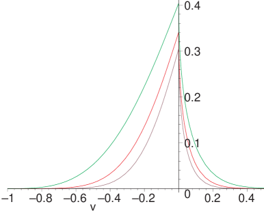
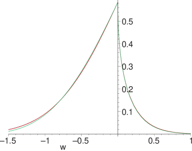
Figure 1: On the left, $\tau_{n}(v)-\tau_{\infty}(v)$ as a function of $v$ for $n=3,5,7$. On the right, the rescaled version $g(w)$ defined in (16).

5 Exact properties of the polynomials characterizing the ground state

In this section we explain how the simple change of variables from $y$ to $\zeta=\sqrt{1+8y^{2}}$ makes obvious a direct relation to polynomials that were studied by Bazhanov and Mangazeev [10, 11, 12], and Razumov and Stroganov [13], in the framework of a particular XYZ chain. They turn out to be related to classical integrable equations and the Painlevé VI transcendent. This relation proves to be very fruitful, because several properties of the our chain can be deduced from already-known features of this XYZ chain. Here we discuss how the polynomials $m_{\pm n}(y^{2})$ characterizing the ground state satisfy a recursion relation in $n$. Like the order parameters discussed above, they are scale free and obey a duality. The scale-free property in particular allows us to find an explicit expression for their $n\to\infty$ behavior.

5.1 XYZ chain and the Painlevé VI tau-function hierarchy

Let us first recall some facts about the particular XYZ chain which possesses some striking properties [17, 10, 11, 12, 13, 5]. The XYZ Hamiltonian is

$$H_{\mathrm{XYZ}}=-\frac{1}{2}\sum_{k=1}^{L}J_{x}\sigma_{k}^{x}\sigma_{k+1}^{x}+J_{y}\sigma_{k}^{y}\sigma_{k+1}^{y}+J_{z}\sigma_{k}^{z}\sigma_{k+1}^{z}\ ,$$ (17)

where the Pauli matrices act on a the two dimensional Hilbert space at each site. As above, we take periodic boundary conditions. The special properties occur along the line of couplings $J_{x}J_{y}+J_{x}J_{z}+J_{y}J_{z}=0$. A convenient parametrization of the coupling constants along this line is given by

$$J_{x}=1+\zeta,\,J_{y}=1-\zeta,\,J_{z}=(\zeta^{2}-1)/2\ .$$ (18)

This model is an off-critical deformation of the XXZ model at $\Delta=J_{z}/J_{x}=-1/2$ (the $\zeta=0$ case). In the conventions of our earlier paper [5], $\zeta=3/s$.

An obvious symmetry of the XYZ spectrum comes by permuting the Pauli matrices. Along the line (18), this results in two useful transformations. A rotation of all spins by $\pi/2$ around the $z$-axis exchangs the $\sigma^{x}\sigma^{x}$- and $\sigma^{y}\sigma^{y}$-terms in $H_{\mathrm{XYZ}}$. This is equivalent to the transformation $\zeta\to-\zeta$. Conversely, rotating all spins by $\pi/2$ around the $y$-axis exchanges the $\sigma^{x}\sigma^{x}$- and $\sigma^{z}\sigma^{z}$-terms. Equivalently this can be done by the homographic transformation

$$\zeta\to\frac{\zeta+3}{\zeta-1},$$ (19)

and rescaling energy by $(\zeta-1)^{2}/4$. Both these transformations are symmetries of the spectrum of $H_{XYZ}$, up to an overall rescaling.

When the number of sites $L$ is odd, all the eigenvalues of $H_{\mathrm{XYZ}}$ are doubly degenerate under spin reversal. As $H_{\mathrm{XYZ}}$ commutes with both the operators $I=\prod_{k=1}^{L}\sigma^{z}_{k}$ and the spin-reversal operator $R=\prod_{k=1}^{L}\sigma^{x}_{k}$ one may decompose the corresponding subspaces into eigenfunctions with $I|\Phi_{\pm}(\zeta)\rangle=\pm|\Phi_{\pm}(\zeta)\rangle$. These are related by spin-reversal $R|\Phi_{\pm}(\zeta)\rangle=|\Phi_{\mp}(\zeta)\rangle$, and thus one may concentrate on one of them, say $|\Phi_{-}(\zeta)\rangle$.

Let us now turn to the ground states of the model. For an odd number of sites $L=2n+1$ the ground states $|\Phi_{\pm}(\zeta)\rangle$ have energy $E_{0}=-L(\zeta^{2}+3)/4$ exactly [17, 7]. Like for our fermion chain, consider a decomposition of the wave function into spin-configuration states $|\Phi_{-}(\zeta)\rangle=\sum_{\alpha}\phi_{\alpha}(\zeta)|\alpha\rangle$. Given that the Hamiltonian itself and the ground state energy are quadratic polynomials in $\zeta$, one can choose the normalization in such a way that all components are polynomials in $\zeta$. An overall constant normalization can be fixed by demanding that the zero-order term for configurations $\tilde{\alpha}=\,\uparrow\uparrow\cdots\uparrow\downarrow\downarrow\cdots\downarrow$ containing a block of $n$ (resp. $n+1$) spins up for $n$ even (resp. odd) equals one. Then it turns out that all polynomials $\phi_{\alpha}(\zeta)$ have integer coefficients and definite parity. Some of them enjoy special properties: the component in front of the fully-polarized state $\,\downarrow\downarrow\cdots\downarrow$ with all spins down is given by

$$\phi_{\downarrow\downarrow\cdots\downarrow}(\zeta)=\zeta^{n(n+1)/2}s_{n}(\zeta^{-2})$$ (20)

where the $s_{n}(z)$ are polynomials in $z$ of degree $\lfloor n^{2}/4\rfloor$ that solve the non-linear recursion relation

$$2z(z-1)(9z-1)^{2}(\ln s_{n}(z))^{\prime\prime}+2(3z-1)^{2}(9z-1)(\ln s_{n}(z))^{\prime}$$

$$+8(2n+1)^{2}\frac{s_{n+1}(z)s_{n-1}(z)}{s_{n}(z)^{2}}-(4(3n+1)(3n+2)+(9z-1)n(5n+3))=0$$ (21)

with initial conditions $s_{0}(z)=s_{1}(z)\equiv 1$. In fact, these are a special case for the Hirota equations for the $\tau$-function hierarchy corresponding to Picard solutions of the Painlevé VI differential equation [18, 19]. Moreover, these polynomials also appear in the computation of the $Q$-function for the ground state of the corresponding eight-vertex model.

There is a number of remarkable properties of the XYZ chain involving the polynomials $s_{n}(z)$; for an extensive list see [12, 13]. As an example let us consider the norm of the wavefunction. Finite-size computations show that it is given in terms of the polynomials $s_{n}(z)$ by

$$||\Phi_{-}(\zeta)||^{2}=(4/3)^{n}\zeta^{n(n+1)}s_{n}(\zeta^{-2})s_{-n-1}(\zeta^{-2}).$$ (22)

Using the invariance of the ground state sector under (19) it is not difficult to show that (22) is invariant under the homographic transformation modulo rescaling by a $\zeta$-dependent function. After a little algebra, one finds the invariant

$$s_{n}(\zeta^{-2})s_{-n-1}(\zeta^{-2})=\left(\frac{3+\zeta}{2\zeta}\right)^{n(n+1)}s_{n}\left(\left(\frac{\zeta-1}{\zeta+3}\right)^{2}\right)s_{-n-1}\left(\left(\frac{\zeta-1}{\zeta+3}\right)^{2}\right).$$ (23)

5.2 The polynomials $m_{\pm n}(y^{2})$ and Painlevé VI

We noted in section 3.3 that $m_{n}(y^{2})$ factorizes into a product of polynomials in $y^{2}$ with integer coefficients when $n$ is odd, and $m_{-n}(y^{2})$ factorizes when $n$ is even. However, as we detail in the appendix, they factorize for all $n$ at the critical point $y=1$. Thus one might hope that they factorize for all $y$ with an appropriate change of variable, and indeed changing to $\zeta$ or $v$ allows this factorization.

This change of variables allows us to find a much more dramatic result: the $m_{\pm n}(y^{2})$ are simply related to the analogous polynomials $s_{n}(z)$ in the XYZ chain! By examining their explicit form up to $n=8$ in terms the new variable $\zeta$, it is readily apparent that they are related to the $s_{n}(z)$ by the following equations:

$$m_{n}\left(y^{2}=(\zeta^{2}-1)/8\right) = \ \frac{\zeta^{\lfloor(n-1)^{2}/2\rfloor}}{2^{(n-1)(n-2)/2}}\frac{s_{n-1}(\zeta^{-2})}{s_{n-1}(0)},$$ (24)

$$m_{-n}\left(y^{2}=(\zeta^{2}-1)/8\right) = \ \frac{\zeta^{\lfloor n^{2}/2\rfloor}}{2^{(n-1)(n+2)/2}}\frac{s_{-n}(\zeta^{-2})}{s_{-n}(0)}.$$ (25)

with $s_{n}(0)=1$ for $n\geq 0$, and $s_{n}(0)=(3/4)^{-n-1}$ for $n<0$.

The most important consequence of this identification is that the polynomials $m_{\pm n}(y^{2})$ can be obtained from a recursion relation. Moreover, the ground states in the fermion and XYZ chains have analogous special properties: for example, (20) is analogous to (8).

We can use the knowledge about properties of the $s_{n}(z)$ in order to obtain ground state properties of our fermion chain. When the transformation (19) is rewritten in terms of $v=(3-\zeta)/(\zeta+1)$, this is precisely the $v\to-v$ duality discussed in section (4.2). The square norm of the ground state wavefunctions of the fermion chain, given in (7), are quite similar, although not identical to (22). However considering the combination of (7), (24) and (25), it is a straightforward consequence of (23) that the product of the ground state square norms $N_{n}(v)=||\Psi^{\rm e}(y)||^{2}||\Psi^{\rm o}(y)||^{2}$ has the following invariance property

$$N_{n}\left(-v\right)=\left(\frac{v+1}{2}\right)^{n(n+1)}N_{n}(v).$$ (26)

Given this invariance property it is not surprising that all quantities studied in section 4.2 with nice duality properties involve both parity sectors.

5.3 Scale-free properties

Knowing that the $m_{\pm m}(y^{2})$ are related to the Painlevé VI equation teaches us a great deal about the ground states of our fermion model. Here we show how the lessons we have learned in the analysis of the fermion model give new insight into the polynomials $s_{n}(x)$. In particular, we show how they obey the scale-free property discussed in [5] and above in section 4.2. Combining this with the Hirota equations (21) allows us to derive the scale-free coefficients explicitly. We can then sum this series by approximating the Hirota equation, and so find an asymptotic expression for the $s_{n}$ themselves.

To this end, let us introduce another reparametrization $x=(1-\zeta)/(3+\zeta)$. Then define a rescaled version of $s_{n}$ via

$$S_{n}(x)=s_{n}\left(1/\zeta^{2}\right)(1+x)^{\frac{n(n+1)}{2}}(1-x)^{\frac{n(n+2)}{2}}(1+3x)^{\frac{n^{2}}{2}}/s_{n}(1)\ .$$ (27)

where $s_{n}(1)=2^{n(n-1)/2}$ for $n\geq 0$, and $s_{n}(1)=3^{-n-1}2^{(n+2)(n+1)/2}$ for $n<0$. The Taylor series expansion of $S_{n}(x)$ around the trivially solvable point $x=0$ is scale free: for $n>0$ the first $n$ terms in this expansion are independent of $n$, while for $n<0$ the first $-n-1$ terms in this expansion are independent of $n$. The scale-free part of the expansion is

$$S(x)=1+x+2x^{3}-x^{4}+9x^{5}-6x^{6}+54x^{7}-36x^{8}+\dots$$

We can determine all the coefficients and a summed form directly from (21): the $S_{n}(x)$’s are solution to the recurrence equation

$$p(x)(\ln S_{n}(x))^{\prime\prime} +q(x)(\ln S_{n}(x))^{\prime}+2(2n+1)^{2}\left(\frac{S_{n+1}(x)S_{n-1}(x)}{S_{n}(x)^{2}}-1\right)=r(x),$$

with the coefficients

$$p(x) =\frac{2x(x-1)(x+1)^{2}(3x-1)^{2}}{1+3x},$$

$$q(x) =\frac{(x+1)(3x-1)(1+8x-22x^{2}+45x^{4})}{(1+3x)^{2}},$$

$$r(x) =-3x^{3}-x^{2}+3x-1.$$

Let us now make the assumption that the limit $S_{\infty}(x)=\lim_{n\to\infty}S_{n}(x)$ exists and that we can neglect the term $\propto(2n+1)^{2}$ (i.e. the ratio $S_{n+1}(x)S_{n-1}(x)/S_{n}(x)^{2}-1$ decays faster than $1/n^{2}$, at least for small $x$). Thus we must solve the differential equation

$$p(x)(\ln S_{\infty}(x))^{\prime\prime}+q(x)(\ln S_{\infty}(x))^{\prime}=r(x)$$ (28)

with initial conditions $S_{\infty}(x=0)=1,\,S_{\infty}^{\prime}(x=0)=1$. The unique solution is given by the simple function

$$S_{\infty}(x)=\frac{(1+3x)^{5/24}}{(1-x)^{3/8}(1+x)^{1/8}(1-3x)^{1/24}}$$ (29)

which indeed generates all the scale-free coefficients.

An illustration of this function compared to $S_{n}(x)$ with $n=\pm 50$ is given in figure 2(a). The recurrence relation allows us to compute the first corrections to the scale-free form as well. We have $S_{n}(x)/S_{\infty}(x)=1+b_{n}x^{n+1}+c_{n}x^{n+2}+\dots$ Upon inserting this into the equation for $S_{n}(x)$, and expanding around $x=0$ we find the recursion relations $(n+1)b_{n}=2(2n+1)b_{n-1},\,b_{0}=-1$ and $(n+2)(2n+3)c_{n}-2(2n+1)^{2}c_{n-1}-4b_{n}=0,\,d_{0}=1/2$ which are readily solved:

$$b_{n}=-\frac{1}{2}\left(\begin{array}[]{c}2n+2\\ n+1\end{array}\right),\quad c_{n}=\frac{1}{n+2}\left(\begin{array}[]{c}2n+2\\ n+2\end{array}\right).$$ (30)

Hence the first correction is a binomial – a quite common feature that we observed for other quantities as well.

The preceding procedure relied on an expansion around the trivially solvable point $x=0$. As we did with the order parameters, we can also understand the scaling around the critical point $x=1/3$. From the asymptotic formula (29), we see that $S_{\infty}(x)$ displays a power-law singularity with exponent $-1/24$. Conversely, for finite $n$ we find at this point that

$$\frac{S_{n+1}(1/3)}{S_{n}(1/3)}=\frac{2^{4(n+1)}s_{n+1}(1/9)s_{n}(1)}{3^{2n+5/2}s_{n}(1/9)s_{n+1}(1)}=\frac{2^{4n+3}}{3^{3n+5/2}}\frac{n!(3n+2)!}{((2n+1)!)^{2}}$$ (31)

The value $s_{n}(1/9)$ necessary here can directly be inferred from the Hirota equations by setting $z=1/9$. Upon application of Stirling’s formula for large $n$, it is not difficult to derive from this expression the asymptotic behavior $S_{n}(x=1/3)\sim n^{1/36}$ for large positive $n$. For large negative $n$ the scaling is identical because of $S_{-n-1}(1/3)=\sqrt{3}S_{n}(1/3)$. Thus to obtain something finite in the $n\to\infty$ we obtain again the result from section 4.3 that near the critical point, the deformation parameter (here $x-1/3$) must be rescaled by a power of $n^{2/3}$. In the context of differential equations, such a relation between properties in the two limits is known as a “connection formula”. The rescaled functions $\sigma_{n}(t)=n^{-1/36}S_{n}(1/3-n^{-2/3}t)$ are illustrated in figure 2(b). As before, we observe a remarkable collapse for large $n$, this time however without subtraction of any infinite-volume term like $n^{-1/36}S_{\infty}(1/3-n^{-2/3}t)$. It would be very interesting to find the scaling functions $\sigma_{\pm}(t)=\lim_{n\to\pm\infty}\sigma_{n}(t)$. A detailed analysis of the Hirota equations [23] yields at least the first two Taylor coefficients

$$\sigma_{\pm}(t)=C_{\pm}\left(1\pm\frac{3\Gamma(2/3)}{4\Gamma(4/3)}t+O(t^{2})\right),$$ (32)

where $C_{+}={G(3/2)^{2}}/({G(4/3)G(5/3)})=1.013993\dots$ and $C_{-}=\sqrt{3}C_{+}$. Here $G(z)$ denotes the Barnes $G$-function, defined through the functional equation $G(z+1)=\Gamma(z)G(z)$.

(a)		(b)

Figure 2: (a) $S_{n}(x)$ for $n=50$ (dotted line) and $n=-50$ (dashed line) together with the generating function $S_{\infty}(x)$. (b) Near the critical point $x=1/3$ the rescaled functions $\sigma_{n}(t)$ collapse for large $n$: here we show $n=10,20,\dots,50$. A similar behavior can be observed for negative $n$.

6 Conclusion

We have studied an off-critical staggered model for supersymmetric lattice fermions with hard-core exclusion, and found some striking properties of its ground state. We showed how the supersymmetry allows the entire ground state to be characterized by a single polynomial, and related this to solutions of the Hirota equations, which earlier arose in an XYZ chain in the same universality class. We saw how a variety of special properties allowed the determination of exact expressions for the order parameters and critical exponents.

The precise connection between the supersymmetric fermion model and the XYZ chain is surprising for several reasons. First, it is known that the critical point of the fermion chain can be transformed to the XXZ chain at $\Delta=-1/2$ with twisted boundary conditions and an even number of sites [4, 9]. Even though there is a relation between the cases $L=2n$ with twisted boundary conditions and $L=2n+1$ with periodic boundary conditions for this XXZ chain [20], what happens off criticality remains mysterious. In particular, no XYZ chain with twisted boundary conditions that remains integrable is known, since there it has no obvious $U(1)$ conservation law. Note, however, the fermion chain does possess a $U(1)$ fermion number conservation law. Another distinction between the two is in the dualities. For the XYZ chain, the duality transformation (19) is related to simple unitary transformations on the Hilbert space (spin rotations) and obvious invariance properties of the corresponding Hamiltonian. In the fermion case however, the transformation on the coupling constant $y$ is highly non-linear, and a realization of the duality on the Hilbert space through a unitary transformation seems to be less evident.

These observations give a strong hint that there remains much structure to be uncovered in both the fermion and XYZ chains. As the latter are related to the eight-vertex model at the special crossing parameter $\eta=\pi/3$, powerful theoretical tools such as Baxter’s famous TQ-equation can be used for their analysis. For example, it allows the exact evaluation of the nearest-neighbor spin correlators in finite size [23]. In the case of the fermion chain, similar relations remain to be discovered.

Appendix A Combinatorial properties at the critical point

Given the connection between the critical model and the XXZ chain at $\Delta=-1/2$, it is natural to expect that the values $m^{\pm}_{n}(y=1)$ are related to combinatorial numbers enumerating alternating sign matrices and related objects. By explicitly finding the ground states at $y=1$, some of these combinatorial properties were explored in [16]. Here we analyze the particular case of $N=3n$ and periodic boundary conditions in more depth.

First, we notice that at $y=1$ we find

$$m_{-2k}(1)=3m_{2k}(1)\quad\mbox{and}\quad m_{1-2k}(1)=m_{2k-1}(1),$$

for $k=1,2,\dots$. Therefore it will be sufficient to concentrate on the parity-even sequence $m_{n}(1)$. For odd $n=2k-1$ we thus find $m_{2k-1}(1)=1,5,198,63206,163170556,\dots$ This sequence corresponds to the numbers $A_{UU}(4k)$ of $4k\times 4k$ alternating sign matrices of type UU [21]. It is known to factorize into

$$m_{2k-1}(1)=A_{UU}(4k)=A_{V}(2k+1)\times A_{UU}(4k;1,1,1)$$ (33)

where

$$A_{V}(2k+1) =\frac{1}{2^{k}}\prod_{j=1}^{k}\frac{(6j-2)!(2j-1)!}{(4j-1)!(4j-2)!},$$

$$A_{UU}(4k;1,1,1) =(-3)^{k^{2}}2^{2k}\prod_{i=1}^{2k}\prod_{{j=1,2\mid j}}^{2k+1}\frac{3j-3i+2}{j-i+2n+1}.$$

Here $A_{V}(2k+1)$ is the number of alternating sign $(2k+1)\times(2k+1)$ matrices symmetric about the vertical axis, also the number of $(2k)\times(2k)$ off-diagonally symmetric alternating sign matrices, and $A_{UU}(4k;1,1,1)$ expansion coefficients of a generating function appearing in [21, 22].

For even $n=2k$ we find the values $m_{2k}(1)=1,14,1573,1427660,\dots$ As is the case of an odd number of particles, this sequence can be factorized according to

$$m_{2k}(y=1)=N_{8}(k)\times\frac{A(2k-1)}{A_{V}(2k-1)},\quad k=1,2,\dots$$ (34)

with the numbers of cyclically symmetric transpose complementary plane partitions $N_{8}(k)$ given by [8]

$$N_{8}(k)=\prod_{j=0}^{k-1}(3j+1)\frac{(6j)!(2j)!}{(4j)!(4j+1)!},$$

and the well-known numbers of $n\times n$ alternating sign matrices

$$A(k)=\prod_{j=0}^{k-1}\frac{(3j+1)!}{(k+j)!}.$$

We emphasized the factorizations because it turns out that the subfactors of $m_{2k-1}(y^{2})$ and $m_{-2k}(y^{2})$ are in one-to-one correspondence with the factors in (33) and (34) when setting $y=1$.

References

References

- [1] R.J. Baxter, Exactly Solved Models in Statistical Mechanics (Academic, London, 1982)
- [2] E. Witten, Constraints on supersymmetry breaking, Nucl. Phys. B 202 (1982) 253
- [3] P. Fendley, K. Schoutens and J. de Boer, Lattice Models with N=2 Supersymmetry, Phys. Rev. Lett. 90 (2003) 120402, arXiv:hep-th/0210161.
- [4] P. Fendley, B. Nienhuis and K. Schoutens, Lattice fermion models with supersymmetry, J. Phys. A: Math. Gen. 36 (2003) 12399, arXiv:cond-mat/0307338.
- [5] P. Fendley and C. Hagendorf, Exact and simple results for the XYZ and strongly interacting fermion chains, J. Phys. A: Math. Theor. 43 (2010) 402004
- [6] A. V. Razumov and Y. G. Stroganov, Spin chains and combinatorics: twisted boundary conditions, J. Phys. A: Math. Gen. 34 (2001) 5335, arXiv:cond-mat/0102247.
- [7] Y. Stroganov, The 8-vertex model with a special value of the crossing parameter and the related xyz chain, in Integrable structures of exactly solvable two-dimensional models of quantum field theory (Kiev 2000), Volume 35 of NATO Sci. Ser. II Math. Phys. Chem., pages 315–319, Kluwer Acad. Publ., Dordrecht, 2001.
- [8] J. de Gier, M. T. Batchelor, B. Nienhuis and S. Mitra, The XXZ spin chain at : Bethe roots, symmetric functions, and determinants, J. Math. Phys. 43 (2002) 4135, arXiv:math-ph/0110011.
- [9] X. Yang and P. Fendley, Non-local space-time supersymmetry on the lattice, J. Phys. A 37 (2004) 8937, arXiv:cond-mat/0404682.
- [10] V. V. Bazhanov and V. V. Mangazeev, Eight-vertex model and non-stationary Lamé equation, J. Phys. A: Math. Gen. 38 (2005) L145,
- [11] V. V. Bazhanov and V. V. Mangazeev, The eight-vertex model and Painlevé VI, J. Phys. A: Math. Gen. 39 (2006) 12235, arXiv:hep-th/0602122.
- [12] V. V. Mangazeev and V. V. Bazhanov, The eight-vertex model and Painlevé VI equation II: eigenvector results, J. Phys. A: Math. Theor. 43 (2010) 085206, arXiv:0912.2163.
- [13] A. V. Razumov and Y. G. Stroganov, A possible combinatorial point for the XYZ spin chain, Theor. Math. Phys. 164 (2010) 977, 0911.5030.
- [14] L. Huijse, University of Amsterdam thesis (2010)
- [15] P. Fendley and K. Intriligator, Scattering and Thermodynamics of Fractionally-Charged Supersymmetric Solitons, Nucl. Phys. B 372, 533 (1992), arXiv:hep-th/9111014
- [16] M. Beccaria and G.F. De Angelis, Exact Ground State and Finite Size Scaling in a Supersymmetric Lattice Model,” Phys. Rev. Lett. 94, 100401 (2005), arXiv:cond-mat/0407752.
- [17] R.J. Baxter, Solving models in statistical mechanics, Adv. Stud. Pure Math. 19 (1989) 95,
- [18] K. Okamoto, Studies on the Painlevé equations. I: Sixth Painlevé equation PVI, Annali di Matematica pura ed applicata 146 (1987) 337.
- [19] V. V. Mangazeev, Picard solution of Painlevé VI and related tau-functions, arXiv:1002.2327 2010.
- [20] P. Di Francesco, P. Zinn-Justin and J.-B. Zuber, Sum rules for the ground states of the O(1) loop model on a cylinder and the XXZ spin chain, J. Stat. Mech. 8 (2006) 11, arXiv:math-ph/0603009.
- [21] G. Kuperberg, Symmetry Classes of Alternating-Sign Matrices under One Roof, Ann. Math. 156 (2002) 835, arXiv:math/0008184
- [22] D. P. Robbins, Symmetry Classes of Alternating Sign Matrices, arXiv:math.CO/0008045.
- [23] C. Hagendorf, in preparation (2010).