Partially Cooled Shocks: Detectable Precursors in the Warm/Hot Intergalactic Medium

Abstract

I present computations of the integrated column densities produced in the post-shock cooling layers and in the radiative precursors of partially-cooled fast shocks as a function of the shock age. The results are applicable to the shock-heated warm/hot intergalactic medium which is expected to be a major baryonic reservoir, and contain a large fraction of the so-called ”missing baryons”. My computations indicate that readily observable amounts of intermediate and high ions, such as C IV, N V, and O VI are created in the precursors of young shocks, for which the shocked gas remains hot and difficult to observe. I suggest that such precursors may provide a way to identify and estimate the ”missing” baryonic mass associated with the shocks. The absorption-line signatures predicted here may be used to construct ion-ratio diagrams, which will serve as diagnostics for the photoionized gas in the precursors. In my numerical models, the time-evolution of the shock structure, self-radiation, and associated metal-ion column densities are computed by a series of quasi-static models, each appropriate for a different shock age. The shock code used in this work calculates the nonequilibrium ionization and cooling, follows the radiative transfer of the shock self-radiation through the post-shock cooling layers, takes into account the resulting photoionization and heating rates, follows the dynamics of the cooling gas, and self-consistently computes the photoionization states in the precursor gas. I present a complete set of the age-dependent post-shock and precursor columns for all ionization states of the elements H, He, C, N, O, Ne, Mg, Si, S, and Fe, as functions of the shock velocity, gas metallicity, and magnetic field. I present my numerical results in convenient online tables.

1. Introduction

It is a remarkable fact the in the present day universe about a half of the baryonic matter is ”missing”, in that it has not yet been accounted for observationally. Hydrodynamic simulations of structure formation suggest that these baryons may reside in a ”warm-hot intergalactic medium” (WHIM), with temperatures in the range $10^{5}-10^{7}$ K (e.g. Cen & Ostriker 1999; Davé et al. 2001; Bertone et al. 2008). The WHIM is produced by the shock waves that occur as gas falls from the diffuse intergalactic medium into the dense regions where galaxies form, and is expected to remain hot because of the low densities and high temperatures involved.

Recent observations have confirmed the existence of a hot, $10^{5}-10^{7}$ K gas, both in the local Universe (e.g. Fang et al. 2006), and in more distant environments (e.g. Tripp et al. 2007; Savage et al. 2005; Buote et al. 2009; Narayanan et al. 2009; Fang et al. 2010; Danforth et al. 2010). Important ions for its detection include O VI, O VII, O VIII, Ne VIII, and Ne IX (see also Bertone et al. 2010a, 2010b; Ursino et al. 2010). In some cases, lower ionization species are also associated with the warm/hot gas. For example, Savage et al. (2005) and Narayanan et al. (2009) reported on absorption-line systems at a redshift of $\sim 0.2-0.3$, containing C III, O III, O IV, O VI, N III, Si III, Si IV, and Ne VIII. They invoked an equilibrium two-phase model, in which most of the ions are created in a warm ($\sim 2\times 10^{4}$ K) photoionized cloud, while O VI and Ne VIII are created in a hotter ($\sim 5\times 10^{5}$ K), collisional phase. The inferred temperature for the collisional phase is within the range of temperatures where departures from equilibrium ionization are expected to take place (e.g. Gnat & Sternberg 2007). While observations have confirmed the existence of warm/hot clouds, it remains to be determined what fraction of baryons they harbor, and whether they confirm the theoretical predictions regarding the shock heated WHIM (Furlanetto et al. 2005).

In Gnat & Sternberg (2009; hereafter GS09) we computed the metal-absorption column densities in steady-state fast radiative shocks. We estimated the metal-ion column densities in the post-shock cooling layers, under the assumption of steady-state, completely-cooled shocks (e.g. Cox 1972; Dopita 1976, 1977; Raymond 1979; Shull & McKee 1979; Daltabuit, MacAlpine & Cox 1978; Binette et al. 1985; Shapiro & Kang 1992; Dopita & Sutherland 1995, 1996; Allen et al. 2008). The steady-state assumption is only valid for shocks that exist over a time-scale that is longer than their cooling times. In younger shocks that have not yet cooled completely, the shock structure, self-radiation, and resulting column densities are time-dependent. For the cosmological shocks that produce the WHIM, the steady-state assumption is often not valid.

In this paper, I reexamine the absorption-line signatures of fast astrophysical shock, but relax the assumption that they are fully-cooled and in steady-state. I explicitly consider the properties of partially cooled shocks as a function of shock age. I compute the integrated column densities produced in the post-shock cooling layers and in the radiative precursors of such partially-cooled fast shocks. The time-evolution of the shock structure, self-radiation, and associated metal-ion column densities are evaluated by a series of quasi-static models, each appropriate for a different shock age.

I use the shock code presented in GS09 that computes the nonequilibrium ionization and cooling, follows the radiative transfer of the shock self-radiation through the post-shock cooling layers, takes into account the resulting photoionization and heating rates, follows the one-dimensional dynamics of the cooling gas, and self-consistently computes the photoionization states in the precursor gas.

As in GS09, I focus on fast shocks, with velocities of $600$ and $2000$ km s^-1, corresponding to initial temperatures of $5\times 10^{6}$ and $5\times 10^{7}$ K, and I present a complete set of results for metallicities $Z$ ranging from $10^{-3}$ to twice the solar abundance of heavy elements. Investigating how the absorption line signatures of fast astrophysical shocks depend on metallicity is particularly interesting in the context of the WHIM, as parts of the WHIM are expected to have significant subsolar metallicities (e.g. Cen & Ostriker 2006).

I consider shocks in which the magnetic field is negligible ($B=0$) so that cooling occurs at approximately constant pressure, and shocks in which the magnetic-pressure dominates the pressures everywhere ($B/\sqrt{\rho}\gg v_{s}$), and the density remains constant.

In the computations presented here I use the same simplifying assumptions made in GS09. First, I neglect any thermal instabilities that may form in the post-shock cooling layers, even though such instabilities are known to occur for shock velocities in excess of $140$ km s^-1. Second, I assume that the electron and ion temperatures are equal in the downstream gas, because the electron-ion equipartition times are typically $<1\%$ of the cooling time (GS09). This may lead to some errors for very young shocks that exist for shorter time-scales. Third, I assume that the shocked material is dust-free, or that any initial dust penetrating the shock is rapidly destroyed (e.g. by thermal sputtering) on a time scale that is much shorter than the cooling time. For a detailed discussion of these assumptions see Section 1 in GS09.

In addition to the assumptions of GS09, I make one further assumption when following the time-dependent evolution of the shock structure. I assume that the shock evolution is quasi-static, so that it can be approximated by a series of “self-contained” models for the different ages, which are independent of each other. Since the shock structure, self-radiation and associated precursor ionization states do, in fact, evolve continuously over the lifetime of the shock, this discretizaton does lead to small errors in the computed structure of young shocks. However, as I demonstrate in the following sections, once the shocks exist for $\gtrsim 1\%$ of their cooling times, this approximation is generally valid. In addition, the quasi-static approximation does not significantly affect the computed self-radiation or the integrated column densities.

Therefore, the results for very early times (young shocks with ages $<1\%$ of the shock cooling time) suffer from two main limitations, namely the uncertain validity of the quasi-static assumption, and an age comparable to the electron-ion equipartition time. In addition, at least in the cosmological context, it is not very likely that we will observe systems with lifetimes that are considerably shorter than a Hubble time. However, for the sake of completeness, and because the integrated metal-ion column densities are not very sensitive to these assumptions, I include young shocks in the discussion that follows.

The outline of this paper is as follows. In Section 2, I describe the physical processes that I consider in my computations. These include the ionization, dynamics, cooling and heating, radiative transfer, and the treatment of the initial ionization states in the gas approaching the shock front. In Section 3, I discuss the shock structure and emitted radiation, and investigate how they depend on the shock age, as a function of the controlling parameters, including the gas metallicity, shock velocity, and magnetic field. In Section 4, I investigate how the integrated post-shock column densities evolve as a function of shock age. I describe the full set of post-shock and precursor column densities versus age in Sections 5 and 6, respectively. I explain how the UV absorption line signatures of the radiative precursors may dominate those produced in the downstream gas over a significant fraction of the shock lifetime, and may thus serve as means for identifying and detecting young fast shocks. In Section 7, I demonstrate how ion-ratio diagrams may serve as diagnostics for gas in the radiative precursors of partially-cooled fast astrophysical shocks. The detection and identification of precursor gas may allow us to confirm the existence of the hot, unobservable, shocked counterpart, and to infer its associated baryonic content. I summarize in Section 8, and conclude in 9.

2. Ionization, Cooling, Dynamics, and Radiative Transfer

In this section I describe the physical processes that I take into account in the shock models, including the ionization, dynamics, cooling and heating, radiative transfer, and the treatment of the initial ionization states in the gas approaching the shock front. I also describe the method used to follow the evolution of the shock structure and properties.

After passing the shock front, the gas is initially heated to the shock temperature $T_{s}\gtrsim 10^{6}$ K, and then cools and recombines, to a degree determined by the shock age. I follow a gas element as it advances through the post-shock flow. As in GS09, if the gas cools faster than it recombines, nonequilibrium ionization becomes significant, and may affect the cooling rate of the gas. I follow the coupled evolution of the ionization states and cooling efficiencies.

In this work, I use and improve the shock code developed in GS09. This code calculates the nonequilibrium ionization and cooling, follows the radiative transfer of the shock self-radiation through the post-shock cooling layers, takes into account the resulting photoionization and heating rates, follows the dynamics of the cooling gas, and self-consistently computes the initial ionization states of the precursor gas.

For the ionization, I consider all ionization states of the elements H, He, C, N, O, Ne, Mg, Si, S, and Fe. I include collisional ionization by thermal electrons, photoionization, Auger ionization, radiative recombination, dielectronic recombination, and neutralization and ionization by charge transfer reaction with hydrogen and helium atoms and ions (GS07, GS09, and references therein). I follow the time-dependent ionization equation for each ion individually (see equation 1 in GS09). I assume the elemental abundances reported by Asplund et al. (2005) for the photosphere of the Sun, and the enhanced Ne abundance recommended by Drake & Testa (2005). I list these abundances in Table 1. I also assume a primordial helium abundance $A_{\rm He}=1/12$ (Ballantyne et al. 2000), independent of Z.

Table 1Solar Elemental Abundances

Element	Abundance
	(X/H)⊙
Carbon	$2.45\times 10^{-4}$
Nitrogen	$6.03\times 10^{-5}$
Oxygen	$4.57\times 10^{-4}$
Neon	$1.95\times 10^{-4}$
Magnesium	$3.39\times 10^{-5}$
Silicon	$3.24\times 10^{-5}$
Sulfur	$1.38\times 10^{-5}$
Iron	$2.82\times 10^{-5}$

For the cooling, I follow the electron cooling efficiency, $\Lambda(T,x_{i},Z)$ (erg s^-1 cm³), which depends on the gas temperature, ion fractions, and abundance of heavy elements. This includes the removal of electron kinetic energy via collisional excitation followed by prompt line emission, thermal bremsstrahlung, recombination with ions, and collisional ionizations (see GS07; based on the cooling functions included in Cloudy ver. 07.02.00, Ferland et al. 1998). I also follow the heating rate $\Gamma(x_{i},Z,J_{\nu})$ (erg s^-1), due to the absorption of the shock self-radiation $J_{\nu}$, by gas further downstream. The net local cooling rate is given by $n_{e}n_{\rm H}\Lambda-n\Gamma$, where $n$ is the total gas particle density.

For the dynamics, I assume one-dimensional strong shocks, and neglect any thermal instabilities that may form. I follow the standard Rankine-Hugoniot conditions (see equations 3 in GS09), which represent the conservation of mass, momentum, and energy fluxes in the flow. The assumption of a strong shock implies the familiar jump conditions (e.g. Draine & McKee 1993) which relate the pre-shock, and post-shock physical properties: $n_{0}=4n_{\rm pre}$, and $v_{0}=1/4\;v_{s}$, where $n_{0}$ and $v_{0}$ are the post-shock particle density and velocity, $n_{\rm pre}$ is the pre-shock density, and $v_{s}$ is the shock velocity.

I use the Rankine-Hugoniot conditions to follow the evolution of the gas pressure, density and velocity along the flow. As in GS09, I consider two limiting cases. First, I consider flows in which $B=0$ everywhere. Second, I consider shocks in the which magnetic field is dynamically dominant, with $B/\sqrt{\rho}\gg v_{s}$, so that it dominates the pressure throughout the flow.

When $B=0$ everywhere, the gas cools at an approximately constant pressure, and the final pressure far downstream is $P_{\infty}=4/3\;P_{0}$, where $P_{0}$ is the pressure immediately post-shock (see Section 2.3 in GS09 for details). In the limit of strong magnetic field ($B/\sqrt{\rho}\gg v_{s}$), the Rankine-Hugoniot conditions imply constant density and velocity throughout the flow, so that $\rho=\rho_{0}$, and $v=v_{0}$ everywhere.

To evaluate the intensity of the radiation along the flow, I follow the radiative transfer equation. As in GS09, I use a Gaussian quadrature scheme (Chandrasekhar 1960) to evaluate the local intensity of radiation as a function of distance from the shock front. I follow the specific intensity $I_{\nu}(\mu)$ along $10$ downstream directions between $\mu=1$ (parallel to the shock velocity) and $\mu=0$. The flow is divided into thin slabs. In each slab I use Cloudy to evaluate the local absorption ($\alpha_{\nu}$) and emission ($\epsilon_{\nu}$) coefficients appropriate for the local conditions. The radiation transfer equation can then be followed along the $10$ values of $\mu$, to calculate the input intensities for the next slab. Finally the mean intensity, $J\nu=\frac{1}{4\pi}\int I_{\nu}(\mu)d\Omega$, is computed locally and used in evaluating the local heating and photoionization rates.

The shock self-radiation also determines the ionization states in the radiative precursor, which in turn, affects the initial evolution of the post-shock gas. For shock velocities in excess of $175$ km s^-1 such as I consider here, a stable radiative precursor will form (GS09; Dopita & Sutherland 1996).

In GS09, we allowed the shock to evolve until the gas cooled down to a temperature $T_{\rm low}=1000$ K, at which we terminated the computation. In this work, I construct shock models as a function of the final shock age. The shock code used in this work does not produce truly time-evolving computations. Instead, the evolution of the shock properties with age is approximated by a series of quasi-steady-state models, each assumed to be independent of other ages as described below. For each age, I terminate the computation once a Lagrangian gas element starting at the shock front exists for a duration that equals the desired age. The shock structure, self-radiation, and the resulting precursor ionization, are then functions of this age. For each combination of shock parameters (temperature, metallicity, and magnetic field) I construct a series of such “stand-alone” self-consistent models for a range of ages.

To self-consistently calculate the coupled ionization states in the precursor and the post-shock structure, iterations are required. In the first iteration, I assume that the gas starts in collisional ionization equilibrium (CIE) at the shock temperature. I then compute the resulting shock model, ending at the appropriate shock age, while following the radiative transfer in the downstream direction.

At early times, the shocks remain optically thin throughout. In this case, I assume that the flux at the termination point, $F_{\nu}(l_{\rm age})$ equals the flux entering the radiative precursor. I use $F_{\nu}(l_{\rm age})$ to compute the ionization states of the gas entering the shock. For older shocks, the gas becomes thick to its own self-radiation at some large distance from the shock front $l_{\rm thick}$. In this case, I assume that the flux which ionizes the precursor equals $F_{\nu}(l_{\rm thick})$. In both cases I use the photoionization code Cloudy (ver. 07.02.00) to compute the equilibrium photoionization states in the steady precursor. These ionization states are the initial conditions for the next iteration. This process is repeated until the shock self-radiation and resulting initial ionization states converge. The assumption that the upstream radiation field equals $F_{\nu}(l_{\rm thick})$ (or $F_{\nu}(l_{\rm age})$) is based on the fact that the post-shock gas is optically thin in this region. Nevertheless, geometrical effects as well as scatterings in the downstream gas, may increase the intensity of the radiation in upstream directions. This assumption may thus lead to some underestimate of the intensity of radiation photoionizing the precursor.

In GS09, we found that two iteration were sufficient to ensure the convergence of the complete (steady-state) shock models. However, for the younger partial shocks considered here, I find that more iterations are often required to obtain a self-consistent solution. The numerical scheme used here is identical to the one described in GS09 (Section 2.6), with the exception of the different termination criterion. To ensure the convergence of the different models, I have implemented an algorithm that automatically checks for convergence and initiates the next iteration if necessary. I found that between $2$ and $19$ iterations are required, depending on the shock parameters and age.

The approximation used here, where the time-dependent structure of the shock is approximated by a series of quasi-static, “self-contained” models, introduces some inaccuracies. Since the shock structure, self-radiation and associated precursor ionization states do, in fact, evolve continuously over the lifetime of the shock, the discretizaton may lead to some error in the resulting structure of young shocks. However, as I demonstrate below, once the shocks exist for $\gtrsim 1\%$ of their cooling times, the approximation is generally valid. In addition, this approximation does not significantly affect the computed self-radiation or resulting integrated column densities.

In the discussion that follows, all ages and times are presented in terms of $n_{0}\times t$, the post-shock hydrogen density times time. This scheme makes the results nearly independent of density (but see Section 3.5 in GS09).

3. Shock Structure, Ionization & Cooling

In this section, I describe the shock structure, and focus on how it depends on the shock age. I consider two values of shock temperature: $5\times 10^{6}$ K ($v_{s}\simeq 600$ km s^-1) and $5\times 10^{7}$ K ($v_{s}\simeq 1920$ km s^-1), and five different values of the metallicity $Z$, from $10^{-3}$ to $2$ times the metal abundance of the Sun. For each shock temperature and gas metallicity I study shocks in the $B=0$ and strong-$B$ limits.

3.1. A strong-$B$ (isochoric), $T_{s}=5\times 10^{6}$ K, solar metallicity Shock

To illustrate the behavior of the post-shock cooling gas, I first focus on the results for a strong-$B$ shock with $T_{s}=5\times 10^{6}$ K, and $Z=1$. Figure 1 shows the temperature profile of the post-shock cooling layers for the complete shock. The crosses along the curve show the times for which partial shock models were computed.

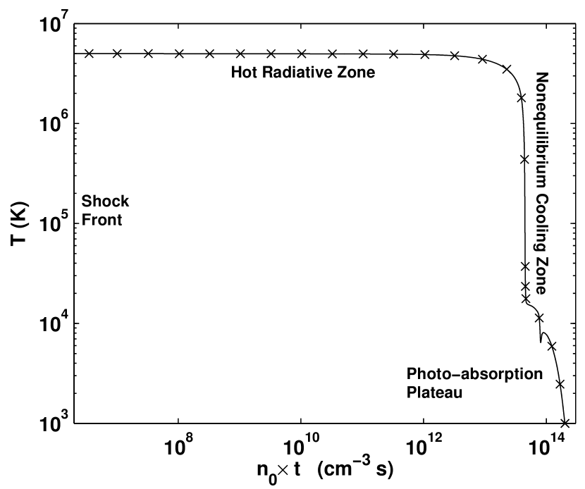
Figure 1.— Complete shock structure for $T=5\times 10^{6}~{}K$, $Z=1$ solar in the strong$-B$ limit. The crosses mark the final ages for which partial shock models where computed.

The complete shock (Figure 1) is composed of several zones (GS09). The photoionized precursor is heated to the shock temperatures after passing the shock front. It enters a “hot radiative” zone in which cooling is slow. It later passes through the “nonequilibrium cooling” zone, in which cooling is rapid, and departures from equilibrium ionization may occur. After the neutral ion fraction rises, photoabsorption heating becomes efficient, and the gas enters a “photoabsorption plateau”, during which the temperature declines more slowly. Finally, after a cooling time, the gas cool completely.

This picture is modified for time-dependent shocks that exist over a time-scale shorter than their cooling time. I now consider how the shock structure, self-radiation, and precursor ionization depend on the shock age.

The initial ionization states of the gas that enters the shock are set by photoionization equilibrium of the precursor gas with the shock self-radiation. This radiation field builds up as the shock forms. Initially, a young shock emits faint radiation, and the precursor gas remains largely neutral. As time passes, the shock self-radiation builds up until the final complete radiation field is obtained after a cooling time. Even then, the photoionization equilibrium temperature in the radiative precursor is significantly lower than the shock temperature, and the gas remains underionized compared to CIE at $T_{s}$.

Figure 2 shows the radiation flux emitted by a $5\times 10^{6}$ K, solar metallicity shock at various ages. Some age-labels are indicated near the spectra for guidance. Initially, the precursor gas is almost entirely neutral, making electron impact excitations and thermal bremsstrahlung emission inefficient. The three bottom curves in Figure 2 show this initial stage, for which the precursor electron fraction is small ($n_{0}t<10^{8}$ cm^-3 s).

After the radiation flux builds up as the shock develops, the ionized fraction in the precursor becomes significant. The various cooling and emission processes are then much more efficient, and the radiation field rises considerably. The radiation field continues to grow with shock age, because the depth of the emitting region increase with time ($10^{8}<n_{0}t<3\times 10^{13}$ cm^-3 s). Finally, as the post-shock cooling layers become thick to the shock self-radiation, the radiation field entering the precursor stabilizes, and remains constant at later times. Figure 2 indeed shows that the radiation fields for older shocks nearly overlap (and labels are therefore not shown for $n_{0}t>3\times 10^{13}$ cm^-3 s).

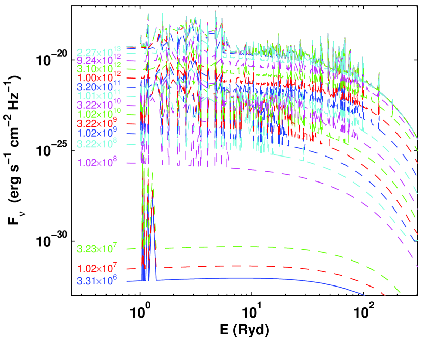
Figure 2.— Emitted flux by partial shocks with $T=5\times 10^{6}~{}K$, $Z=1$ solar in the strong$-B$ limit. Different shock ages ($n_{0}t$) are shown by different curves. For ages lower than $2\times 10^{13}$ cm^-3 s the age is indicated next to the appropriate curve. The curves showing the emitted radiation for older shocks closely overlaps.

In Figure 3, I show the ionization parameter that the shock self-radiation produces in the radiative precursor as a function of shock age. Initially, the ionization parameter is very low, but it increases with shock age, until finally stabilizing at a value appropriate for the complete shock. Figure 4 shows the corresponding neutral fraction in the material entering the shock. Initially ($n_{0}t\lesssim 10^{8}$ cm^-3 s), the precursor gas is almost entirely neutral. The lack of free electrons leads to the initial inefficient radiation demonstrated in Figure 2. At later times, the neutral fraction begins to decrease. First, both free electrons and neutral hydrogen coexist in the precursor gas, making initial cooling and emissivity in the post shock layers very efficient. As the depth of the radiating layers increases, hydrogen becomes mostly ionized, and the cooling efficiency of the post-shock layers drops again. It always remains higher that the CIE cooling efficiency due to underionized metal species that are penetrating from the radiative precursor.

The initial post-shock cooling rates as a function of age are displayed in Figure 5. This figure confirms that initially the lack of free electrons suppresses the cooling rate. The cooling rises as the electron fraction grows, until a maximal value is obtained when both neutral hydrogen atoms and free electrons are abundant in the gas entering the shock. At later times, as the gas become highly ionized, the abundance of efficient coolant decreases and the cooling rate declines again.

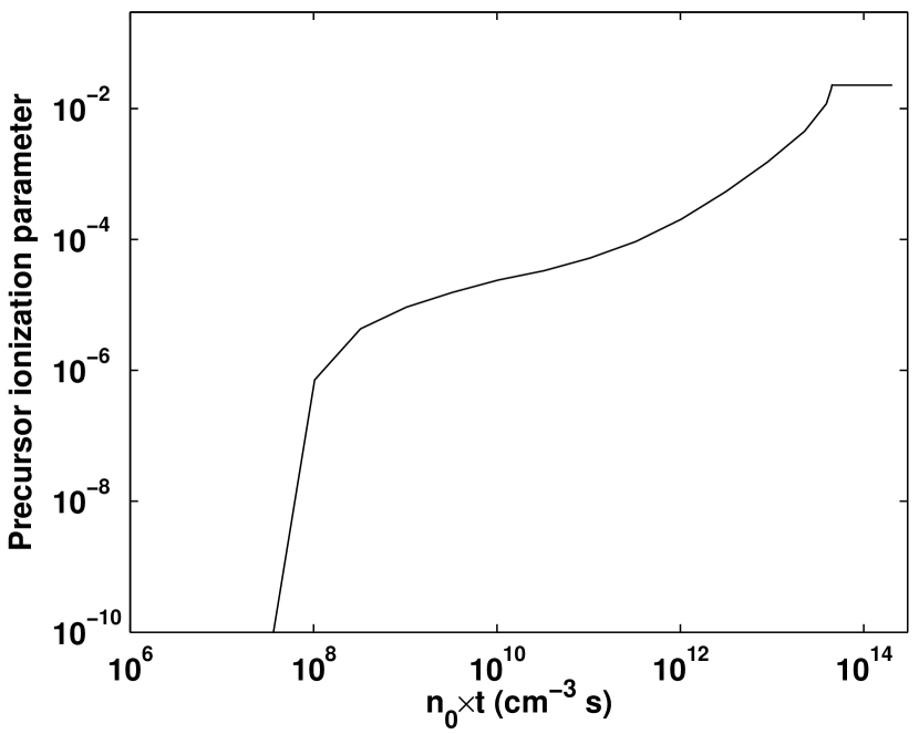
Figure 3.— Ionization parameter in the radiative precursor as a function of shock age for partial shocks with $T=5\times 10^{6}~{}K$, $Z=1$ solar in the strong$-B$ limit.

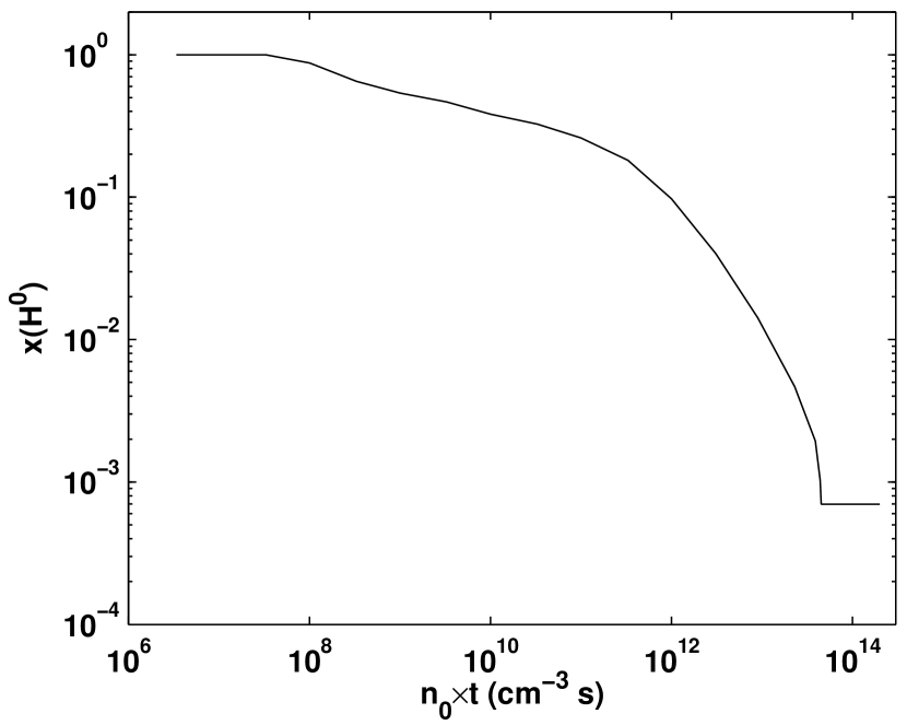
Figure 4.— Neutral fraction in gas entering shock, as a function of shock age for partial shocks with $T=5\times 10^{6}~{}K$, $Z=1$ solar in the strong$-B$ limit.

Figure 5.— The initial cooling rate (erg s^-1 cm^-3) as a function of shock age, for partial shocks with $T=5\times 10^{6}~{}K$, $Z=1$ solar in the strong$-B$ limit.

Figure 6.— Temperature as a function of time for partial shocks with various ages for $T=5\times 10^{6}~{}K$, $Z=1$ solar in the strong$-B$ limit. (a) Initial evolution. Following the shock formation, the incoming electron electron fraction is small, and electron impact excitations are inefficient. Cooling becomes more rapid as the shock evolves and the incoming neutral fraction grows. (b) “Young” shocks. In these shocks both neutral hydrogen and electrons are abundant at the shock front. Younger shocks cool more efficiently due to hydrogen Ly$\alpha$ cooling. Older shocks contain a smaller neutral fraction. (c) “Old” shocks. The incoming gas is ionized. These shocks follow a part of the trajectory of the complete shock.

The impact that this has on the shock structure is demonstrated in Figure 6. The upper panel shows the initial shock structure following the shock formation. As mentioned above, initially the free electron fraction is negligible, and cooling is inefficient. With time, the electron fraction grows, and cooling becomes more efficient. For example, panel (a) shows that the initial cooling at an age of $n_{0}t=3.23\times 10^{7}$ cm^-3 s is more rapid than the cooling at $n_{0}t=1.02\times 10^{7}$ cm^-3 s.

For these early ages, the gas remains neutral in the post-shock cooling layers, as the ionization time is longer than the shock age. This is demonstrated in Figure 7, in which I show the final neutral hydrogen fraction, obtained at the maximum distance downstream from the shock front, as a function of the shock age. The figure shows that for ages $\lesssim 10^{8}$, the gas remains partially neutral for the duration of the shock age. At later times, two effects act to increase the final ionization. First, the shock age becomes longer than the ionization time-scale, and second the initial precursor neutral fraction declines. It is important to note that while the gas is being ionized, the self-radiation propagating upstream in the post-shock layers, which is not included in this computation, may affect the shock structure and ionization states. This only affects very young shocks (panel (a) in Figure 6), and therefore has little impact of the results presented in this paper.

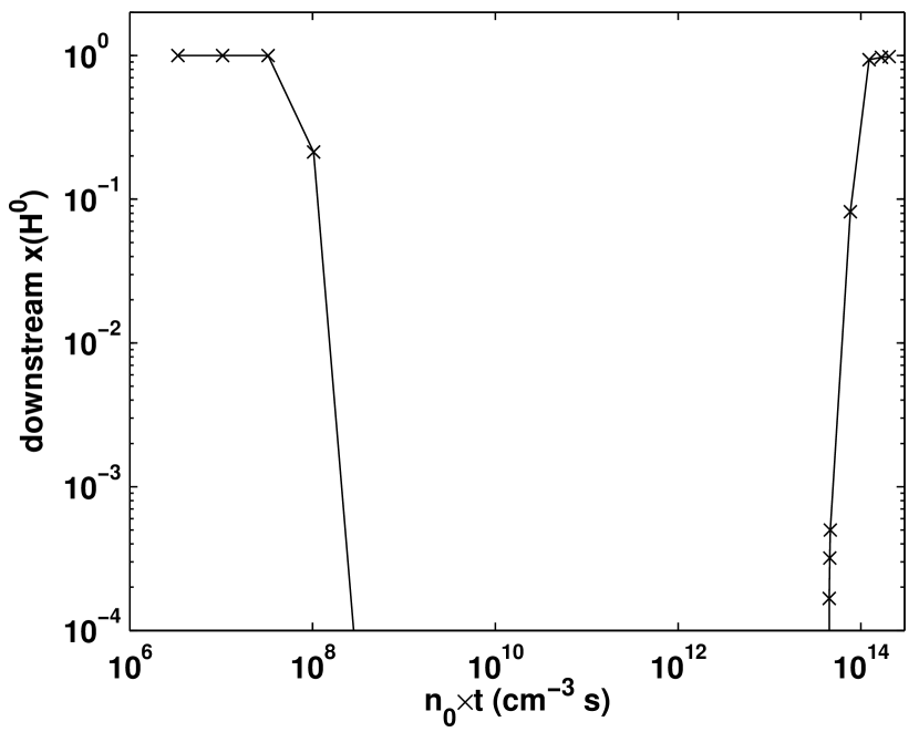
Figure 7.— The downstream neutral fraction as function of shock age, for partial shocks with $T=5\times 10^{6}~{}K$, $Z=1$ solar in the strong$-B$ limit.

Returning now to Figure 6. Once a significant electron fraction is established, the cooling depends on the availability of coolants in the precursor gas. This phase is shown by the middle panel. For a shock age of $10^{8}$ cm^-3 s, neutral hydrogen is abundant, and the initial cooling is very efficient, both due to collisional ionization and line cooling. This shock cools to a temperature of $\sim 3\times 10^{6}$ K within its life time. At later times, the shock self-radiation increases the ionization of the radiative precursor, and the initial post-shock cooling efficiency diminishes. The shortcomings of the quasi-static approximation are demonstrated in this panel. With the assumption that the age dependent structure may be approximated by a series of “self-contained” steady-states models, younger shocks cool to lower final temperatures than their older counterparts. For example, at an age of $9.2\times 10^{12}$  cm^-3 s, the shock only cools down to $\sim 4\times 10^{6}$ K. This inaccuracy in the temperature profile computations diminishes for older shocks, where the self-radiation and associated precursor ionization stabilize and are no longer a strong function of shock age. Because the self-radiation depends more on the total age of the shock and on the metal abundance (rather than on the details of the temperature profile), the computed self-radiation is not significantly affected by the quasi-static approximation. As I discuss below, the predicted column densities and resulting absorption line signatures are also independent of the quasi-static approximation.

After $\sim 10^{13}$ cm^-3 s, the shock self-radiation approaches its maximal intensity, and at later times any additional contribution to the shock self-radiation is negligible. The initial ionization states of the gas in the radiative precursor then depend only weakly on the shock age, and no longer affect the dynamical evolution of the shock. This is shown in the bottom panel. The temperature profiles of all the shocks with ages larger than $9.24\times 10^{12}$  cm^-3 s overlap at early time. The arrows mark the ending points of partial shocks of various ages, and some labels are indicated near the arrows for guidance.

3.2. Gas Metallicity

The gas metallicity affects the shock structure in two major ways (GS09). First, the metal content affects the cooling efficiency. For high-metallicity shocks, cooling is dominated by metal-line emission. For $10^{4}\lesssim T\lesssim 10^{6}$ K and $Z\gtrsim 0.1$, permitted transitions dominate the gas emission, and the cooling is roughly proportional to $Z$. At lower gas metallicities, cooling is dominated by hydrogen and helium. Below $10^{4}$ K, cooling is dominated by metal fine-structure transitions even at low metallicities. The cooling times are then always roughly proportional to $Z$. Higher metallicity shocks therefore evolve more rapidly. The different cooling times also set the degree of non-equilibrium ionization in the cooling zone. Departures from equilibrium ionization are therefore larger at higher metallicities.

Second, while the total energy emitted by the complete shock is independent of gas metallicity ($F\propto n_{0}v_{s}^{3}$) and is set by the input energy flux into the flow, the spectral energy distribution of the shock self-radiation is a strong function of gas metallicity. For low-$Z$, the radiation is dominated by thermal bremsstrahlung emission. The resulting spectrum is therefore a smooth bremsstrahlung continuum, with very little features. At higher metallicities, the contribution of metal line emission increases. This has a major effect on the shape of the emitted spectrum. For example, Figure 2 demonstrates that the emission of a $T_{s}=5\times 10^{6}$ K, solar metallicity shock is dominated by numerous metal emission lines. This affects both the downstream ion fractions (for “old” enough shock) and the ionization states in the radiative precursor.

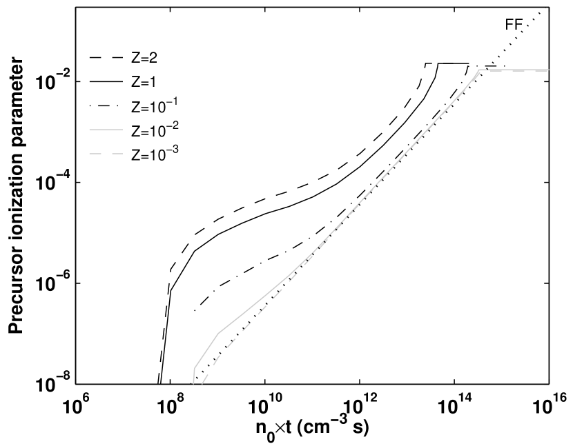
Figure 8.— Ionization parameter in the radiative precursor as a function of shock age for different gas metallicities, between $Z=2$ and $Z=10^{-3}$ times solar. The dotted curve shows the ionization parameter due to thermal bremsstrahlung emission at the shock temperature, $T_{s}=5\times 10^{6}$ K. The low metallicity results ($Z=10^{-3}$) overlap with the Bremsstrahlung predictions, but higher metallicity shocks produce larger ionization parameters due to line-emission.

Figure 8 shows how the changing spectral energy distribution affects the ionization parameter in the precursor gas. The different curves in Figure 8 show the precursor ionization parameter for different gas metallicities, as indicated by the labels, as a function of shock age. At low metallicities (grey curves) the ionization parameter is a simple power law in the shock age. This can be simply understood in terms of ionization by a thermal bremsstrahlung continuum. The thermal bremsstrahlung emissivity at the shock temperature (erg s^-1 cm^-3) is given by,

$$\varepsilon_{\rm FF}(\nu)=6.8\times 10^{-38}T_{s}^{-0.5}e^{h\nu/k_{\rm B}T_{s}}\;.$$ (1)

Assuming that a layer with depth $v_{\rm ps}\times t$ radiates with the above emissivity, the ionization parameter can be approximated by,

$$U_{\rm FF}=\int{\frac{\varepsilon_{\rm FF}(\nu)v_{\rm ps}}{h\nu}}\;\frac{1}{c}\;t\;d\nu\;,$$ (2)

where $v_{\rm ps}$ is the initial post-shock velocity. This simple approximation is shown by the dotted line is Figure 8 (denoted “FF”).

The results for $Z=10^{-3}$ overlap with the predicted bremsstrahlung ionization parameter. However, higher metallicity shocks produce larger ionization parameters, as a large fraction of their initial energy flux is emitted via line emission at ionizing energies, and a smaller fraction is emitted as high-energy free-free photons. For example, the solar metallicity curve (solid) is higher by $0.5$ to $2$ dex compared with the bremsstrahlung predictions. This implies that the radiative precursor is more highly ionized at any age for higher metallicity shocks. The ionized faction, and implied initial cooling rates vary accordingly.

3.3. Shock temperature

To study the impact of the shock temperature on the shock structure and evolution, I compare the results presented in section 3.1 for $T_{s}=5\times 10^{6}$ K with a model of a $5\times 10^{7}$ K shock. The overall characteristics of the hotter shock are similar to those discussed above. However, the shock temperature, and associated velocity, affect the initial energy content of the shock. Hotter shocks therefore have longer overall cooling times. For example, in the $5\times 10^{7}$ K shock the initial temperature is $10$ times higher, and the velocity is $10^{1/2}$ times higher than in the $5\times 10^{6}$ K shock. The total energy flux input is therefore $\sim 30$ times larger. This affects the total cooling time of the shock.

The emitted radiation field is also a strong function of the shock temperature. It is affected by the increased initial temperature. Above $\sim 2\times 10^{7}$ K, bremsstrahlung is the dominant emission process in CIE even at high metallicities. In complete shocks, the thermal energy distribution is therefore dominated by a hard free-free continuum. This continuum extends to higher energies than for $5\times 10^{6}$ K, because the exponential cut-off occurs at higher temperatures. The spectrum is also considerably smoother, because a large fraction of the initial energy flux is emitted as bremsstrahlung continuum, and the intense line emission that occurs at lower temperatures as the gas cools only provides a small contribution.

For partial shocks, however, line emission may play a dominant role even at $T_{s}=5\times 10^{7}$ K shocks. Figure 9 shows the emitted radiation as a function of shock age for a $5\times 10^{7}$ K, solar metallicity shock in the strong-$B$ limit. After the gas becomes partially ionized ($n_{0}\times t\geq 3.3\times 10^{9}$ cm^-3 s) the increased availability of metal lines coolants produces a significant emission-line UV-bump in the resulting spectrum. This is possible due to the highly underionized precursor that obtains at early times, before the full intensity of the shock self-radiation has accumulated. At later times, as the shock self-radiation efficiently ionizes the precursor gas, the fractional contribution of metal lines decrease, and a smoother spectrum is produced. For $3.2\times 10^{12}<n_{0}\times t<5.2\times 10^{14}$ cm^-3 s, the precursor gas is ionized, but the shocked-gas temperature is everywhere high enough to impede significant contribution of lines. At later times, at the gas cools in the post-shock flow, metal lines again contribute significantly to the emitted spectrum. The resulting spectrum has a lower line-to-continuum contrast, and extend to higher energies than the $5\times 10^{6}$ K shock (c.f. Figure 2).

Figure 9.— Emitted radiation for a $T_{s}=5\times 10^{7}$ K, $Z=1$ shock in the strong-B limit. At early times, the precursor gas is significantly underionized, leading to efficient line emission following the shock. However, as the gas ionization level increases, the post-shock radiation at $5\times 10^{7}$ K becomes dominated by thermal bremsstrahlung.

In Figure 10, I show how these spectral variations affect the ionization parameter in the radiative precursor. The different curves in Figure 10 show the precursor ionization parameter as a function of shock age for gas metallicities between $10^{-3}$ and $2$ times solar. As before, I compare these numerically computed ionization parameters with the expectation from a pure bremsstrahlung continuum at the shock temperature (see equations 1-2) shown by the dotted line. The low metallicity results are again consistent with the predictions of the free-free continuum. However, as opposed to the results presented in Section 3.1 for the $5\times 10^{6}$ K shock, Figure 10 shows that for $T_{s}=5\times 10^{7}$ K, the late time (age $\gtrsim 10^{12}$ cm^-3 s) results for high-$Z$ are also nicely consistent with the bremsstrahlung expectations. As discussed above, this is because at high temperatures, a large faction of the initial energy is radiated as free-free emission, and the total contribution of metal emission lines is smaller. At early times, when underionized gas rich with low-ionization species enters the shock front, the line contribution to the spectral energy distribution for high metallicity shocks remains significant.

For comparison, the thick gray curve shows the results for a $5\times 10^{6}$ K shock. The final ionization parameter produced by the hotter shock is considerably larger, as the higher energy content of the faster shock is radiated away.

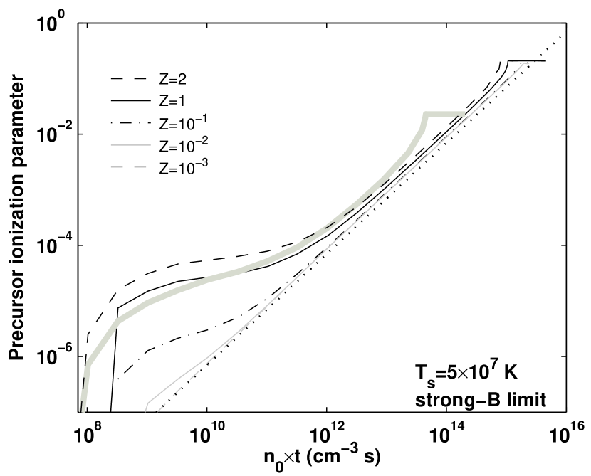
Figure 10.— The precursor ionization parameter in a $T_{s}=5\times 10^{7}$ K shock in the strong-B limit. The different curves show the ionization parameter for different gas metallicities as a function of shock age. The dotted curve shows the ionization parameter due to thermal bremsstrahlung emission at the shock temperature, $T_{s}=5\times 10^{7}$ K. The low metallicity results ($Z=10^{-3}$) overlap with the Bremsstrahlung predictions. However, at late times even the high-$Z$ cases agree with the bremsstrahlung predictions. For comparison, the thick gray curve shows the ionization parameter for $T_{s}=5\times 10^{6}$ K.

3.4. Magnetic field

The results presented so far have demonstrated the characteristics of shocks in the strong-$B$ (isochoric) limit. Shock for which $B=0$ evolve differently at late times. The most important difference is that when $B=0$, the pressure remains nearly constant, and the density increases as the gas cools. Since the cooling time is inversely proportional to the gas density, this implies rapidly decreasing cooling times (fast cooling) within the flow. The overall cooling times are much shorter, and in particular, the evolution below $10^{4}$ K is compressed into a very short time interval.

The final evolution of $B=0$ shocks is affected not only by the shorter cooling times, but also by the difference in downstream ionization parameter, $\propto F/n$. For strong-$B$ shock, the density in the flow is constant and the ionization parameters is $\propto v_{s}^{3}$. For $B=0$, the density increases as the gas cools, and the ionization parameter is therefore $\propto v_{s}^{3}n_{0}/n$, a factor $n_{0}/n$ smaller. Photoionization in the downstream layers is much less important when $B=0$. For the nearly isobaric evolution that obtains when $B=0$, $n_{0}/n\propto T/T_{0}$. The ionization parameter and resulting ion fractions are therefore significantly affected in the downstream gas after significant cooling has occurred. However, the differences in the post-shock ionization structure at early ages, before much cooling took place, remain small.

A second effect is related to the $PdV$ work that appears in $B=0$ shocks. The work done on the cooling gas implies that the overall emitted radiation is $5/3$ times larger for $B=0$ shocks than for isochoric shocks. Other than this $5/3$ scaling in the intensity of the integrated emission, however, the radiation emitted by $B=0$ shocks is similar to that produced by shocks in the strong-$B$ limit. The ionization in the radiative precursor is thus nearly independent of magnetic field.

Figure 11 demonstrated both points. It compares the precursor ionization parameter for $B=0$ (gray dashed curve) and for the strong-$B$ limit (solid curve). Despite the differences in the dynamical evolution, the two curves overlap at early times. It is only at late times that differences between the two cases arise. The final ionization parameter for $B=0$ is $5/3$ times larger than in the strong-$B$ limit, due to contribution of the $PdV$ work.

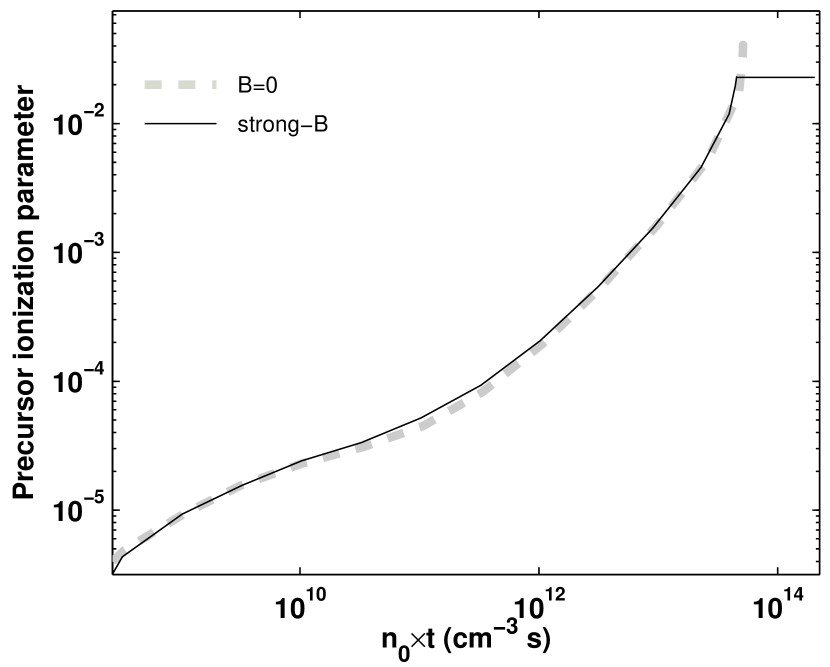
Figure 11.— A comparison of the precursor ionization parameter for $B=0$ (gray dashed line) and in the strong-B limit, for shocks with $T_{s}=5\times 10^{6}$ K and solar metallicity. The two curves nearly overlap at early times. The final ionization parameter of the complete shock is $5/3$ times higher when $B=0$, due to $PdV$ work.

4. The Ionization States and Metal Columns in a Strong-B, $5\times 10^{6}$ K, Solar Metallicity Shock

In this section I present computation of the integrated post-shock metal-ion columns produced in a strong-$B$ shock with $T_{s}=5\times 10^{5}$ K and solar metallicity. As an example, I discuss the formation of C III and C IV behind the shock front. Figure 12a shows the C III and C IV column densities created in the post-shock cooling layers as a function of shock age. For ages shorter than $\sim 10^{8}$ cm^-3 s, C III and C IV are not created behind the shock. At this age, there is a rapid increase in the column, which later stabilizes at a level of $\sim 10^{12}$ cm^-2. The columns then remain nearly constant for $\sim 10^{13}$ cm^-3 s. After that, the C III and C IV columns decrease, before rising again to achieve the levels observed in the complete shock.

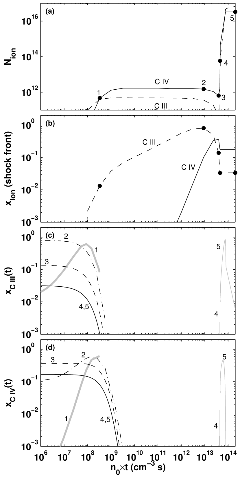
Figure 12.— (a) Column densities versus shock age for a $T=5\times 10^{6}~{}K$, $Z=1$ solar metallicity shock in the strong$-B$ limit. The dashed curve is for C III and the solid curve for C IV. (b) Ion fraction at the shock front as a function of shock age. (c) C III ion fraction as a function of time in five shock models. The final ages of the shocks shown here are indicated by the filled symbols in the top panel, and marked “1”-“5”. The thick gray curve is for a shock age of $3\times 10^{9}$ cm^-3 s (“1”); The dash-dotted curve is for $\sim 10^{12}$ cm^-3 s (“2”); the dashed curve is for $3.9\times 10^{13}$ cm^-3 s (“3”); the dark solid curve is for $4.5\times 10^{13}$ cm^-3 s (“4”); and the thin gray curve is for the complete shock (“5”). The curves for the last two cases overlap at early times. (d) Same as (c) but for C IV.

To explain this behavior, the evolution of the carbon ion fractions in the post-shock cooling layers must be understood. I focus on five representative ages, marked by the filled symbols in panel (a). These representative ages are $3\times 10^{9}$ cm^-3 s (“1”); $\sim 10^{12}$ cm^-3 s (“2”); $3.9\times 10^{13}$ cm^-3 s (“3”); $4.5\times 10^{13}$ cm^-3 s (“4”); and the complete shock (“5”).

Panel (b) shows the corresponding initial precursor C III and C IV ion fractions as a function of shock age. C III is efficiently produced in the radiative precursor at times later than $\sim 10^{8}$ cm^-3 s. Before that, the ionization parameter is smaller, and lower ionization states of carbon dominate its ion distribution. C III reaches the peak of its precursor abundance at a shock age of $\sim 10^{13}$ cm^-3 s, after which it is replaced by C IV. At $\sim 4\times 10^{13}$ cm^-3 s C IV is replaced by even higher stages of ionization. The five representative times are shown on the C III abundance curve for comparison.

In the post shock cooling layers, the gas adjusts to CIE at the shock temperature. At $5\times 10^{6}$ K, the most abundant carbon ion in CIE is fully stripped carbon (C⁶⁺). Given sufficient time, the shocked gas will approach the CIE ionization state. At very early times ($<10^{8}$ cm^-3 s) when the radiative precursor is effectively neutral and the free electron fraction is negligible (see Section 3), the shocked gas cannot efficiently cool or become ionized. Therefore, despite the initially neutral carbon ionization, no C III and C IV are produces in the cooling layers during the shock’s short lifetime. After this time, the post-shock gas does contain a significant fraction of free electrons, and the ionization and cooling processes become more rapid. At this stage, the gas can rapidly adjust to CIE near the shock temperature. The initial carbon ion distribution, which is dominated by low and intermediate-ions, is rapidly replaces by high-carbon-ions, until the carbon ion fractions finally establish the appropriate CIE distribution. Some amounts of C III and C IV are produced in this rapid initial ionization stage during which the gas adjust to CIE at the shock temperature. This is the column density seen in points “1” and “2” in panel (a). Because these initial columns are produced over an ionization time scale which is significantly shorter than the shock age, they are insensitive to the exact temperature profile of the post-shock gas, and are not significantly affected by the quasi-static approximation.

The specific ion distributions are shown in panels (c) (for C III) and (d) (for C IV); These panels follow the ion fractions as a function of time (not age) for the different shock ages shown in panels (a) and (b). For example, curve “1” corresponds to a shock age of $3\times 10^{9}$ cm^-3 s. Panel (b) shows that at this age, the initial C III ion fraction is $\sim 10^{-2}$, and the initial C IV ion fraction is negligible. The precursor carbon ion distribution is dominated by lower ionization states. Panel (c) shows that the C III abundance initially grows as the gas get more highly ionized, until it decreases again to be replace by C IV (panel (d)). The resulting column densities are shown in panel (a).

Point “2” shows a later age, for which the precursor C III ion fraction is at its peak, and the C IV abundance is also significant (panel b). Panel (c) the shows that C III, which starts at its peak abundance, is rapidly replaced by C IV (panel (d)), which in turn is later replaced by higher ionization states. Point “3”, at an age of $3.9\times 10^{13}$ cm^-3 s, is right at the minimum of the C III and C IV column densities. Panel (b) shows that at this age the radiative precursor is ionized enough that C IV is the dominant ion, whereas the abundance of C III is already reduced. Panel (c) shows that after starting at an abundance of $\sim 0.1$, C III is rapidly replaced by the initially dominant C IV. The ion fraction of C III is everywhere lower than that which existed at the age shown by point “2”, thus explaining the reduction in the column density associate with this initial post-shock ionization stage.

Finally, in ages “4” and “5”, the shock exists for long enough to allow for the production of C III and C IV in the downstream recombination layers of the shock. Even though the contribution of the initial ionization stage to the total column is lower than it was at earlier times, the contribution from late-time production of these ions, which spans a considerably larger path length, causes the rapid and substantial increase in the columns seen in panel (a). Finally (point 5) the total columns approach the values obtained in the complete shock.

Figure 13 shows examples for the column densities produced in partial shocks with $T_{s}=5\times 10^{6}$ K, $Z=1$, in the strong-$B$ limit. The dark curves show the columns densities produced in the post-shock cooling layers as a function of shock age. The dotted curves corresponds to C IV (and shows the same curve displayed in Figure 12). The other curves are for N V, O VI, and Ne VIII. Figure 13 also displays the column densities produced in the radiative precursor due to the shock self-radiation as a function of shock age. These are shown by the gray curves. It is clear from Figure 13 that significant amounts of intermediate/high ions are produced in the radiative precursor before similar columns are produced in the post-shock cooling layers. For example, at an age of $2\times 10^{12}$ cm^-3 s, the precursor C IV column density is $\sim 10^{14}$ cm^-2, whereas the post-shock column at this age is only $\sim 10^{12}$ cm^-2.

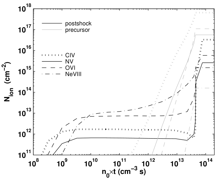
Figure 13.— Post-shock and precursor column densities (cm^-2) as a function of shock age ($n_{0}\times t$) for C IV, N V, O VI, and Ne VIII. in a $T=5\times 10^{6}~{}K$, $Z=1$ shock in the strong$-B$ limit.

5. Metal Columns in the Post-Shock Cooling Layers

In this section I present computations of the integrated metal column densities produced in the post-shock cooling layers. In computing the columns, I integrate from the shock front to the distance reached by the gas at the shock age. Older shocks extend over larger path-lengths and therefore yield larger total columns. The complete shocks are integrated to a distance where the gas has cooled down to the termination temperature, $T_{\rm low}=1000$ K.

The integrated metal ion column densities, $N_{i}$, through the post-shock cooling layers are given by

$$N_{i}=\int_{0}^{\rm age}n_{\rm H}ZA_{\rm el}x_{i}vdt\;,$$ (3)

where $n_{\rm H}$ is the hydrogen density, $A_{\rm el}$ is the abundance of the element relative to hydrogen in solar metallicity gas, $X_{i}$ is the ion fraction, and $v$ is the gas velocity. The integration is over time, where

$$dt\propto\frac{dT}{n\Lambda(x_{i},T,Z)}\;.$$ (4)

The mass-continuity equation implies that $n_{\rm H}v$ is constant throughout the flow, and the columns may therefore be expressed as

$$n_{i}\propto Z\int_{T_{\rm age}}^{T_{s}}x_{i}\frac{dT}{n\Lambda}\;.$$ (5)

As discussed in GS09, when $B=0$ the cooling times are shortened as the gas is compressed during cooling, and the column densities of ions produced at low temperatures are significantly suppressed compared with strong-$B$ shocks.

I list the full set of post-shock column densities as a function of shock temperature, metallicity, magnetic field and age in Tables 2, as outlined by Table 3. As examples, in Figures 14-18, I show the C²⁺, C³⁺, N⁴⁺, O⁵⁺, and Ne⁷⁺ post-shock column densities as a function of shock age, for the various shock models considered here.

Table 2Post-Shock Columns vs. Age

Age	$N($H${}^{0})$	$N($H${}^{+})$	$N($He${}^{0})$	…
(cm-3 s)	(cm-2)	(cm-2)	(cm-2)	(cm-2)
$1.000\times 10^{8}$	$9.0\times 10^{14}$	$6.7\times 10^{14}$	$7.9\times 10^{13}$	…
$3.300\times 10^{8}$	$5.4\times 10^{14}$	$4.4\times 10^{15}$	$5.3\times 10^{13}$	…
$1.000\times 10^{9}$	$4.1\times 10^{14}$	$1.5\times 10^{16}$	$3.3\times 10^{13}$	…

Note. — The complete version of this table is in the electronic edition of the Journal. The printed edition contains only a sample. The full table lists post-shock columns as functions of shock age for the $B=0$ and strong-B limits, for shock temperatures of $5\times 10^{6}$ K and $5\times 10^{7}$ K, and for $Z=10^{-3}$, $10^{-2}$, $10^{-1}$, $1$, and $2$ times solar metallicity gas (for a guide, see Table 3).

Table 3Post-Shock and Precursor Columns Tables

			Post-Shock	Precursor
Data			Columns	Columns
$5\times 10^{6}$ K	strong-$B$	$Z=2$	2A	4A
		$Z=1$	2B	4B
		$Z=10^{-1}$	2C	4C
		$Z=10^{-2}$	2D	4D
		$Z=10^{-3}$	2E	4E
	$B=0$	$Z=2$	2F	4F
		$Z=1$	2G	4G
		$Z=10^{-1}$	2H	4H
		$Z=10^{-2}$	2I	4I
		$Z=10^{-3}$	2J	4J
$5\times 10^{7}$ K	strong-$B$	$Z=2$	2K	4K
		$Z=1$	2L	4L
		$Z=10^{-1}$	2M	4M
		$Z=10^{-2}$	2N	4N
		$Z=10^{-3}$	2O	4O
	$B=0$	$Z=2$	2P	4P
		$Z=1$	2Q	4Q
		$Z=10^{-1}$	2R	4R
		$Z=10^{-2}$	2S	4S
		$Z=10^{-3}$	2T	4T

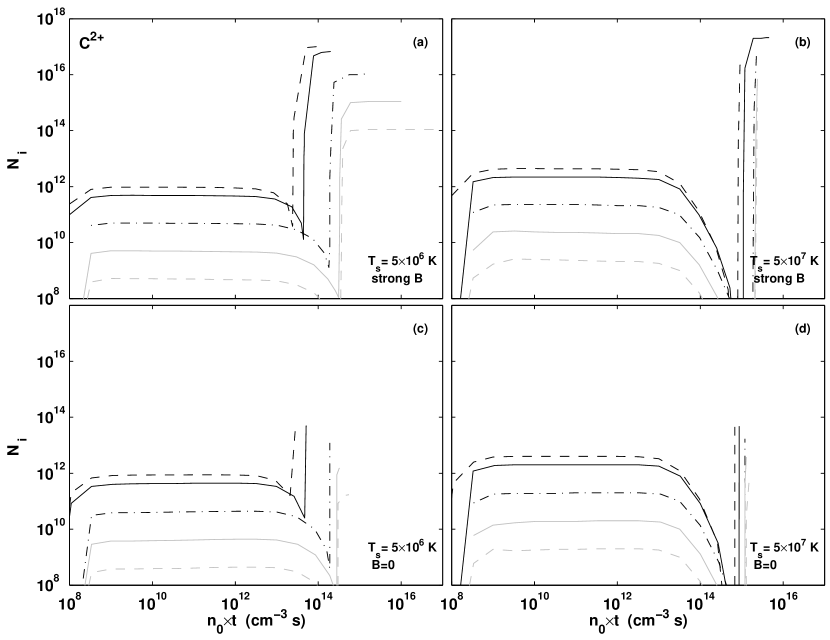
Figure 14.— Post-shock C²⁺ columns as a function of shock age for $Z$ from $10^{-3}$ to $2$ times solar. (a) $T_{s}=5\times 10^{6}~{}K$, strong-$B$. (b) $T_{s}=5\times 10^{7}~{}K$, strong-$B$. (c) $T_{s}=5\times 10^{6}~{}K$, $B=0$. (d) $T_{s}=5\times 10^{7}~{}K$, $B=0$.

Figure 15.— Same as Figure 14, but for C³⁺.

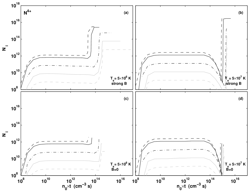
Figure 16.— Same as Figure 14, but for N⁴⁺.

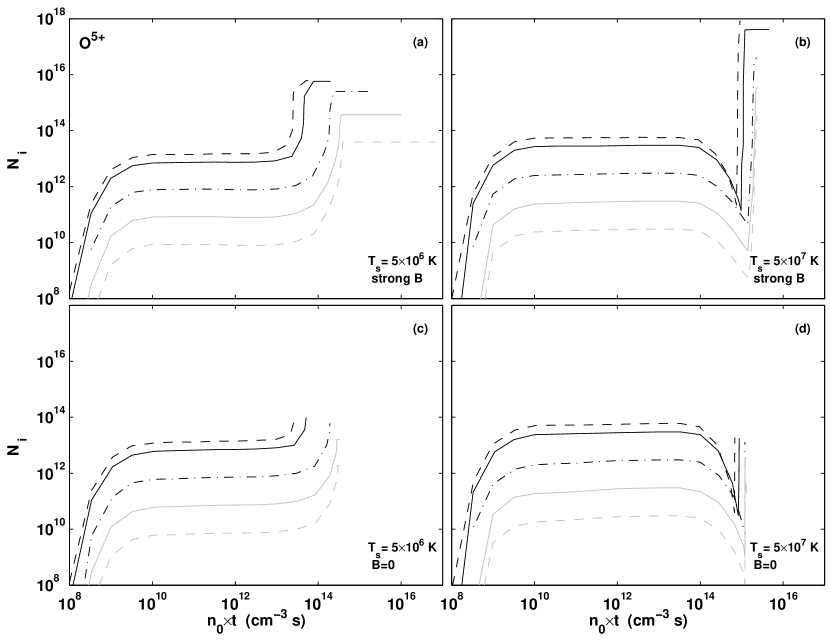
Figure 17.— Same as Figure 14, but for O⁵⁺.

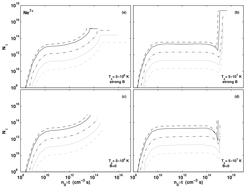
Figure 18.— Same as Figure 14, but for Ne⁷⁺.

Focus for example on Figure 15. This figure confirms that the C³⁺ column is gradually built out of two components (see discussion in Section 4). Initially, C³⁺ peaks as the gas is ionized after passing the shock front. This first abundance peak is short, and rapidly builds up a low column density, that then remains roughly constant with little additional contribution as the shock ages because higher stages of ionization dominate the ion abundance. Finally, when the shock age is large enough to allow the gas to cool behind the shock front, a second abundance peak is produced in the recombining layers. This second peak is much longer, and produces the significant column observed in the complete shocks (see Section 4 for details). For example, panel (a) shows that for $T_{s}=5\times 10^{6}$ K and $Z=2$, the C³⁺ column that is produced during the initial ionization stage is $\sim 10^{12}$ cm^-2. This column is built up over $<10^{9}$ cm^-3 s, and then remains constant as higher ionization states of carbon dominate in the hot radiative zone. Finally, when the shock age reaches $\sim 3\times 10^{13}$ cm^-3 s, a second C³⁺ is produced in the cooling layers. This second dominant peak accumulates to a column density of $\sim 5\times 10^{16}$ cm^-2 for the complete shock.

The post-shock column densities are unaffected by the quasi-static approximation, because the initial abundance peaks occur over a time scale shorter than the shock-age, and are therefore insensitive to the details of the temperature profile, whereas the second dominant abundance peaks are produces at late times within the nonequilibrium cooling zone and the photoabsorption plateau, when the quasi-static approximation robustly holds.

Higher ionization states, that exist at or near the shock temperature are accumulated more gradually over the shock age. For example, panel (a) of Figure 18 shows that in a $5\times 10^{6}$ K shock, the Ne⁷⁺ column density increases monotonically with time. This is because Ne⁷⁺ is abundant even within the hot radiative zone, and its column density therefore accumulates more gradually. The Ne⁷⁺ abundance peaks at a temperature of $6\times 10^{5}$ K, and indeed a rapid growth in its column can be seen at later times as the shocked gas cools through this temperature.

5.1. Gas Metallicity

As discussed above, the gas metallicity affects the ion fractions produced in the post-shock cooling layers in several ways. First, higher metallicity gas cools more efficiently. This results in shorter cooling times, and in increased recombination lags. Second, the spectral energy distribution of the shock self-radiation is dominated by line-produced UV-photons for high metallicity gas, and by a harder thermal bremsstrahlung spectrum for lower-Z cases. Photoionization is therefore more efficient in higher-metallicity shock, which produce larger ionization parameters (see also Figure 8).

For the column density distributions shown in Figures 14-18, a distinction must be made between the first and second abundance peaks discussed above. The first column peak is accumulated over an ionization time scale at the shock temperature. This ionization time-scale does not depend on the gas metallicity, and is barely affected by gas cooling, because little cooling occurs so rapidly. The integrated metal ion column densities are therefore simply proportional to the gas metallicity (see Equation 5). This can clearly be seen in Figures 14-18.

The second abundance peak occurs during the post shock cooling layers. The duration of this second peak is determined by the cooling time at the temperature where the ion is produced. Equations 5 shows that when the cooling function $\Lambda$ is proportional to $Z$ (when metals dominate the cooling) the columns are nearly independent of gas metallicity. This is because when $\Lambda\propto Z$, reduced elemental abundances are compensated by longer cooling times, and $Z$ cancels out in Equation 5. The actual behavior is more complicated than that, because the ion distributions themselves are functions of gas metallicity, due to departures from equilibrium ionization, and because of the different spectral energy distributions of the photoionizing self-radiation.

On the other hand, when the cooling efficiency is independent of $Z$ (because it is dominated by hydrogen/helium cooling or by thermal bremsstrahlung), Equation 5 indicates that the metal-ion columns should be proportional to $Z$.

Figures 14-18 confirm that for $B=0$ (when photoionization does not significantly affect the ion distributions, see below) the final column densities are only weakly dependent of metallicity when $Z\gtrsim 0.1$ (i.e. metal dominate the cooling and $\Lambda\propto Z$), and are roughly proportional to $Z$ for lower metallicities (when H/He dominate the cooling).

5.2. Shock temperature

The shock temperature has a strong impact on the ion fractions and resulting column densities produced in the post-shock cooling layers. First, faster shocks give rise to more highly ionized species that are produced at or near the shock temperature. Second, as discussed in Section 3, the energy flux radiated by the (complete) shock is proportional to $v_{s}^{3}$ ($\propto T_{s}^{1.5}$). In addition, the spectral distribution of the shock self-radiation is harder for faster shocks. Hotter shocks therefore produce an abundance of high energy photons, that can efficiently photoionize the gas in the cooling layers.

Equation 3 implies that for ions that are produced near $T_{s}$, the metal columns will be proportional to the shock velocity. This can be seen for the initial peaks shown in Figures 14-18. The column densities produced in the initial peaks of the $5\times 10^{7}$ K shocks are a factor of $\sim 3$ ($\sqrt{10}$) larger than those produced in the $5\times 10^{6}$ K shocks. The complete column densities accumulated along the total cooling time of the shock are affected by other factors, most importantly photoionization by the shock self-radiation. This affects the ion distributions $x_{i}$ in Equation 5.

5.3. Magnetic field

The strength of the magnetic field is one of the parameters that determines the significance of photoionization in the post-shock gas. In strong-$B$ shocks, the isochoric evolution ensures that the accumulated shock self-radiation propagates into constant density gas. However, when $B=0$ the gas is compressed as it cools, and the density in the photoabsorption plateau is significantly larger than $n_{0}$. The ionization parameter is accordingly lower, by a factor $T_{s}/T$. Photoionization is therefore very important in strong-$B$ shocks, but does not play a significant role when $B=0$. In addition, the extent of the photoabsorption plateau is considerably shorter when $B=0$, due to the faster cooling that takes place in the compressed gas.

As discussed above, Equation 3 implies that the column densities of intermediate and low ion are significantly suppressed when $B=0$ compared to isochoric strong-$B$ limit. This is confirmed by the final (complete shock) columns shown in Figures 14-18. For example, for a $5\times 10^{6}$ K shock in solar metallicity gas, a C IV column $>10^{16}$ cm^-2 is created in the strong-$B$ limit, but this column is only $\sim 10^{12}$ cm^-2 when $B=0$. However, as discussed above, the initial evolution of the post-shock ion fraction following the shock front is not expected to depend on the intensity of the magnetic field. Photoionization does not play an important role in the hot radiative zone, and no significant compression takes place when $T\sim T_{s}$. The initial columns are indeed very similar between the upper and lower panels of Figures 14-18.

6. Metal Columns in the Radiative Precursor

In this section I present the equilibrium photoionization column densities that are produced in the radiative precursors. The precursor gas is heated and photoionized by the shock self-radiation propagating upstream. This upstream radiation is gradually being absorbed by the precursor gas, producing a photoabsorption layer in which the heating and ionization rates gradually decline with increasing (upstream) distance from the shock front.

For optically thin shocks, I use the post-shock flux at the position associated with the shock age, $l_{\rm age}$, for the upstream radiation field. For older shocks that become thick to their self-radiation, I use the post-shock flux at the position where the gas first becomes thick at the Lyman limit, $l_{\rm thick}$. Downstream of $l_{\rm thick}$, the radiation field is attenuated by absorption in the post-shock photoabsorption plateau.

For each shock model, I construct an equilibrium photoionization model assuming that the appropriate flux enters a gas of uniform density $n_{0}/4$. The typical temperatures in the radiative precursor are in the range $10^{4}-10^{5}$ K, and I integrate from the shock front to a distance where absorption reduces the heating rate sufficiently for the gas to reach a temperature $T_{\rm low}=1000$ K.

To compute the photoionization ion fractions in the radiative precursors, I use the photoionization code Cloudy (ver. 07.02.00) to construct equilibrium models of the precursor absorbing layers. The ionization parameter in the radiative precursors are larger than in the corresponding downstream photoabsorption plateaus, because the gas density in the precursor is four times lower. Intermediate and low ions may therefore be produced more efficiently in the precursor compared to the post-shock cooling layers, and the precursor may dominate the total observed columns of such ions even for complete shocks (GS09). For partial shocks, the column density of intermediate ions in the radiative precursor builds up even before the post-shock gas cools to produce the photoabsorption plateus. In such cases, UV absorption line signatures may be produced by the radiative precursor while the shock gas is still too hot to be efficienctly observed.

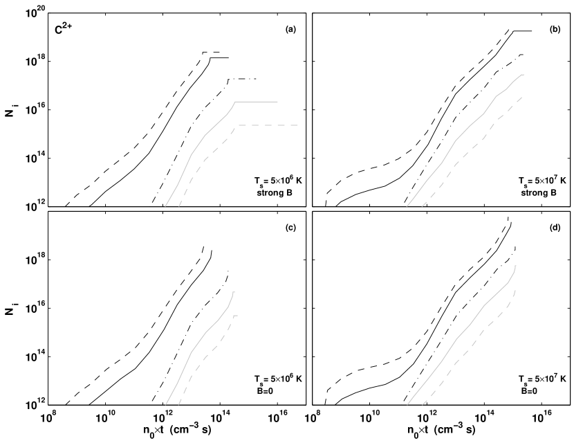
Figure 19.— Precursor C²⁺ columns as a function of shock age for $Z$ from $10^{-3}$ to $2$ times solar. (a) $T_{s}=5\times 10^{6}~{}K$, strong-$B$. (b) $T_{s}=5\times 10^{7}~{}K$, strong-$B$. (c) $T_{s}=5\times 10^{6}~{}K$, $B=0$. (d) $T_{s}=5\times 10^{7}~{}K$, $B=0$.

Figure 20.— Same as Figure 19, but for C³⁺.

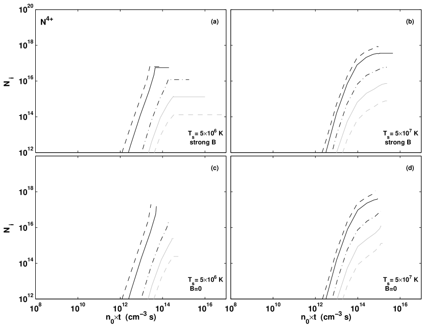
Figure 21.— Same as Figure 19, but for N⁴⁺.

Figure 22.— Same as Figure 19, but for O⁵⁺.

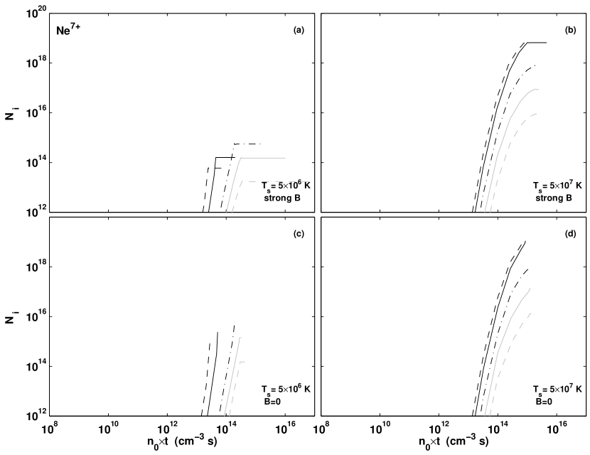
Figure 23.— Same as Figure 19, but for Ne⁷⁺.

Figures 19-23 display, as examples, the integrated precursor column densities of C²⁺, C³⁺, N⁴⁺, O⁵⁺, and Ne⁷⁺ as functions of the shock age (cm^-3 s), for $Z$ between $10^{-3}$ and $2$. The upper panels are for radiative precursors of strong-$B$ shocks, and the lower panels are for $B=0$. The left hand panels are for $T_{s}=5\times 10^{6}$ K, and the right hand panels for $T_{s}=5\times 10^{7}$ K. The full set of precursor column densities for all the metal ions that I consider are listed in Table 4 as outlined in Table 3.

Figures 19-23 confirm that as the flux entering the precursor accumulates with time, deeper precursors are produced. As expected, the precursor columns increase monotonically with shock age.

Table 4Precursor Columns vs. Age

Age	$N($H${}^{0})$	$N($H${}^{+})$	$N($He${}^{0})$	…
(cm-3 s)	(cm-2)	(cm-2)	(cm-2)	(cm-2)
$1.000\times 10^{8}$	$1.6\times 10^{17}$	$2.3\times 10^{16}$	$1.4\times 10^{16}$	…
$3.300\times 10^{8}$	$2.2\times 10^{19}$	$2.7\times 10^{18}$	$1.5\times 10^{18}$	…
$1.000\times 10^{9}$	$3.6\times 10^{19}$	$5.4\times 10^{18}$	$2.1\times 10^{18}$	…

Note. — The complete version of this table is in the electronic edition of the Journal. The printed edition contains only a sample. The full table lists precursor columns as functions of shock age for the $B=0$ and strong-B limits, for shock temperatures of $5\times 10^{6}$ K and $5\times 10^{7}$ K, and for $Z=10^{-3}$, $10^{-2}$, $10^{-1}$, $1$, and $2$ times solar metallicity gas (for a guide, see Table 3).

Figures 19-23 demonstrate that significant columns of low (e.g. C²⁺) and intermediate/high (e.g. C³⁺, N⁴⁺, O⁵⁺) ions are created in the radiative precursors. For example, a comparison of Figures 19 and 14 (note different scales) shows that the C²⁺ columns are dominated by the radiative precursors at all times. This is also the case for C³⁺ and N⁴⁺ for $n_{0}t\gtrsim 10^{12}$ cm^-3 s, and for O⁵⁺ at $n_{0}t\gtrsim 10^{13}$ cm^-3 s. However, for high-ions, which abundance peaks closer to $T_{s}$, the column densities are dominated by the post-shock cooling layers. For example, the Ne⁷⁺ CIE fractional abundance peaks at $\sim 6\times 10^{5}$ K, but it is abundant between $4\times 10^{5}$ and $4\times 10^{6}$ K (see Gnat & Sternberg 2007). Figures 23 and 18 confirm that for $T_{s}=5\times 10^{6}$ K, the Ne VIII column produced in the post-shock cooling layers dominates over the precursor column. This is because the equilibrium photoionization and heating rates in the precursor are too low to allow for the efficient production of Ne⁷⁺. However, for hotter $T_{s}=5\times 10^{7}$ K shocks (for which $T_{s}\gg T_{{\rm Ne}^{7+}}$), the Ne VIII column is again dominated by the radiative precursor, as the more intense and energetic radiation field produced by the hotter shocks efficiently ionize the precursor gas.

The column densities produced in the radiative precursors for strong-$B$ shocks are similar to those produced in $B=0$ precursors. The radiative fluxes in the two cases are similar, and differ only by a factor $5/3$ due to the $PdV$ work included in the $B=0$ shocks. A comparison of the upper and lower panels of Figures 19-23 indeed shows that the columns are similar for all ages.

The ratio between the precursor and post-shock columns is a strong function of shock age. Consider, for example, the C³⁺ columns shown in Figures 15 and 20. Figure 15a shows that readily detectable amounts of C IV ($\gtrsim 10^{13}$ cm^-2) are only produced in the post-shock cooling layers in the very final stages of the shock formation, as the shocked gas cools through the non-equilibrium cooling zone and photoabsorption plateau. For solar metallicity gas this occurs at $n_{0}t\sim 5\times 10^{13}$ cm^-3 s. However, in the radiative precursor detectable amounts of C IV are produced as early as $10^{12}$ cm^-3 s. This implies that there is a significant duration of time over which fast radiative shocks may be observed by means of their radiative precursor, even though the shocked gas itself was not able to cool, and therefore produces little observable signatures. A similar behavior is also observed for other gas metallicities, temperatures, and magnetic field properties.

I conclude that intermediate and high ions produced in the radiative precursors of fast shock waves may serve as means for identifying and detecting young shocks that have not yet existed over a cooling time, and for which the shocked gas remains hot and difficult to observe.

7. Diagnostics

Diagnostic diagrams for fast radiative shocks may be constructed using the computational data presented in Sections 5 and 6. In Figure 24 I show, as an example, “trajectories” for $N_{{\rm CIV}}/N_{{\rm OVI}}$ versus $N_{{\rm NV}}/N_{{\rm OVI}}$ for ages ranging from $\sim 3\times 10^{8}$ to $\sim 2\times 10^{14}$ cm^-3 s, assuming a $5\times 10^{6}$ K, $Z=1$, strong-$B$ shock. The shock age is represented by color along the curves from young (blue) to old (red). The trajectories are only shown at ages for which the absolute O VI column density is greater than $10^{11}$ cm^-2. The left panel is for the columns produced in the post-shock cooling layers, and the right panel is for the radiative precursor. Figure 24 shows that the ion ratios created in the radiative precursor may be very different from those which are produced in the post-shock gas. At early times ($n_{0}t\lesssim 5\times 10^{13}$ cm^-3 s), the column densities presented in Figure 24 are completely dominated by the precursor columns. At later times, the post-shock cooling layers also contribute to the observed columns.

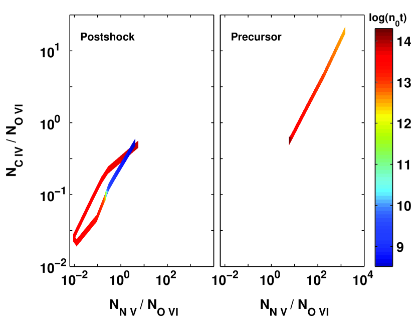
Figure 24.— Column density ratios $N_{{\rm CIV}}/N_{{\rm OVI}}$ vs. $N_{{\rm NV}}/N_{{\rm OVI}}$ is strong-$B$ shocks with $T=5\times 10^{6}$ and $Z=1$ solar. Shock age is indicated by color along the trajectories, from young (blue) to old (red). Age (cm^-3 s) vs. color legend is on the right. The left panel is for the shocked gas, and the right panel is for the radiative precursor. The trajectories are only shown at ages for which the O VI column is greater than $10^{11}$ cm^-2.

As demonstrated above, the UV-absorption line signatures are dominated by photoionized gas in the radiative precursor over a significant fraction of the shock lifetime. Ion-ratio diagrams, like the one shown in Figure 24, may serve as diagnostics for gas in the radiative precursors of incomplete, fast radiative shocks. The detection and identification of precursor gas may allow us to confirm the existence of hot, unobservable, shocked gas, and to infer the associated baryonic content.

8. Summary

In this paper, I present theoretical computations of the metal-ion column densities produced in the post-shock cooling layers, and in the radiative precursors of fast astrophysical shocks as a function of shock age. My shock models rely upon the code and methods presented in Gnat & Sternberg (2009; GS09), but relax the assumption of steady-state complete shocks. To attain steady-state, the shocks must exist over time-scales that are long compared with their cooling times. Otherwise the shock structure, emitted radiation and radiative precursors are a function of the shock age in the partially cooled shocks.

I approximate the evolution of the shock properties by assuming quasi-static evolution. For a given shock, as specified by the shock velocity, gas metallicity and magnetic field, I construct a series of models, each appropriate for a specific age, which are assumed to be independent of each other.

In these models, I use and extend the shock code developed in GS09. This code computes the time-dependent downstream ion fractions and cooling efficiencies, follows the radiative transfer of the shock self-radiation through the post-shock cooling layers, takes into account the resulting photoionization and heating rates, follows the one-dimensional dynamics of the flowing gas, and self-consistently computes the photoionization ion fractions in the radiative precursor. I follow the ion fractions of all ionization states of the elements H, He, C, N, O, Ne, Mg, Si, S, and Fe. I consider shock velocities of $600$ and $2000$ km s^-1, associated with shock temperatures of $5\times 10^{6}$ and $5\times 10^{7}$ K, and gas metallicities between $10^{-3}$ and $2$ times the heavy element abundance of the Sun.

For the dynamical evolution I consider shocks with no magnetic field ($B=0$), for which the gas evolves with nearly constant pressure, with $P_{\infty}=4/3\;P_{0}$, where $P_{0}$ is the post-shock pressure. I also consider shocks in which the magnetic field is dynamically dominant everywhere ($B/\sqrt{\rho}\gg v_{s}$) so that the pressure is dominated by the magnetic field, and the density remains constant in the flow. When $B=0$ the gas is compressed and decelerated as is cools. The increased density implies faster cooling, and the low-temperature evolution is significantly faster when $B=0$ compared with the strong-$B$ limit. In Section 2, I describe the equations that I solve, and the numerical method used to compute the shock properties.

In Section 3, I investigate the shock structure, and focus on how it depends on the shock age. Complete shocks are composed of several zones, through which the gas flows. The precursor gas enters the hot radiative zone, in which the gas is hot and cooling is inefficient. After a significant fraction of the shock input energy is radiated, the temperature finally declines, allowing the cooling rate to increase. The gas then goes through the nonequilibrium cooling zone, in which cooling is very efficient, and recombination lags may occur. Once the neutral fraction rises, photoabsorption becomes efficient, and the gas enters a photoabsorption plateau in which the temperature profile is shallower, until finally all self-radiation is absorbed and the gas cools completely. In partial, time-dependent shocks, this classical picture is modified due to the finite shock age. The shock structure, self-radiation and precursor ionization then depend on the shock age.

The shock self-radiation accumulates over time, as deeper downstream layers contribute to the emitted radiation. Initially, the self-radiation of young shocks is faint, leading to low ionization parameters and large neutral fractions in their radiative precursors. In this case, the post-shock free electron abundance is small, leading to inefficient excitation and ionization in the downstream gas. As the intensity of the self-radiation increases, the neutral fraction in the radiative precursor diminishes. At this stage, both free electrons and neutral hydrogen atoms are abundant in the gas entering the hot radiative zone. Cooling due to both collisional ionization and Ly$\alpha$ emission is highly efficient under these conditions. Finally, once the shock self-radiation is intense enough to fully ionize the precursor hydrogen gas, the initial cooling drops again due to the lack of efficient coolants. Even then, cooling remains large compared with CIE, due to the underionized metal species that exist in the radiative precursor.

As expected, the ionization parameter in the radiative precursor increases monotonically with shock age as the shock self-radiation builds up. After the shock exists for a cooling time, the intensity of this radiation stabilizes at a value appropriate for the complete shock. I find that the precursor ionization parameter is a strong function of gas metallicity. For low metallicities, the shock self-radiation is composed almost entirely of thermal bremsstrahlung emission. The precursor ionization parameter is then a simple power law in the shock age. However, for larger metallicities, a significant fractions of the shock self-radiation is emitted as metal-lines, creating a “UV-bump” in the spectral energy distribution. The contribution of the metal-line emission enhances the ionization parameter, which may be between $0.5$ and $2$ dex larger than the bremsstrahlung value. Hotter shocks emit a larger fraction of their input energy as thermal bremsstrahlung even at high metallicities, and their ionization parameters are closer to the free-free values.

In Sections 4-5, I present computations of the integrated metal-ion column densities in the post-shock cooling layers. I examine how the downstream column densities evolve with time. I list the complete set of post-shock column densities in Table 2, as outlined in Table 3. For UV-detectable ions (C IV, N V, O VI etc.), the column densities are composed of two distinct contributions. First, some column density is initially created over a very short time scale (an ionization time-scale), as the underionized gas in the precursor approaches CIE at the shock temperature. This column density builds over a time scale which is orders of magnitudes shorter than the cooling time, and later remains constant as the shock evolves. For example, for C IV the initial column density in a $5\times 10^{6}$ K, $Z=1$, strong-$B$ shock is $\sim 10^{12}$ cm^-2. It accumulates over a time scale of $\sim 10^{9}$ cm^-3 s, and later remains constant for a few $10^{13}$ cm^-3 s. A second, dominant peak is later created as the shocked gas cools and recombines through the nonequilibrium cooling zone and the photoabsorption plateau. In the example above, the second peak yields a C IV column density of $\sim 3\times 10^{16}$ cm^-2, which is the column observed in a complete shock.

The initial peaks produce very low column densities which are difficult to observe. The columns in these initial peaks are roughly proportional to gas metallicity. The second dominant peak depends on the gas metallicity in a more complicated manner, related to the dominant coolants at various temperatures. The initial peaks are also insensitive to the value of the magnetic field, as they are created on an ionization time-scale over which very little evolution in the thermal and dynamical properties of the gas takes place. However, the second dominant peaks are strongly affected by the magnetic field. When $B=0$, the compression and associated accelerated cooling lead to significant suppression of intermediate and low ions created at low temperatures compared with constant-density, strong-$B$ shocks. High-ions, which are created at or near the shock temperature, do not depend on the value of the magnetic field. UV observations of shocked gas, and in particular the ratio of high to intermediate ions, may be used to probe the intensity of interstellar and intergalactic magnetic fields in complete fast shocks.

In Section 6, I compute the precursor column densities for the various shock models as functions of shock age. As expected, the column densities of the intermediate and high ions are monotonically increasing functions of the shock age. They grow as the intensity of the shock self-radiation accumulates with time, leading to more highly-ionized, deeper upstream absorption layers. I list the full set of precursor column densities in Table 4, as outlined in Table 3. I find that the precursor column densities of intermediate and low ions dominate the observable signatures from fast shocks over a significant fraction of the shock cooling time.

As opposed to the column densities created in the downstream cooling layers, the precursor column densities are insensitive to the value of the magnetic field. Because the shock self-radiation is dominated by emission in the hot radiative zone, in which no significant cooling takes place, the ionization parameter and spectral energy distributions are similar for strong-$B$ shocks and for shock in which $B=0$.

The results presented here demonstrate that over extended periods of time, the precursor produces observable amounts of intermediate and high ions, such as C IV, N V, and O VI. These precursor UV signatures may be the only means to detect and identify the existence of young fast shocks. For example, in a $5\times 10^{6}$ K, solar metallicity shock in the strong-$B$ limit, readily detectable amounts of C IV ($\gtrsim 10^{13}$ cm^-2) are only produced in the post-shock cooling layers at very late times, at ages $\gtrsim 5\times 10^{13}$ cm^-3 s. However, in the radiative precursor similar amounts of C IV are produced as early as $10^{12}$ cm^-3 s.

Finally, in Section 7, I demonstrate how ion-ratio diagrams may serve as diagnostics for gas in the radiative precursors of partially-cooled fast astrophysical shocks. This provides a mean to observationally identify the precursors of young fast shocks. I suggest that the detection and identification of precursor gas, photoionized by the hard shock self-radiation, may allow us to confirm the existence of the hot, unobservable, shocked counterpart. Absolute calibration of the observed precursor column densities may then be used to infer the shocked-gas column, and estimate the ”missing” baryonic mass associated with the shocks.

9. Conclusions

Shock waves are a common phenomenon in astrophysics, and have a profound impact on the energetics and distribution of gas in the interstellar and intergalactic medium. In this paper, I present theoretical computations of the metal-ion column densities produced in the post-shock cooling layers, and in the radiative precursors of fast astrophysical shocks as a function of shock age.

This work is motivated by recent UV and X-ray observations of gas that may be a part of a $10^{5}-10^{7}$ K “warm/hot intergalactic medium” (e.g. Tripp et al. 2007; Savage et al. 2005; Buote et al. 2009; Narayanan et al. 2009; Fang et al. 2010; Danforth et al. 2010). However, the results presented here are also applicable to other astrophysical environments in which young shocks are expected to prevail, including supernovae remnants and active galactic nuclei. The WHIM application is particularly interesting, because the warm/hot intergalactic medium is expected to be a major reservoir of baryons (e.g. Cen & Ostriker 1999; Davé et al. 2001; Bertone et al. 2008), and in fact account for the so-called “missing baryons” in the low-redshift Universe.

In my numerical models, the time-evolution of the shock structure, self-radiation, and associated metal-ion column densities are computed by a series of quasi-static models, each appropriate for a different shock age. The results for the post-shock and precursor columns are presented in convenient online format in Tables 2 and 4. For the post-shock columns, I use a shock code that explicitly follows the nonequilibrium ionization states in the post-shock cooling layer, taking into account the impact of the shock self-radiation, cooling, and gas dynamics. The precursor columns are set by photoionization equilibrium with the shock self-radiation, which depends on the shock parameters and age.

The shock models presented here are applicable to the shock-heated warm/hot intergalactic medium, and may provide a way to identify and measure some of the missing baryonic mass. My computations indicate that readily observable amounts of intermediate and high ions, such as C IV, N V, and O VI are created in the precursors of young shocks, for which the shocked gas remains hot and difficult to observe (as in the WHIM).

I suggest that such precursors may provide a way to identify WHIM shocks: The absorption-line signatures predicted here may be used to construct ion-ratio diagrams (e.g. Figure 24), which will serve as diagnostics for the photoionized gas in the precursors. Absolute calibration of the observed precursor column densities – using the data listed in Tables  2 and 4 – may then be used to infer the shocked-gas column, and estimate the ”missing” baryonic mass associated with the shocks.

References

- Allen et al. (2008) Allen, M. G., Groves, B. A., Dopita, M. A., Sutherland, R. S., & Kewley, L. J. 2008, ApJS, 178, 20
- Asplund et al. (2005) Asplund, M., Grevesse, N., & Sauval, A. J. 2005, ASP Conf. Ser. 336: Cosmic Abundances as Records of Stellar Evolution and Nucleosynthesis, 336, 25
- Ballantyne et al. (2000) Ballantyne, D. R., Ferland, G. J., & Martin, P. G. 2000, ApJ, 536, 773
- Bertone et al. (2010) Bertone, S., Schaye, J., Booth, C. M., Dalla Vecchia, C., Theuns, T., & Wiersma, R. P. C. 2010, MNRAS, 408, 1120
- Bertone et al. (2010) Bertone, S., Schaye, J., Dalla Vecchia, C., Booth, C. M., Theuns, T., & Wiersma, R. P. C. 2010a, MNRAS, 407, 544
- Bertone et al. (2008) Bertone, S., Schaye, J., & Dolag, K. 2008, Space Sci. Rev., 134, 295
- Binette et al. (1985) Binette, L., Dopita, M. A., & Tuohy, I. R. 1985, ApJ, 297, 476
- Buote et al. (2009) Buote, D. A., Zappacosta, L., Fang, T., Humphrey, P. J., Gastaldello, F., & Tagliaferri, G. 2009, ApJ, 695, 1351
- Cen & Ostriker (2006) Cen, R., & Ostriker, J. P. 2006, ApJ, 650, 560
- Cen & Ostriker (1999) Cen, R., & Ostriker, J. P. 1999, ApJ, 514, 1
- Chandrasekhar (1960) Chandrasekhar, S. 1960, New York: Dover, 1960
- Cox (1972) Cox, D. P. 1972, ApJ, 178, 143
- Daltabuit et al. (1978) Daltabuit, E., MacAlpine, G.M., & Cox, D.P. 1978, ApJ, 219, 372
- Davé et al. (2001) Davé, R., et al. 2001, ApJ, 552, 473
- Dopita & Sutherland (1996) Dopita, M.A., & Sutherland, R.S. 1996, ApJS, 102, 161
- Dopita & Sutherland (1995) Dopita, M. A., & Sutherland, R. S. 1995, ApJ, 455, 468
- Dopita (1977) Dopita, M. A. 1977, ApJS, 33, 437
- Dopita (1976) Dopita, M. A. 1976, ApJ, 209, 395
- Draine & McKee (1993) Draine, B.T., & McKee, C.F. 1993, ARA&A, 31, 373
- Drake & Testa (2005) Drake, J. J., & Testa, P. 2005, Nature, 436, 525
- Fang et al. (2010) Fang, T., Buote, D. A., Humphrey, P. J., Canizares, C. R., Zappacosta, L., Maiolino, R., Tagliaferri, G., & Gastaldello, F. 2010, ApJ, 714, 1715
- Fang et al. (2006) Fang, T., Mckee, C. F., Canizares, C. R., & Wolfire, M. 2006, ApJ, 644, 174
- Ferland et al. (1998) Ferland, G. J., Korista, K. T., Verner, D. A., Ferguson, J. W., Kingdon, J. B., & Verner, E. M. 1998, PASP, 110, 761
- Furlanetto et al. (2005) Furlanetto, S. R., Phillips, L. A., & Kamionkowski, M. 2005, MNRAS, 359, 295
- Gnat & Sternberg (2009) Gnat, O., & Sternberg, A. 2009, ApJ, 693, 1514
- Gnat & Sternberg (2007) Gnat, O., & Sternberg, A. 2007, ApJS, 168, 213
- Kang & Shapiro (1992) Kang, H.& Shapiro, P.R. 1992, ApJ, 386, 432
- Narayanan et al. (2009) Narayanan, A., Wakker, B. P., & Savage, B. D. 2009, ApJ, 703, 74
- Raymond (1979) Raymond, J. C. 1979, ApJS, 39, 1
- Savage et al. (2005) Savage, B. D., Lehner, N., Wakker, B. P., Sembach, K. R., & Tripp, T. M. 2005, ApJ, 626, 776
- Shull & McKee (1979) Shull, J. M., & McKee, C. F. 1979, ApJ, 227, 131
- Tripp et al. (2007) Tripp, T. M., Sembach, K. R., Bowen, D. V., Savage, B. D., Jenkins, E. B., Lehner, N., & Richter, P. 2007, ArXiv e-prints, 706, arXiv:0706.1214
- Ursino et al. (2010) Ursino, E., Galeazzi, M., & Roncarelli, M. 2010, ApJ, 721, 46