Quantum Transport through Hierarchical Structures

Abstract

The transport of quantum electrons through hierarchical lattices is of interest because such lattices have some properties of both regular lattices and random systems. We calculate the electron transmission as a function of energy in the tight binding approximation for two related Hanoi networks. HN3 is a Hanoi network with every site having three bonds. HN5 has additional bonds added to HN3 to make the average number of bonds per site equal to five. We present a renormalization group approach to solve the matrix equation involved in this quantum transport calculation. We observe band gaps in HN3, while no such band gaps are observed in linear networks or in HN5.

I Introduction

Understanding and controlling the transport of electrons is central to the operation of all electrical and electronic devices switch . In many cases of interest in nanomaterials, the electron transport is coherent, and therefore must be analyzed using the Schrödinger equation. Interference effects can then lead to a metal-insulator transition and Anderson localization anderson . Even more than fifty years after Anderson’s publication of his celebrated paper, the effect remains an active area of study Lage2009 ; monthus ; montusRG ; caliskan ; islam ; Liu2007 ; Ostr2006 . The main goal is to calculate the transmission probability as a function of energy, $E$, for an incoming electron, i.e. the probability that an electron that comes in from $x=-\infty$ can be observed at $x=+\infty$.

The starting point to quantum calculations of (spinless) electrons through a material is often a tight-binding model datta . In such a model each node can be considered an atom, the on-site energy at a node is associated with a potential energy at the site, and there is a hopping term which comes from discretization of the kinetic energy term of the Schrödinger equation datta . The electron transport calculation via the Schrödinger equation thus reduces to the solution of an infinite matrix equation. The solution of the matrix equation is often accomplished using a Green’s function method andrade ; caliskan ; datta ; datta3 ; young ; pouthier ; ryndyk . In this paper we instead use an ansatz approach introduced by Daboul, Chang, and Aharony daboul , which is simpler to describe at an undergraduate level Solomon2010 . The ansatz reduces the size of the matrix equation to that of the number of tight-binding cites in the scattering volume, plus one for both the incoming lead and the outgoing lead. This approach has been used by other authors islam ; cuansing . We find that the ansatz approach is particularly well suited to our calculations of transport through hierarchical structures. To perform the calculation we construct a decimation Renormalization Group (RG) procedure to reduce the number of sites of the hierarchical structure. Our RG is related to that utilized by others for tight-binding models aoki ; Banav1983 ; Niu1986 ; Mama2003 . However, our RG has been explicitly constructed for the calculation of the transmission probabilities. We find that our RG procedure greatly simplifies the calculation, albeit only for certain select networks that have hierarchical structures. Although our RG does not significantly simplify the calculation of associated wavefunctions, we nevertheless give a recipe for the RG calculation of the wavefunctions.

The specific models we solve here for quantum transport are motivated by four considerations. One is to understand how hierarchical models, in particular the Hanoi networks Boettcher et al. (2008), affect quantum transport. The second is that such hierarchical models provide an intermediate between regular lattices and ones that have a small-world property Watts , and would be of interest to understand quantum transport of nanomaterials that have a small-world property caliskan ; Novotny2004 ; Novotny2005 ; Zhang2006 ; yancey2009 . The third is that often phase transitions such as the metal-insulator transition or a ferromagnetic transition have some universal quantities that depend only on the dimension. Hierarchical models then sometimes provide insight into how these universal quantities behave as a function of the dimension Gefen1980 ; Banav1983 ; LeGuillou1987 ; Novotny1992 ; Novotny1993 . Lastly, experimental realizations of hierarchical materials may possess novel physical properties Lopes2001 ; Boker2004 ; Lin2005 ; Ravind2005 ; Chen2008 .

The hierarchical models we study are the Hanoi networks HN3 and HN5. These networks have particularly interesting properties. First, they are both planar, and consequently could be experimentally constructed on a surface. Second, both networks have typical ‘paths’ (defined precisely in Sec. II) that grow more slowly with system size than do paths in regular lattices. Finally, Anderson localization is associated with randomness in the system, while randomness in the Hanoi networks depends on the scale. For example, for HN3 locally every site has three bonds connecting it with other sites, choosing sites from HN3 at random the connections to other sites seem random, but these connections are actually from a hierarchical arrangement and hence at the larger scale there is regularity to the network. Therefore studying electron transport and Anderson localization in these lattices is of interest.

In Section II we provide a brief description of the Hanoi networks. For transport properties, these networks can be connected to the leads in many ways, but we choose to present results only for symmetric linear and symmetric ring lead attachments. In Section III we develop the RG equations for calculating the transmission through these networks, with details of the RG presented in Appendix A. In Section IV we analyze these RG equations for these networks. This involves iterating the RG until the system is comprised only of a few lattice points, and these small lattice solutions are presented in Appendix B. Section V contains our conclusions and a discussion of our results. The appendices contain the basic matrix algebra used to develop the RG equations.

II Network Structure

Each of the networks considered in this paper possess a simple geometric backbone, a one-dimensional line of $N=2^{k}$ sites formed into a ring as depicted in Fig. 1 for HN3 and $k=5$. Alternatively, we can connect the network to the incoming and outgoing leads in a linear arrangement with $2^{k}+1$ sites, as depicted in Fig. 2 and 3. Each site is at least connected to its nearest neighbor left and right on the backbone. For consistency, we call the ordinary one-dimensional ring HN2 (for Hanoi Network of degree 2). For example, HN2 is the linear lattice in Fig. 3 formed by only the black bonds.

To generate the small-world hierarchy in these networks, consider parameterizing any number $n<N$ (except for 0) uniquely in terms of two other integers $(i,j)$, $i\geq 1$ and $1\leq j\leq 2^{k-i}$, via

$$n = 2^{i-1}\left(2j-1\right).$$ (1)

Here, $i$ denotes the level in the hierarchy whereas $j$ labels consecutive sites within each hierarchy. To generate the network HN3, we connect each site $n=2^{i-1}(4j-3)$ also with a long-distance neighbor $n^{\prime}=2^{i-1}(4j-1)$ for $1\leq j\leq 2^{k-i-1}$. (In the ring, if an index $n$ equals or exceeds the system size $N$, we assume that the site $n$ mod $N$ is implied.)

For the linear arrangement, the sites zero and $2^{k}+1$ are connected to the input/output leads, and site $2^{k-1}$ will not be connected to any other site or to the input/output leads [see, for instance, HN5 in Fig. 2]. For the ring arrangement, the sites with number zero and $2^{k-1}$ are connected to the input/output leads [see Fig. 1], and site zero is connected to site $2^{k}-1$ to form the ring.

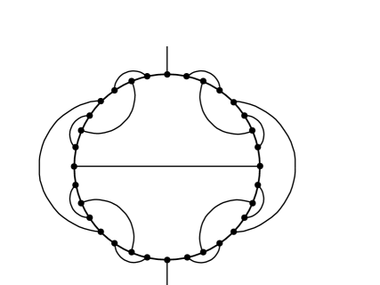
Figure 1: Depiction of the 3-regular network HN3 with a one-dimensional periodic backbone forming a ring, here with $k=5$. The top and bottom sites $n=0$ and $n=2^{k-1}$ require special treatment and are connected to external leads. With these connections, the entire network becomes 3-regular. Note that the graph is planar.

Previously (Boettcher et al., 2008), it was found that the average “chemical path” between sites on HN3 scales as

$$d^{HN3}\sim\sqrt{l}$$ (2)

with the distance $l$ along the backbone. In some ways, this property is reminiscent of a square-lattice consisting of $N$ lattice sites with diagonal $\sim\sqrt{N}$.

While the preceding networks are of a fixed, finite degree, we can extend HN3 in the following manner to obtain a new planar network of average degree 5, hence called HN5, at the price of a distribution in the degrees that is exponentially falling. In addition to the bonds in HN3, in HN5 we also connect all even sites to both of its nearest neighboring sites within the same level of the hierarchy $i>1$ in Eq. (1). The resulting network remains planar but now sites have a hierarchy-dependent degree, as shown in Fig. 2. To obtain the average degree, we observe that 1/2 of all sites have degree 3, 1/4 have degree 5, 1/8 have degree 7, and so on, leading to an exponentially falling degree distribution of ${\cal P}\left\{\alpha=2i+1\right\}\propto 2^{-i}$ for $i=1,\>2,\>3,\cdots$. Then, the total number of bonds $L$ in the (linear) system of size $N=2^{k}+1$ is

$$2L =2(2k-1)+ \sum_{i=1}^{k-1}\left(2i+1\right)2^{k-i}=5\times 2^{k}-4,$$ (3)

thus, the average degree is

$$\left\langle\alpha\right\rangle = \frac{2L}{N}\sim 5.$$ (4)

In HN5, the end-to-end distance is trivially 1, see Fig. 2. Therefore, we define as the diameter the largest of the shortest paths possible between any two sites, which are typically odd-index sites furthest away from long-distance bonds. For the $N=32$ site network depicted in Fig. 2, for instance, that diameter is 5 as measured between site 3 and 19 (0 is the left-most site), although there are many other such pairs. It is easy to show recursively that this diameter grows strictly as

$$d^{HN5} = 2\left\lfloor k/2\right\rfloor+1\sim\log_{2}N$$ (5)

with $\lfloor x\rfloor$ the integer portion of $x$. We have checked numerically that the average shortest path between any two sites also increases logarithmically with system size $N$.

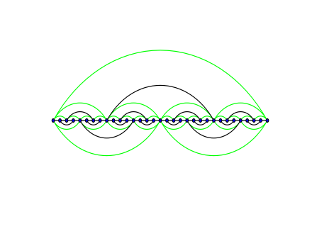
Figure 2: (Color online) Depiction of the planar network HN5. Black lines demark the original HN3 structure, the green-shaded lines are added to make HN5. Note that sites on the lowest level of the hierarchy have degree 3, then degree 5, 7, $\cdots$, making up a fraction of 1/2, 1/4, 1/8, $\cdots$, of all sites, thereby making for an average degree 5 of this network.

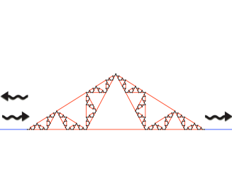
Figure 3: (Color online) Scattering a quantum electron off a linear version of HN3, here drawn as a branched Koch curve. The incoming electron on the left gets scattered into an outgoing transmitted portion (right) and reflected portion (left) on the attached external leads (blue-shaded). In this form of HN3, the one-dimensional backbone is marked by black links while the small-world links are shaded in red. Note, for instance, that the shortest end-to-end path here is the baseline of the Koch curve.

III Matrix RG for Hanoi Networks

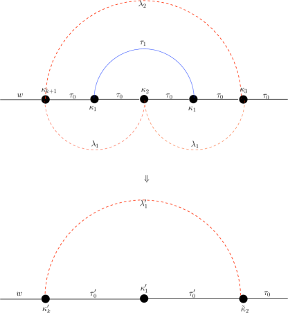
Figure 4: (Color online) Decimation of a block in the RG. The two sites with on-site energy $\kappa_{1}$ with a connecting bond of strength $\tau_{1}$ are decimated.

At each RG step, we decimate all the odd sites. Take site 0 to be at level $i=k+1$ in a linear geometry and at level $i=k$ in a ring geometry. As the odd sites each have only one small-world-type bond, we can divide the network into blocks containing 5 sites and decimate the pairs of two odd sites block by block. Let us start with the first block which contain sites 0,1,2,3 and 4. This decimation process for a linear geometry is shown in Fig. 4. Thus, here (see Appendix A) we have

$${\bf A}=\begin{pmatrix}\kappa_{k+1}&\lambda_{1}&\lambda_{2}\\ \lambda_{1}&\kappa_{2}&\lambda_{1}\\ \lambda_{2}&\lambda_{1}&\kappa_{3}\\ \end{pmatrix}$$ (6)

and

$${\bf D}=\begin{pmatrix}\kappa_{1}&\tau_{1}\\ \tau_{1}&\kappa_{1}\\ \end{pmatrix};\qquad{\bf B}=\begin{pmatrix}\tau_{0}&0\\ \tau_{0}&\tau_{0}\\ 0&\tau_{0}\\ \end{pmatrix}=\tau_{0}\begin{pmatrix}1&0\\ 1&1\\ 0&1\\ \end{pmatrix}.$$ (7)

After decimation,

$${\bf A^{\prime}}=\begin{pmatrix}\kappa^{\prime}_{k}&\tau^{\prime}_{0}&\lambda^{\prime}_{1}\\ \tau^{\prime}_{0}&\kappa^{\prime}_{1}&\tau^{\prime}_{0}\\ \lambda^{\prime}_{1}&\tau^{\prime}_{0}&\tilde{\kappa}_{2}\\ \end{pmatrix}={\bf A}-{\bf B}{\bf D}^{-1}{\bf B}^{\rm T}.$$ (8)

After simplification, we find that

$$\kappa^{\prime}_{k} = \kappa_{k+1}-\frac{\tau_{0}^{2}\kappa_{1}}{\kappa_{1}^{2}-\tau_{1}^{2}}$$ (9)

$$\kappa^{\prime}_{1} = \kappa_{2}-\frac{2\tau_{0}^{2}}{\kappa_{1}+\tau_{1}}$$ (10)

$$\tilde{\kappa}_{2} = \kappa_{3}-\frac{\tau_{0}^{2}\kappa_{1}}{\kappa_{1}^{2}-\tau_{1}^{2}}$$ (11)

$$\tau^{\prime}_{0} = \lambda_{1}-\frac{\tau_{0}^{2}}{\kappa_{1}+\tau_{1}}$$ (12)

$$\lambda^{\prime}_{1} = \lambda_{2}+\frac{\tau_{0}^{2}\tau_{1}}{\kappa_{1}^{2}-\tau_{1}^{2}}.$$ (13)

Here, the primed and unprimed quantities represent the $1$-st and the $0$-th level respectively in the RG recursion. Notice that the decimation of sites connected to site 4 [the right-most site in Fig. 4(a)] is not complete yet and therefore its on-site energy will be modified further when we decimate the odd sites of the next block which contain sites 4,5,6,7 and 8.

After the decimation of the next block we get

$$\kappa^{\prime}_{2} = \tilde{\kappa}_{2}-\frac{\tau_{0}^{2}\kappa_{1}}{\kappa_{1}^{2}-\tau_{1}^{2}}=\kappa_{3}-\frac{2\tau_{0}^{2}\kappa_{1}}{\kappa_{1}^{2}-\tau_{1}^{2}}.$$ (14)

Continuing the decimation block by block in this way, we find that

$$\kappa^{\prime}_{i} = \kappa_{i+1}-\frac{2\tau_{0}^{2}\kappa_{1}}{\kappa_{1}^{2}-\tau_{1}^{2}}\quad\textrm{for}\quad\forall i\in\{2,\ldots,k\}$$ (15)

$$\tau^{\prime}_{i} = \tau_{i+1}\quad\forall i\geq 1$$ (16)

$$\lambda^{\prime}_{i} = \lambda_{i+1}\quad\forall i\geq 2.$$ (17)

At first it appears that there are a lot of RG variables to worry about. However most of these RG variables are interdependent. It can be deduced from Eqs. (9,15, 16,17) that

$$\tau_{1}^{(m)} = \tau_{m+1}$$ (18)

$$\lambda_{2}^{(m)} = \lambda_{m+2},$$ (19)

and that the on-site energy parameter of the even sites is related to those of the odd sites as

$$\kappa_{i}^{(m)} = \kappa_{1}^{(m)}+\kappa_{m+i}-\kappa_{m+1}-2(\lambda_{1}^{(m)}-\lambda_{m+1})\quad\textrm{for}\quad\forall i\in\{2,\ldots,k-m\}$$ (20)

and that specifically for a linear geometry, the on-site energy parameter of the end sites

$$\kappa_{k+1-m}^{(m)} = \kappa_{k+1}+(\kappa_{2}^{(m)}-\kappa_{m+2})/2\quad\textrm{for}\quad\forall m\in\{0,\ldots,k-2\}.$$ (21)

Thus we are left with just three independent RG variables which are $\kappa_{1}^{(m)}$, $\tau_{0}^{(m)}$ and $\lambda_{1}^{(m)}$ governed by the RG equations

$$\kappa_{1}^{(m+1)}\>=\>\kappa_{1}^{(m)}+\kappa_{m+2}-\kappa_{m+1}-2(\lambda_{1}^{(m)}-\lambda_{m+1})-\frac{2[\tau_{0}^{(m)}]^{2}}{\kappa_{1}^{(m)}+\tau_{m+1}}\quad \forall m\in\{0,\ldots,k-2\}$$ (22)

$$\tau_{0}^{(m+1)}\>=\>\lambda_{1}^{(m)}-\frac{[\tau_{0}^{(m)}]^{2}}{\kappa_{1}^{(m)}+\tau_{m+1}}\quad \forall m\in\{0,\ldots,k-1\}$$ (23)

$$\lambda_{1}^{(m+1)}\>=\>\lambda_{m+2}+\frac{[\tau_{0}^{(m)}]^{2}\tau_{m+1}}{[\kappa_{1}^{(m)}]^{2}-\tau_{m+1}^{2}}\quad \forall m\in\{0,\ldots,k-1\}.$$ (24)

IV Analysis of the RG Equations

IV.1 One-dimensional Lattice (HN2)

It will prove helpful to demonstrate the general set of recursions [Eqs. (22, 23, 24)] by way of the one-dimensional ($d=1$) ring of $N=2^{k}$ sites. For consistency we call this the HN2 network, or Hanoi network with 2 bonds per site (with additional bonds for the input/output leads in the ring geometry). We can employ the recursions to explore the transmission through a $d=1$ ring of $N=2^{k}$ sites. The energy scale chosen throughout is such that the (uniform) transmissivity for each bond has a unit weight. With that, we obtain the initial conditions

$$\kappa_{i}^{(0)} = E,\qquad(i\geq 1),$$

$$\tau_{0}^{(0)} = -1,$$ (25)

$$\tau_{i}^{(0)} = 0,\qquad(i\geq 1),$$

$$\lambda_{i}^{(0)} = 0,\qquad(i\geq 1)\>.$$

Eqs. (22, 23, 24) simplify to

$$\kappa_{m+1} = \kappa_{m}-\frac{2\tau_{m}^{2}}{\kappa_{m}},$$ (26)

$$\tau_{m+1} = -\frac{\tau_{m}^{2}}{\kappa_{m}},$$

where $\kappa_{m}\equiv\kappa_{i}^{(m)}$ and $\tau_{i}=\lambda_{i}\equiv 0$ for all $i\geq 1$ and $\tau_{m}\equiv\tau_{0}^{(m)}$. These nonlinear recursions are easily solved by defining $s_{m}=-\kappa_{m}/\tau_{m}$ for which $s_{m+1}=s_{m}^{2}-2$, obtained by dividing the $2^{\rm nd}$ by the $3^{\rm rd}$ line in Eqs. (26). Formally, the solution is

$$s_{m}=2\cos\left[2^{m}\arccos\left(\frac{\kappa^{(0)}}{2\tau^{(0)}}\right)\right]=2T_{2^{m}}\left(\frac{\kappa^{(0)}}{2\tau^{(0)}}\right),$$ (27)

where $T_{n}(x)$ refers to the $n$-th Chebyshev polynomial of the first kind (Abramowitz and Stegun, 1964). Inserting into Eqs. (26) and applying the initial conditions in Eqs. (25), generates the results

$$\tau^{(m)} = -\prod_{i=0}^{m-1}\frac{1}{s_{i}},$$

$$\kappa^{(m)} = s_{m}\prod_{i=0}^{m-1}\frac{1}{s_{i}},$$ (28)

where the last equality emerges under reordering factors in the products.

Eq. (69) in Appendix B shows that the transmission amplitude $t$ is directly proportional to $\tau^{(k)}$. Clearly, if there is no transmission on any bond, i.e. $\tau^{(k)}=0$, for a given input energy $E$, there can be no transmission through the network itself, no matter what happens on the sites. But instead of plotting $\tau^{(k)}$, it will prove more instructive to plot $\kappa^{(k)}$. It is easy to see from Eqs. (28) that $\kappa^{(k)}$ varies rapidly whenever $\tau^{(k)}$ does, but that $\kappa^{(k)}$ varies smoothly whenever $\tau^{(k)}$ vanishes. In the following, we will see that this behavior remains true for HN3 and HN5, in which case the variation of $\kappa^{(k)}$ with $\kappa^{(0)}=E$ provides more information beyond the mere vanishing of $\tau^{(k)}$.

We have evolved the RG-recursion in (26) for the initial conditions in (25) and plotted $\kappa^{(k=10)}$ as a function of $\kappa^{(0)}=E$ in Fig. 5. Even at that system size, $N=2^{k}=1024$, delocalized states completely cover the domain $-2\leq E\leq 2$.

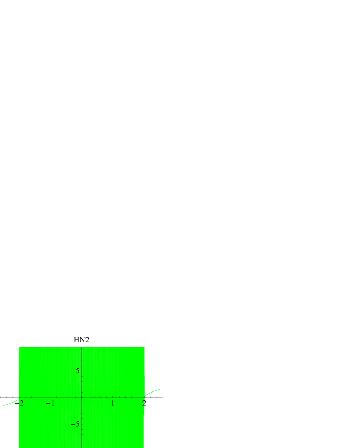
Figure 5: (Color online) Plot of $\kappa^{(10)}$ in Eq. (26) as a function of its initial condition $\kappa^{(0)}=E$. Even at this small order, the function varies extremely rapidly, such that its (green-shaded) line completely covers the shown domain. Thus, for $-2\leq E\leq 2$, $\kappa^{(m)}$ for any sufficiently large $m$ is a random function. Correspondingly, the transmission spectrum is dense, with full transmission close to any input energy $E$ such that particles do not localize.

IV.2 Case HN3

Again, we can employ the RG Eqs. (22, 23, 24) for transmission through HN3 consisting of a ring of $N=2^{k}$ sites, as in Fig. 1. Since all initial diagonal entries are identical, the hierarchy for the $\kappa_{i}$ collapses and we retain only two nontrivial relations, one for $\kappa_{1}$ and one for all other $\kappa_{i}\equiv\kappa_{2}$ for all $i\geq 2$. Here, all $\tau_{i}$ are non-zero, encompassing the backbone links ($i=0$) and all levels of long-range links ($i\geq 1$). But it remains $\tau_{i}\equiv-1$ for $i\geq 1$ at any step $m$ of the RG, in particular, $\tau_{1}^{(m)}\equiv-1$ throughout; only the backbone $\tau_{0}$ renormalizes non-trivially. Although all links of type $\lambda_{i}$ are initially absent in this network, the details of the RG calculation shows that under renormalization terms of type $\lambda_{1}$ emerge while those for $\lambda_{i}$ for $i\geq 2$ remain zero at any step. Thus, we obtain far more elaborate RG recursion equations compared to those of HN2. Abbreviating $\kappa_{m}\equiv\kappa_{1}^{(m)}$, $\tau_{m}\equiv\tau_{0}^{(m)}$, and $\lambda_{m}=\lambda_{1}^{(m)}$, Eqs. (22, 23, 24) and their initial conditions reduce to

$$\begin{matrix}\kappa_{m+1}&=&\kappa_{m}-2\lambda_{m}-\frac{2\tau_{m}^{2}}{\kappa_{m}-1},&\qquad&(\kappa_{0}=E),\\ \tau_{m+1}&=&\lambda_{m}-\frac{\tau_{m}^{2}}{\kappa_{m}-1},&\qquad&(\tau_{0}=-1),\\ \lambda_{m+1}&=&-\frac{\tau_{m}^{2}}{\kappa_{m}^{2}-1},&\qquad&(\lambda_{0}=0).\\ \end{matrix}$$ (29)

We have evolved the RG-recursion in (29) and plotted $\kappa_{k=200}$ as a function of $\kappa_{0}=E$ in Fig. 6. Even at that enormous (and definitely asymptotic) system size, $N=2^{200}\approx 10^{70}$, domains of localized states remain asymptotically inside the physically relevant domain of $-2\leq E\leq 2$. For comparison, the radius of the visible universe is only about $10^{40}$ fm.

In the next subsection, we will explore the asymptotic properties of these recursions for large $m$. We will find domains in $E$ of stationary solutions, which are particular for HN3, and show that the special points where this analysis fails correspond to transitions between localized and delocalized behavior.

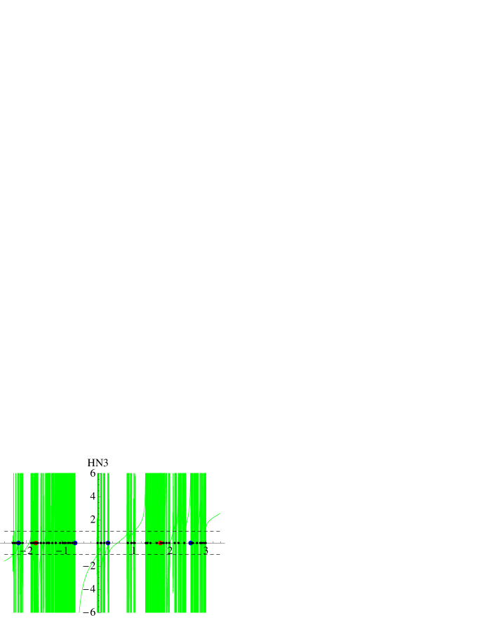
Figure 6: (Color online) Plot of $\kappa_{200}$ in Eq. (29) as a function of its initial condition $\kappa_{0}=E$. Bands of localized and delocalized states intermix. Correspondingly, there are localization-delocalization transitions already before the addition of any additional randomness in HN3, merely as a function of the input energy $E$. On the horizontal axis, we have marked the solutions $E_{s}^{(i)}$ of Eq. (36) for $s=1$ (red dots), $s=2$ (blue dots), and $s=6$ (small black dots). The accumulation of the latter demonstrates (even for such a small value of $s$) that the band gaps are associated with the absence of such solutions. While the solutions for $s=1$ happen to be interior to the bands, some of those for $s=2$ appear to mark the band edges, in particular the one at $E=E_{2}^{(2)}=-0.637875$.

IV.2.1 Analysis of the Steady State:

We can analyze the absorbing steady state, which is the unique feature of HN3 (in contrast to HN2 and HN5) leading to band gaps, as follows. Numerical trails show that the RG recursions in Eq. (29) reach a steady state for certain initial conditions $E$ when for all $m$ larger than some $m_{0}$ it is

$$1 \gg \lambda_{m}\gg\frac{\tau_{m}^{2}}{\kappa_{m}-1},\qquad(m\to\infty).$$ (30)

The leading contribution for $\kappa_{m}$ in Eq. (29) then suggests

$$\kappa_{m+1} \sim \kappa_{m}\sim\kappa_{\infty},$$ (31)

which is a constant that is difficult to derive from the initial conditions, $\kappa_{0}=E$, unfortunately.

From the recursion for $\tau_{m}$ in Eq. (29), we further obtain

$$\tau_{m+1} \sim \lambda_{m}\sim-\frac{\tau_{m-1}^{2}}{\kappa_{\infty}^{2}-1}.$$ (32)

This 2nd order difference equation has two solutions, of which we discard the oscillatory one, to get for large $m>m_{0}$:

$$\tau_{m} \sim -\left(\kappa_{\infty}^{2}-1\right)\exp\left\{-C\sqrt{2^{m}}\right\},$$

$$\lambda_{m} \sim -\left(\kappa_{\infty}^{2}-1\right)\exp\left\{-C\sqrt{2^{m+1}}\right\},$$

where $C>0$ is another undetermined constant that depends on $E$. Using the recursion for $\kappa_{m}$ in Eq. (29) to next-to-leading order yields

$$\kappa_{m+1} \sim \kappa_{m}-2\lambda_{m},$$ (33)

$$\sim \kappa_{m}+2\left(\kappa_{\infty}^{2}-1\right)\exp\left\{-C\sqrt{2^{m+1}}\right\},$$ (34)

which, when summed from a $m>m_{0}$ to $\infty$ results in

$$\kappa_{m} \sim \kappa_{\infty}-2\left(\kappa_{\infty}^{2}-1\right)\exp\left\{-C\sqrt{2^{m+1}}\right\},$$ (35)

where we have kept only the first term in the sum, as the summand is exponentially decaying.

The consequences of this analysis are quite dramatic. If such a steady-state solution is reached, both transmission rates $\tau$ and $\lambda$ vanish, only leaving a finite on-site energy $\kappa_{\infty}$. Hence, there can not be any transmission through the network when such a state is reached, and gaps emerge in the transmission spectrum. Since the system size is given by $N=2^{m}$, this result implies that finite size corrections scale with $\exp\left\{-C\sqrt{2N}\right\}$, i.e. finite-size corrections decay rapidly with a stretched exponential. Note that there are no steady-state solutions that cross $\kappa_{\infty}=\pm 1$ (dashed lines in Fig. 6), where the correction in Eq. (35) would break down. Instead, the approach of $\kappa_{\infty}\to\pm 1$ frequently appears to be associated with the emergence of a band edge between localized and delocalized states.

IV.2.2 Band-Edge Analysis:

The non-trivial band structure warrants some further investigation. In particular, we can associate such band edges with initial conditions $E=E_{s}^{(i)}$ for which there exists a $m=s$ such that

$$\kappa_{s}\left(E_{s}^{(i)}\right) = -1,$$ (36)

a singular point in the recursion for $\lambda_{s+1}$. [Interestingly, any singularity at $\kappa_{m}=+1$ appears to be benign in that it does not affect the continuity in $\kappa_{m}$ as a function of $E$ for $m\to\infty$; it afflicts each quantity in Eqs. (29) simultaneously, leading to a divergence in $\kappa_{m+1}$, $\tau_{m+1}$, and $\lambda_{m+1}$ just so that $\kappa_{m+2}\approx\kappa_{m-1}$, $\tau_{m+2}\approx\tau_{m-1}$, $\lambda_{m+2}\approx\lambda_{m-1}$.] In Fig. 6, we have also marked the real solutions $E_{s}^{(i)}$ of Eq. (36) for $s=1$, 2, and 6. Clearly, those solutions strongly correlate with the bands, and there appear to be none within the gaps (although we have not been able to prove this conjecture). But while those solutions for $s=1$, $E_{1}^{(1,2)}=\pm\sqrt{3}$, are located well within some band (as are those for $s=6$), the four real solutions of Eq. (36) for $s=2$ satisfy the quartic equation

$$0 = 1-2E-6E^{2}+E^{4}$$ (37)

and appear to be all associated with some more or less significant band edge, see blue dots in Fig. 6. We can speculate that there is a whole hierarchy of transitions, each associated with one of the solutions $E_{m}^{(i)}$, which may become dense on certain intervals. While we don’t know what determines those intervals precisely, we can analyze the behavior in the neighborhood of Eq. (36). We observed that the recursions in Eq. (29) possess stable steady-state solutions for large $m$ characterized by $\tau_{m}\sim\lambda_{m}\to 0$, i.e. vanishing bond-strength between input and output. These solutions prevail in the observed band gaps, which accordingly correspond to localized states. It seems that the reason for the persistence of gaps derives from that stability: band gaps emerge whenever the steady state is reached before Eq. (36) can be satisfied. For instance, in the case of HN5 below, any putative steady-state solution proves unstable for sufficiently large $m$ such that any band gaps are transitory only, see Fig. 9.

For the analysis of the recursion Eq. (29), we assume that for some $m=s$, we reach

$$\kappa_{s} \sim -1+\epsilon,\qquad(\epsilon\ll 1),$$ (38)

where $\epsilon=\epsilon(E)$ may be of either sign, depending on $\Delta E=E-E_{s}^{(i)}$. Generically, $\epsilon\propto\Delta E$, see Sec. IV.2.3 below. Assuming that $\tau_{s},\lambda_{s}\ll 1/\epsilon$ leads to

$$\kappa_{s+1} \sim -1-2\lambda_{s}+\tau_{s}^{2}+O(\epsilon),$$

$$\tau_{s+1} \sim \lambda_{s}+\frac{\tau_{s}^{2}}{2}+O(\epsilon),$$ (39)

$$\lambda_{s+1} \sim \frac{\tau_{s}^{2}}{2\epsilon}+\frac{\tau_{s}^{2}}{4}+O(\epsilon),$$

which leaves only $\lambda_{s+1}$ singular. After one more recursion step, we get instead

$$\kappa_{s+2} \sim -\frac{\tau_{s}^{2}}{\epsilon}+\frac{2+6\lambda_{s}+2\lambda_{s}^{2}-2\tau_{s}^{2}-5\lambda_{s}\tau_{s}^{2}}{-2-2\lambda_{s}+\tau_{s}^{2}}+O(\epsilon),$$

$$\tau_{s+2} \sim \frac{\tau_{s}^{2}}{2\epsilon}+\frac{2\lambda_{s}^{2}+\tau_{s}^{2}+3\lambda_{s}\tau_{s}^{2}}{4+4\lambda_{s}-2\tau_{s}^{2}}+O(\epsilon),$$ (40)

$$\lambda_{s+2} \sim O(1).$$

At this point, Eq. (29) decouple to leading order, as $\lambda_{s+2+i+1}\sim-\tau_{s+2+i}^{2}/\kappa_{s+2+i}^{2}\sim-1/4$ remains of order $O(1)$ while both $\kappa_{s+2+i}$ and $\tau_{s+2+i}$ are of order $O(1/\epsilon)$, and we get for some $i\geq 0$

$$\kappa_{s+2+i+1} \sim \kappa_{s+2+i}-\frac{2\tau_{s+2+i}^{2}}{\kappa_{s+2+i}},$$

$$\tau_{s+2+i+1} \sim -\frac{\tau_{s+2+i}^{2}}{\kappa_{s+2+i}}.$$ (41)

These are exactly the same recursions we obtained in Eq. (26) for HN2, with the solution in Eq. (27):

$$\frac{\kappa_{s+2+i}}{2\tau_{s+2+i}} \sim -T_{2^{i}}\left(-\frac{\kappa_{s+2}}{2\tau_{s+2}}\right),$$ (42)

where from Eq. (40) we have

$$\frac{\kappa_{s+2}}{2\tau_{s+2}} \sim -1+A\frac{\epsilon}{\tau_{s}^{2}},$$ (43)

$$A = \frac{2+6\lambda_{s}-3\tau_{s}^{2}-8\lambda_{s}\tau_{s}^{2}}{2+2\lambda_{s}-\tau_{s}^{2}}\>.$$ (44)

With that inserted into Eq. (42), we can deduce

$$\frac{\kappa_{s+2+i}}{2\tau_{s+2+i}} \sim -T_{2^{i}}\left(1-A\frac{\epsilon}{\tau_{s}^{2}}\right),$$ (45)

$$\sim 1-A\frac{\epsilon}{\tau_{s}^{2}}T_{2^{I}}^{\prime}\left(1\right),$$

$$\sim 1-2^{2i}A\frac{\epsilon}{\tau_{s}^{2}},$$

since $T^{\prime}_{n}(x)=nU_{n-1}(x)$ and $U_{n-1}(1)=n$, referring to the Chebyshev polynomial of the 2nd kind, $U_{n}(x)$ (Abramowitz and Stegun, 1964). With the exponential growth in $i$ of the correction amplitude in the asymptotic expansion in Eq. (45), the expansion breaks down at some $i\sim i_{0}$ such that the correction itself becomes of $O(1)$, i.e.

$$i_{0} \sim \frac{1}{2}\log_{2}\left(\frac{\tau_{s}^{2}}{\left|A\epsilon\right|}\right).$$ (46)

For $i>i_{0}$, according to the first line of Eq. (45) the ratio $\kappa_{s+2+i}/\tau_{s+2+i}$ either rises or falls exponentially, depending on whether $A\epsilon<0$ or $A\epsilon>0$, respectively. In the latter case, $\kappa$ becomes less relevant and the bonds $\tau$ and $\lambda$ determine the future evolution in $m$, leading again to the chaotic behavior in $\kappa_{m}$ observed within the bands in Fig. 6. On the other hand, if $A\epsilon>0$, the on-site energies $\kappa$ dominate exponentially over the couplings $\tau$ and $\lambda$, evolving towards an absorbing steady state on the band-gap side of the transition.

IV.2.3 Scaling Relation for $\kappa_{\infty}(E)$:

As mentioned in Sec. IV.2.1, we can not generally predict the dependence of the asymptotic behavior on the initial condition $E$. But we can use the analysis of that section at least to determine the behavior of $\kappa_{\infty}(E)$ on the approach to those band edges where it diverges.

It is easy to show, using just the singular terms for $\kappa$ and $\tau$ in Eq. (40) inserted into the recursions in Eq. (41), that both simultaneously decay exponentially with $i$ at least while $i\lesssim i_{0}$ from Eq. (46),

$$\kappa_{s+2+i} \sim -\frac{\tau_{s}^{2}}{2^{i}\epsilon}+O(1),$$ (47)

$$\tau_{s+2+i} \sim \frac{\tau_{s}^{2}}{2^{i+1}\epsilon}+O(1).$$

At $i\sim i_{0}$ there is a cross-over beyond which for all $i>i_{0}$ it is $\tau_{s+2+i}\to 0$ and a saturated value of $\kappa_{s+2+i}\to\kappa_{\infty}$ is reached. We can obtain the dominant asymptotic behavior at the cross-over from

$$\kappa_{\infty} \sim \kappa_{s+2+i_{0}}\sim-\frac{\tau_{s}^{2}}{\epsilon\sqrt{\frac{\tau_{s}^{2}}{\left|A\epsilon\right|}}},$$ (48)

$$\sim -\sqrt{\left|A\right|\tau_{s}^{2}}\frac{\mathrm{sgn}\left(\epsilon\right)}{\left|\epsilon\right|^{\frac{1}{2}}}.$$

We can further establish a (generic) relation between $\epsilon$ and

$$\Delta E \sim E-E_{s}^{(i)}$$

by extending the discussion of Eq. (36) in Sec. IV.2.2. We set

$$-1+\epsilon\left(\Delta E\right) \sim \kappa_{s}\left(E_{s}^{(i)}+\Delta E\right),$$

$$\sim \kappa_{s}\left(E_{s}^{(i)}\right)+\kappa^{\prime}_{s}\left(E_{s}^{(i)}\right)\Delta E,$$

$$\sim -1+\kappa^{\prime}_{s}\left(E_{s}^{(i)}\right)\Delta E,$$

since $\kappa_{s}\to-1$ is a regular limit for $\Delta E\to 0$, as Eq. (37), for example, suggests. Hence,

$$\epsilon\left(\Delta E\right) \sim \kappa^{\prime}_{s}\left(E_{s}^{(i)}\right)\Delta E,$$

and we conclude

$$\kappa_{\infty} \sim -\sqrt{\frac{\left|A\right|\tau_{s}^{2}}{\left|\kappa^{\prime}_{s}\left(E_{s}^{(i)}\right)\right|}}\frac{\mathrm{sgn}\left(\kappa^{\prime}_{s}\left(E_{s}^{(i)}\right)\Delta E\right)}{\left|\Delta E\right|^{\frac{1}{2}}}$$ (49)

with $\Delta E\to 0$. In Fig. 7 we have tested the asymptotic relation $1/\kappa_{\infty}\sim\sqrt{\left|\Delta E\right|}$ in the band gap near $E_{s}^{(2)}=-0.637875\ldots$, a solution of Eq. (37) marked blue in Fig. 6.

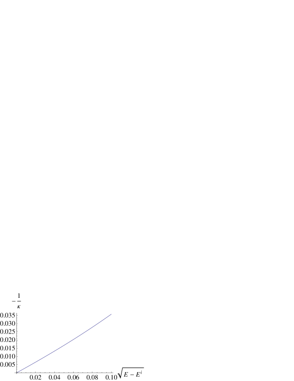
Figure 7: (Color online) Plot of $1/\kappa_{\infty}$ as a function of $\sqrt{E-E_{s}^{(i)}}$ for $E\to E_{s}^{(i)}$ to test Eq. (49). Here, $E_{2}^{(2)}=-0.637875$, marked as the 2nd blue dot from the left in Fig. 6.

IV.3 Interpolation between HN2 and HN3

It proves fruitful to consider an interpolation between the case of HN2 in Sec. IV.1 and HN3 in Sec. IV.2 in terms of a one-parameter family of models. To wit, we can accomplish such an interpolation by weighting the transmission along the small-world links (see red-shaded links in Fig. 3) by a factor of $y$ relative to that of the backbone links (see black links in Fig. 3). Clearly, more generally, hierarchy and/or distance-dependent weights could be introduced as well. For $y=0$, small-world links are non-existent, and we have the linear lattice HN2. Although still mostly delocalized, the states of the systems immediately change behavior when $y>0$, and we find localized states which expand their domain towards $y=1$, corresponding to HN3, and continue to do so until at about $y=4$ no transmission is possible any longer: The more we weight small-world links here, which classically would expedite transport (Otwinowski and Boettcher, 2009), the less quantum transport is possible! In the next section we will see that even more small-world links, as in HN5, can lead to more transmission again. Hence, the detailed structure of the links matter.

To explore this $y$-family of models, we have to generalize Eq. (29) appropriately:

$$\begin{matrix}\kappa_{m+1}&=&\kappa_{m}-2\lambda_{m}-\frac{2\tau_{m}^{2}}{\kappa_{m}-y},&\qquad&(\kappa_{0}=E),\\ \tau_{m+1}&=&\lambda_{m}-\frac{\tau_{m}^{2}}{\kappa_{m}-y},&\qquad&(\tau_{0}=-1),\\ \lambda_{m+1}&=&-\frac{y\,\tau_{m}^{2}}{\kappa_{m}^{2}-y^{2}},&\qquad&(\lambda_{0}=0),\end{matrix}$$ (50)

since for all non-backbone links in Eqs. (22, 23, 24) it is $\tau_{i\geq 1}^{(0)}=y\,\tau_{0}^{(0)}$, i.e. $\tau_{i\geq 1}^{(m)}=-y$ at every RG-step. Note that these equations reduce to Eqs. (26) for $y=0$ (with all $\lambda_{i}\equiv 0$) and to Eq. (29) for $y=1$.

In Fig. 8 we map out the state of Eq. (50) after the $1000^{\rm th}$ iteration based on whether a steady state has been reached or not, depending on the incoming energy $E$ and the relative weight $y$. For any $y>0$, the ability to transmit has a strong chaotic dependence on these parameters, and ceases completely for $y>4$. Even within domains of apparent transmission there are often sub-domains where no transmission is possible, and it is not clear whether true conduction bands exist. Since in this model the long-range links are not connected to each other except through the backbone, one may speculate that even at high weight these links merely lead to localized resonances that interfere with transport along the backbone instead of conveying it. (A similar confinement effect was observed for the RG applied to random walks on HN3 in Ref. (Boettcher and Goncalves, 2008).)

It is straightforward to generalize the discussion for HN3 in Sec. IV.2 to this model. In particular, for the band-edge analysis we have to generalize Eq. (36) to read

$$\kappa_{s}\left(E_{s}^{(i)}\right) = -y.$$ (51)

For $s=0,1,2$, and 3, the numerical solutions $E_{s}^{(i)}(y)$ are also plotted as lines in Fig. 8. The result underlines the contention made before for HN3 that the transitions between transmission and localization are closely associated with these singular points of the Eq. (50). For instance, the big blue-shaded dots in Fig. 6 correspond here to the intersection of the simple-dashed line for $s=2$ with the dotted horizontal line along $y=1$ (i. e. HN3). Dominant features emerge, such as the line $\kappa_{0}=E=-y$. Other interesting points become apparent, for instance, the one at $y=-E=1/\sqrt{2}$. While there is otherwise no apparent relation to solutions of $\kappa_{s}=+y$, it should be noted that its $s=0$ case does produce a distinct feature in the line $E=y$.

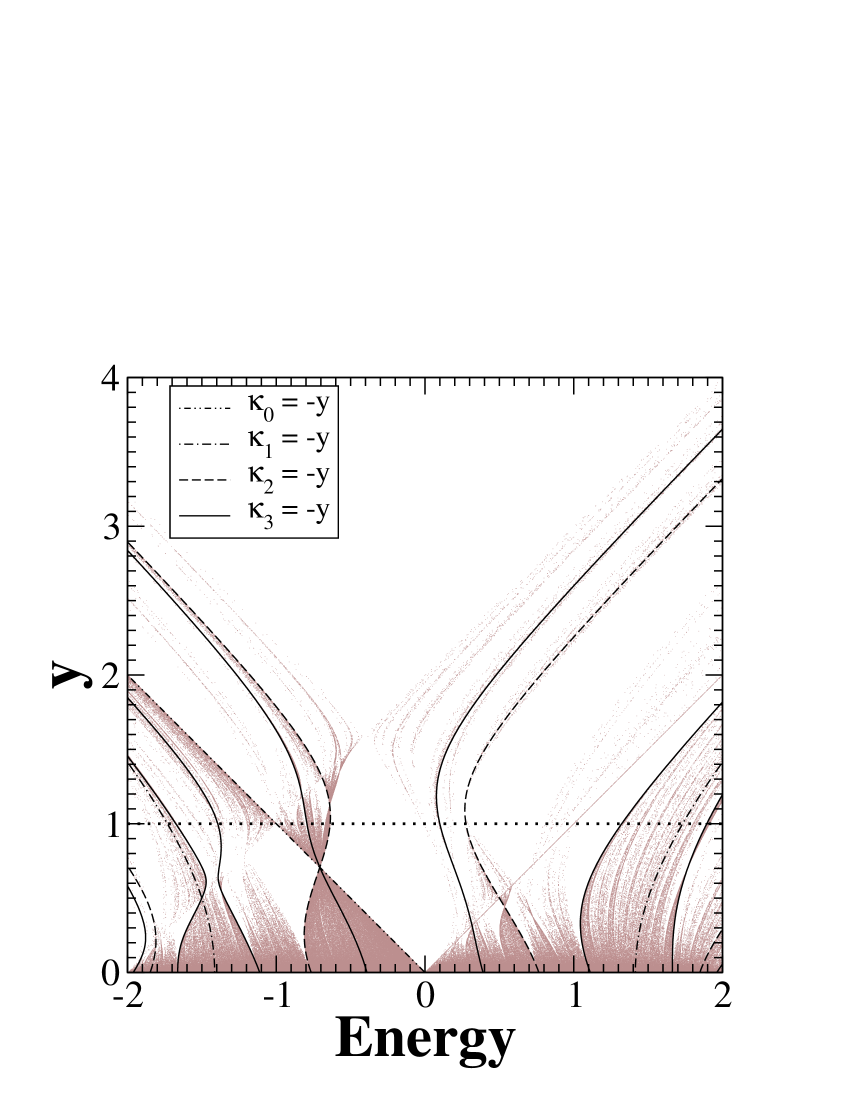
Figure 8: (Color online) Plot of the state of Eq. (50) after 1000 iterations for initial energies $\kappa_{0}=E$ and the interpolation parameter $y$ (the resolution is 0.001 in each direction). Shaded points have not, or not yet, converged to a steady-state, i.e. those values possess non-zero transmission. At $y=0$, corresponding to HN2, the system transmits for any input energy, $-2\leq E\leq 2$. As soon as $y>0$, bands of localized states emerge (especially at $E=0$), and the remaining transmitting states exhibit a chaotic dependence on the parameters. At $y=1$, the case of HN3 marked by a dotted horizontal line, only a few non-localized states remain, and the further strengthening of small-world links diminish transmission even more, such that it ceases completely for $y>4$. Any band of transmitting states appears to be accompanied by solutions of Eq. (51), which here are draw as curves for the lowest orders of the recursion only; $s=0,1,2,$ and 3 corresponding respectively to dot-dot-dashed, dot-dashed, dashed, and solid curves.

IV.4 Case HN5

In close correspondence with the treatment in Sec. IV.2, we can employ the RG in Eqs. (22, 23, 24) for transmission through HN5 consisting of a ring of $N=2^{k}$ sites. The sole difference with Sec. IV.2 is that all links of type $\lambda_{i}$ are initially present in this network. Yet, the details of the RG calculation in Sec. III show that under renormalization only links of type $\lambda_{1}$ renormalize while those $\lambda_{i}$ for $i\geq 2$ remain unrenormalized at any step. The diagonal elements are again hierarchy-independent, $\kappa_{i}^{(0)}\equiv E$, while the recursion for $\lambda$ changes. Abbreviating $\kappa\equiv\kappa_{1}$, $\tau\equiv\tau_{0}$, and $\lambda=\lambda_{1}$, Eqs. (22, 23, 24) and their initial conditions reduce to

$$\begin{matrix}\kappa_{m+1}&=&\kappa_{m}-2\lambda_{m}-2-2\frac{\tau_{m}^{2}}{\kappa_{m}-1},&\qquad&(\kappa_{0}=E),\\ \tau_{m+1}&=&\lambda_{m}-\frac{\tau_{m}^{2}}{\kappa_{m}-1},&\qquad&(\tau_{0}=-1),\\ \lambda_{m+1}&=&1-\frac{\tau_{m}^{2}}{\kappa_{m}^{2}-1},&\qquad&(\lambda_{0}=-1).\end{matrix}$$ (52)

We have evolved the RG-recursion in Eq. (52) and plotted $\kappa^{(k=10)}$ as a function of $\kappa^{(0)}=E$ in Fig. 9. At that (definitely not asymptotic) system size, $N=2^{10}\approx 10^{3}$, domains of localized states remain which will disappear asymptotically, as for the case of HN2 in Fig. 5. Unlike for HN3, there are no steady-state solutions for Eq. (52) that could signal localization. It is interesting to analyze the cause of this behavior. Since the $\lambda$-links [green-shaded in Fig. 2] are an original feature of the network, the RG recursion in Eq. (52) for $\lambda_{m}$ obtain a constant offset preventing $\lambda_{m}$, and hence $\tau_{m}$, from vanishing. Unlike for HN3, these small-world links allow perpetual transmission within a given level of the hierarchy, instead of interfering with other paths, and transmission is enhanced. In fact, we have studied also an interpolation between HN3 and HN5 by attaching a relative weight $y$ to these $\lambda$-links in HN5, relative to the otherwise uniform links present in HN3. Thus, for $y=0$ HN3 is obtained, and for $y=1$ we get HN5. Yet, we find that for any $y>0$, this model eventually behaves like HN5, with unfettered transmission throughout the energy spectrum.

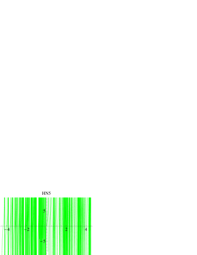
Figure 9: (Color online) Plot of $\kappa^{(10)}$ in Eqs. (52) for HN5 as a function of its initial condition $\kappa^{(0)}=E$. Bands of localized and delocalized states intermix, but those localized intervals disappear asymptotically.

V Summary and Discussion

We have devised a decimation RG procedure within the matrix methodology of Ref. (daboul, ) to obtain transmission of quantum electrons through networks within the tight-binding model approximation. This decimation RG procedure of Appendix A can in principle be implemented for any network, in that Eq. (53) with $n+m$ sites is reduced to Eq. (59) with $n$ sites. For general networks the bookkeeping required could become prohibitive. However, we find the RG equations well suited to the networks we have chosen to analyze, namely the hierarchical networks called HN3 (Hanoi Network with 3 bonds per site) and HN5 (Hanoi Network with an average of 5 bonds per site). This is because the RG can proceed block-wise, as depicted in Fig. 4. We have analyzed both the ring geometry (Fig. 1) and the linear geometry (Figs. 1 and 3) of these networks, with the only difference being the last steps of the RG (Appendix B). We have also analyzed how the transmission for the linear lattice (which we label HN2) changes with the strength of the small-world-type bonds added to form HN3 (Fig. 8).

The Hanoi networks are hierarchical models that provide an intermediary between regular lattices and lattices that have random small-world bonds placed on regular lattices. Since the small-world-type bonds in the Hanoi networks provide short-cuts between sites, one might expect intuitively that they should provide extra paths for transmission. However, because of the hierarchical nature of the networks, the networks no longer possess translational symmetry. This broken symmetry is seen by the incoming quantum electrons, and can lead to Anderson-type localization. For the HN3 network with variable strength $y$ for the small-world-type bonds, we find that the more we weight the small-world links, which classically would expedite transport (Otwinowski and Boettcher, 2009), the less quantum transport is possible (Fig. 8). Furthermore, we find that HN3 has band edges at particular energies $E$ of the incoming electrons, between band gaps with near zero transmission and regions of extended wavefunctions and transmission near unity. The network HN5 adds still more small-world type bonds to HN3, but we find that for any non-zero strength of these additional bonds the band edges seen in HN3 disappear and approximately unfettered transmission is seen for large enough lattices for any energy of the incoming electrons. Thus the hierarchical nature of these lattices lead to very interesting transmission properties. Thus for these hierarchical lattices, the metal-insulator transitions depend on quantities other than just the embedding dimension. Similar effects have been seen for critical phenomena in hierarchical lattices, but only where translational symmetry is broken Gefen1980 ; Banav1983 ; LeGuillou1987 ; Novotny1992 ; Novotny1993 .

Since the HN3 and HN5 networks are planar (see for example Fig. 3), experimental realizations of these networks should be possible to construct using etching techniques. These experiments would lead to very interesting device physics, in particular at the energy-dependent band edges we have analyzed for HN3.

Appendix A General Matrix Formulation of the RG

As in Ref. (daboul, ), a ‘blob’ of atoms in the tight-binding approximation is considered to be connected to two semi-infinite leads. Each semi-infinite lead is considered to be a linear arrangement of tight-binding sites with on-site energy $0$ and a hopping parameter of $-1$ (setting the energy scale). The incoming (outgoing) lead is connected to the ‘blob’ sites by a vector of hopping parameters ${\vec{w}}$, (respectively, ${\vec{u}}$). The Schrödinger equation for the infinite system, ${\cal H}_{\infty}{\vec{\Psi}}=E{\vec{\Psi}}$ must be solved with the appropriate boundary conditions. The ansatz made daboul is that the wavefunction at every site in the in-coming lead has the form $\psi_{m-1}=e^{imq}+re^{-imq}$ with $m=-\infty,\cdots,-2,-1,0$, and the outgoing lead has the wavefunction $\psi_{m+1}=te^{imq}$ with $m=0,1,2,\cdots,\infty$. The wavevector $q$ is related to the energy of the incoming electron by $E=2\cos(q)$. The reflection probability is $R=|r|^{2}$ and the transmission probability is $T=|t|^{2}$. With this ansatz, the required solution of the infinite matrix Schödinger equation reduces to the solution of a finite matrix equation of dimension two larger than then number of sites in the ‘blob’. Unlike Ref. (daboul, ), we assume no direct hopping between the leads, i.e. no short-cut path around the ‘blob’.

Consider the case with $n+m$ sites in the blob. We specialize to the case where all hopping parameters ($\tau$ or $\lambda$) and on-site energies (convoluted with $E$ to give $\kappa$) are real. The $(n+m+2)\times(n+m+2)$ matrix to solve for the transmission $T=|t|^{2}$ is daboul

$$\begin{pmatrix}\xi&{\vec{w}}^{\rm T}&{\vec{w}}_{d}^{\rm T}&0\\ {\vec{w}}&{\bf A}&{\bf B}&{\vec{u}}\\ {\vec{w}}_{d}&{\bf B}^{\rm T}&{\bf D}&{\vec{u}}_{d}\\ 0&{\vec{u}}^{\rm T}&{\vec{u}}_{d}^{\rm T}&\xi\\ \end{pmatrix}\begin{pmatrix}1+r\\ {\vec{\psi}}\\ {\vec{\psi}}_{d}\\ t\\ \end{pmatrix}\>=\>\begin{pmatrix}2i\Im(\xi)\\ {\vec{0}}_{n}\\ {\vec{0}}_{m}\\ 0\\ \end{pmatrix}$$ (53)

with $\Im(\xi)$ the imaginary part of the complex function $\xi$, and the definition

$$\xi={\rm e}^{iq}-E=-\frac{E}{2}+i\frac{\sqrt{4-E^{2}}}{2}.$$ (54)

The matrix ${\bf A}$ is of size $n\times n$ and includes all interactions between the $n$ sites that will remain after the RG. The matrix ${\bf D}$ is of size $m\times m$ and includes all interactions between the $m$ sites that will be decimated by the RG. The matrix ${\bf B}$ is of size $n\times m$ and includes all interactions between the the $n$ sites that will remain and the $m$ sites that will be decimated. The matrices ${\bf A}$ and ${\bf D}$ are both symmetric matrices, while in general ${\bf B}$ is not symmetric. The vectors ${\vec{w}}$, ${\vec{u}}$, ${\vec{\psi}}$, and ${\vec{0}}_{n}$ are all of length $n$, while the vectors ${\vec{w}}_{d}$, ${\vec{u}}_{d}$, ${\vec{\psi}}_{d}$, and ${\vec{0}}_{m}$ are all of length $m$.

Multiplying out the two middle rows gives the equations

$$(1+r){\vec{w}}+{\bf A}{\vec{\psi}}+{\bf B}{\vec{\psi}}_{d}+t{\vec{u}}={\vec{0}}_{n}$$ (55)

and

$$(1+r){\vec{w}}_{d}+{\bf B}^{\rm T}{\vec{\psi}}+{\bf D}{\vec{\psi}}_{d}+t{\vec{u}}_{d}={\vec{0}}_{m}.$$ (56)

Solve Eq. (56) for ${\psi}_{d}$ to give

$${\vec{\psi}}_{d}=-{\bf D}^{-1}\left[(1+r){\vec{w}}_{d}+{\bf B}^{\rm T}{\vec{\psi}}+t{\vec{u}}_{d}\right].$$ (57)

Substituting ${\vec{\psi}}_{d}$ into Eq. (55) and collecting terms allows the equation to be rewritten as

$$\left[{\vec{w}}-{\bf B}{\bf D}^{-1}{\vec{w}}_{d}\right](1+r)+\left[{\bf A}-{\bf B}{\bf D}^{-1}{\bf B}^{\rm T}\right]{\vec{\psi}}+\left[{\vec{u}}-{\bf B}{\bf D}^{-1}{\vec{u}}_{d}\right]t={\vec{0}}_{n}.$$ (58)

Note that since ${\bf D}$ is symmetric, so is ${\bf D}^{-1}$. We can also substitute ${\vec{\psi}}_{d}$ from Eq. (55) in for expressions obtained from multiplying out the top and bottom rows of Eq. (53). This gives that the matrix equation

$$\begin{pmatrix}\xi-{\vec{w}}_{d}^{\rm T}{\bf D}^{-1}{\vec{w}}_{d}&{\vec{w}}^{\rm T}-{\vec{w}}_{d}^{\rm T}{\bf D}^{-1}{\bf B}^{\rm T}&-{\vec{w}}_{d}^{\rm T}{\bf D}^{-1}{\vec{u}}_{d}\\ {\vec{w}}-{\bf B}{\bf D}^{-1}{\vec{w}}_{d}&{\bf A}-{\bf B}{\bf D}^{-1}{\bf B}^{\rm T}&{\vec{u}}-{\bf B}{\bf D}^{-1}{\vec{u}}_{d}\\ -{\vec{w}}_{d}^{\rm T}{\bf D}^{-1}{\vec{u}}_{d}&{\vec{u}}^{\rm T}-{\vec{u}}_{d}^{\rm T}{\bf D}^{-1}{\bf B}^{\rm T}&\xi-{\vec{u}}_{d}^{\rm T}{\bf D}^{-1}{\vec{u}}_{d}\\ \end{pmatrix}\begin{pmatrix}1+r\\ {\vec{\psi}}\\ t\\ \end{pmatrix}\>=\>\begin{pmatrix}2i\Im(\xi)\\ {\vec{0}}_{n}\\ 0\\ \end{pmatrix}$$ (59)

has the same solutions for $r$, $t$, and ${\vec{\psi}}$ as does Eq. (53). For the cases in this paper we will not have interactions between the input site and output site and the $m$ sites to be decimated, so both ${\vec{w}}_{d}$ and ${\vec{u}}_{d}$ will be zero and the $(n+2)\times(n+2)$ matrix equation to solve for $t$ becomes

$$\begin{pmatrix}\xi\>\>&{\vec{w}}^{\rm T}&0\\ {\vec{w}}&{\bf A}-{\bf B}{\bf D}^{-1}{\bf B}^{\rm T}&{\vec{u}}\\ 0&{\vec{u}}^{\rm T}&\xi\\ \end{pmatrix}\begin{pmatrix}1+r\\ {\vec{\psi}}\\ t\\ \end{pmatrix}\>=\>\begin{pmatrix}2i\Im(\xi)\\ {\vec{0}}_{n}\\ 0\\ \end{pmatrix}.$$ (60)

This completes the decimation RG of the $m$ sites.

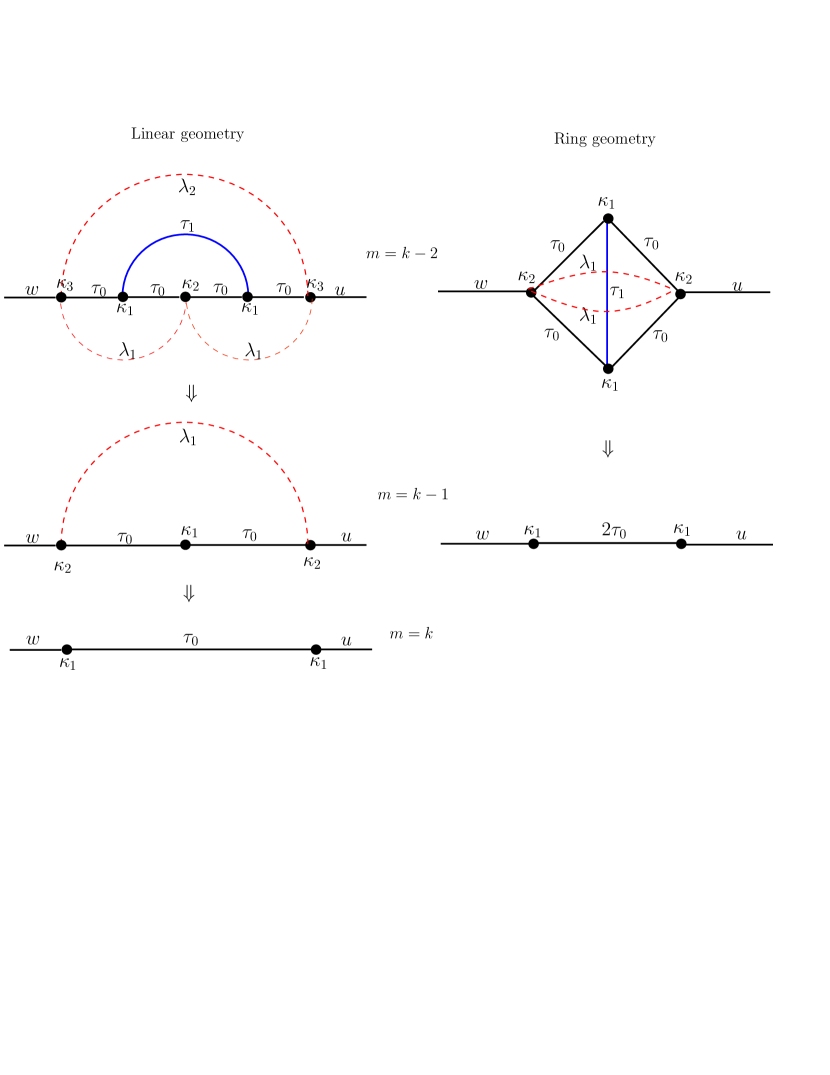
Figure 10: (Color online) The last steps in the RG for the linear (left) and the ring (right) geometries. In both cases one is left with only two sites connected to the external leads. Note for clarity we have dropped the superscripts that denote the RG number on all variables.

Appendix B Transmission from Small Renormalized Lattices

Equations(20 – 24) can be used to construct the $m=k-2$ state shown at the top of Fig. 10. The subsequent RG steps require use of these equations with care.

B.1 Linear geometry

For the linear geometry (left side of Fig. 10), for the $m=k-1$ RG step we proceed as follows. Using the RHS of Eq. (20) with $i=2$ we calculate

$$\tilde{\kappa}_{2}^{(k-1)}=\kappa_{1}^{(k-1)}+\kappa_{k+1}-\kappa_{k}-2(\lambda_{1}^{(k-1)}-\lambda_{k})$$ (61)

and then substitute $\kappa_{2}^{(k-1)}$ by $\tilde{\kappa}_{2}^{(k-1)}$ in the RHS of Eq. (21) to get

$$\kappa_{2}^{(k-1)}=\kappa_{k+1}+\lambda_{k}-\lambda_{1}^{(k-1)}+\frac{1}{2}[\kappa_{1}^{(k-1)}-\kappa_{k}].$$ (62)

This completes the $m=k-1$ RG step. Now for $m=k$, we proceed in a similar way. Using the RHS of Eq. (22) with $m=k-1$ and $\tau_{k}=0$, we calculate

$$\tilde{\kappa}_{1}^{(k)}=\kappa_{1}^{(k-1)}+\kappa_{k+1}-\kappa_{k}-2(\lambda_{1}^{(k-1)}-\lambda_{k})-\frac{2[\tau_{0}^{(k-1)}]^{2}}{\kappa_{1}^{(k-1)}}$$ (63)

and then with $m=k$, $i=2$, $\lambda_{k+1}=0$ and substituting $\kappa_{1}^{(k)}$ by $\tilde{\kappa}_{1}^{(k)}$ in the RHS of Eq. (20), we calculate

$$\tilde{\kappa}_{2}^{(k)}=\tilde{\kappa}_{1}^{(k)}+\kappa_{k+2}-\kappa_{k+1}-2\lambda_{1}^{(k)}\>.$$ (64)

Substituting $m=k-1$ in Eq. (24) gives $\lambda_{1}^{(k)}=0$. Finally, with $m=k$ and substituting $\kappa_{2}^{(k)}$ by $\tilde{\kappa}_{2}^{(k)}$ in the RHS of Eq. (21), we get

$$\kappa_{1}^{(k)} = \kappa_{k+1}+\lambda_{k}-\lambda_{1}^{(k-1)}-\frac{[\tau_{0}^{(k-1)}]^{2}}{\kappa_{1}^{(k-1)}}+\frac{1}{2}[\kappa_{1}^{(k-1)}-\kappa_{k}]$$ (65)

$$= \kappa_{k+1}+\lambda_{k}+\tau_{0}^{(k)}-2\lambda_{1}^{(k-1)}+\frac{1}{2}[\kappa_{1}^{(k-1)}-\kappa_{k}]\>.$$

After performing $k$ RG steps, we are left with just $1+2^{k-k}=2$ sites with an on-site energy corresponding to $\kappa_{1}^{(k)}$ and an interaction of $\tau_{0}^{(k)}$ between them. One site is connected to the input by $w$ while the other is connected to the output by $u$. In order to decimate these two sites, we have

$${\bf A}=\begin{pmatrix}\xi&0\\ 0&\xi\end{pmatrix};\quad\quad{\bf D}=\begin{pmatrix}\kappa_{1}^{(k)}&\tau_{0}^{(k)}\\ \tau_{0}^{(k)}&\kappa_{1}^{(k)}\end{pmatrix};\quad\quad{\bf B}=\begin{pmatrix}w&0\\ 0&u\end{pmatrix}$$ (66)

$${\bf A^{\prime}}={\bf A}-{\bf B}{\bf D}^{-1}{\bf B}^{\rm T}=\begin{pmatrix}\xi-\kappa_{1}^{(k)}\beta/\gamma&\beta\tau_{0}^{(k)}\\ \beta\tau_{0}^{(k)}&\xi-\kappa_{1}^{(k)}\beta\gamma\end{pmatrix}$$ (67)

where $\beta=wu/([\kappa_{1}^{(k)}]^{2}-[\tau_{0}^{(k)}]^{2})$ and $\gamma=u/w$. Thus after decimating all $N=1+2^{k}$ sites, we have

$$\begin{pmatrix}\xi-\kappa_{1}^{(k)}\beta/\gamma&\beta\tau_{0}^{(k)}\\ \beta\tau_{0}^{(k)}&\xi-\kappa_{1}^{(k)}\beta\gamma\end{pmatrix}\begin{pmatrix}1+r\\ t\end{pmatrix}=\begin{pmatrix}2i\Im(\xi)\\ 0\end{pmatrix}.$$ (68)

From the above matrix equation by taking the inverse of the $2\times 2$ matrix,

$$\begin{pmatrix}1+r\\ t\end{pmatrix}=\frac{2i\Im(\xi)}{(\xi-\kappa_{1}^{(k)}\beta/\gamma)(\xi-\kappa_{1}^{(k)}\beta\gamma)-\beta^{2}[\tau_{0}^{(k)}]^{2}}\begin{pmatrix}\xi-\kappa_{1}^{(k)}\beta\gamma\\ -\beta\tau_{0}^{(k)}\end{pmatrix}.$$ (69)

Thus we have found the transmission $T=|t|^{2}$.

Now using Eq. (57) we can calculate the wavefunctions associated with the various sites. For simplicity we take $w=u$. To find the wavefunction associated with the highest level sites ($i=k+1$), we start with the $m=k$ RG step given in Fig. 10. Here, for Eq. (57), $\bm{\psi}=0$, $\mathbf{w_{d}}=\begin{pmatrix}w\\ 0\\ \end{pmatrix}$, $\mathbf{u_{d}}=\begin{pmatrix}0\\ w\\ \end{pmatrix}$ whereas the ${\bf D}$ and ${\bf B}$ matrices are given by Eq. (7). Making these substitutions, we get

$$\bm{\psi}_{k+1}=\frac{-w}{[\kappa_{1}^{(k)}]^{2}-[\tau_{0}^{(k)}]^{2}}\begin{pmatrix}(1+r)\kappa_{1}^{(k)}-t\tau_{0}^{(k)}\\ t\kappa_{1}^{(k)}-(1+r)\tau_{0}^{(k)}\\ \end{pmatrix}.$$ (70)

Next we can find the wavefunction associated with the immediate lower level site ($i=k$). Here, for Eq. (57), $\bm{\psi}=\bm{\psi}_{k+1}$, $\mathbf{w_{d}}=0=\mathbf{u_{d}}$, ${\bf D}=\kappa_{1}^{(k-1)}$ and ${\bf B}=\tau_{0}^{(k-1)}\begin{pmatrix}1\\ 1\\ \end{pmatrix}$. Making these substitutions, we get

$$\bm{\psi}_{k}=\frac{\tau_{0}^{(k-1)}w(1+r+t)}{\kappa_{1}^{(k-1)}[\kappa_{1}^{(k)}+\tau_{0}^{(k)}]}\>.$$ (71)

We can continue in this manner, in principle, to find the wavefunction of all the levels below. However the calculations get very tedious and the expressions very complicated below $i=k$ and therefore are not given explicitly.

B.2 Ring geometry

Next consider the ring geometry (right side of Fig. 10). We perform $k-1$ RG steps to be left with $2^{k-(k-1)}=2$ sites. Site 1 is the nearest neighbor of site 0 and site 2. This makes the interaction between the two sites to be $2\tau_{0}^{(k-1)}$. This adds a factor of $2\lambda_{1}^{(k-1)}$ to the on-site energy of site 0. Thus the on-site energy of the even site 0 corresponds to $(\kappa_{k-1}-2l_{k-1})+2l_{k-1}=\kappa_{k-1}$. The decimation of these two sites is similar to the case of the linear geometry, except that we need to replace $\kappa_{1}^{(k)}$ by $\kappa_{1}^{(k-1)}$ and $\tau_{0}^{(k)}$ by $2\tau_{0}^{(k-1)}$. So $\beta=wu/([\kappa_{1}^{(k-1)}]^{2}-4[\tau_{0}^{(k-1)}]^{2})$ and

$$\begin{pmatrix}1+r\\ t\end{pmatrix}=\frac{2i\Im(\xi)}{(\xi-\kappa_{1}^{(k-1)}\beta/\gamma)(\xi-\kappa_{1}^{(k-1)}\beta\gamma)-4\beta^{2}[\tau_{0}^{(k-1)}]^{2}}\begin{pmatrix}\xi-\kappa_{1}^{(k-1)}\beta\gamma\\ -2\beta\tau_{0}^{(k-1)}\end{pmatrix}.$$ (72)

This completes the RG, giving the transmission $T=|t|^{2}$.

To find the wave functions here, we start at the $m=k-1$ RG step and proceed as we did in the case of the linear geometry. We find that

$$\bm{\psi}_{k} = \frac{-w}{[\kappa_{1}^{(k-1)}]^{2}-4[\tau_{0}^{(k-1)}]^{2}}\>\begin{pmatrix}(1+r)\kappa_{1}^{(k-1)}-2t\tau_{0}^{(k-1)}\\ t\kappa_{1}^{(k-1)}-2(1+r)\tau_{0}^{(k-1)}\\ \end{pmatrix}$$ (73)

and

$$\bm{\psi}_{k-1} = \frac{\tau_{0}^{(k-2)}w(1+r+t)}{[\kappa_{1}^{(k-2)}+\tau_{1}^{(k-2)}][\kappa_{1}^{(k-1)}+2\tau_{0}^{(k-1)}]}\>\begin{pmatrix}1\\ 1\\ \end{pmatrix}.$$ (74)

Notice that the two $i=k-1$ sites are symmetric. Therefore the wavefunctions obtained above for the two sites are identical, as expected. Again the wavefunction expressions for the lower $i$ sites become complicated upon further iteration of this methodology.

References

- (1) V. Pouthier and C. Girardet, Surface Science, 511, 203 (2002).
- (2) P. W. Anderson, Phys. Rev. 109, 1492 (1958).
- (3) Ad Lagendijk, B. van Tiggelen, and D. S. Wiersma, Phys. Today 62, 24 (2009).
- (4) C. Monthus and T. Garel, J. Stat. Mechanics: Theory Exp. P12017 2009.
- (5) C. Monthus and T. Garel, Phys. Rev. B 80, 024203 [11 pages] (2009).
- (6) S. Çali̇şkan, M. A. Novotny, and J. I. Cerdá, J. Appl. Phys. 102, 013707 [7 pages] (2007).
- (7) M. F. Islam and H. Nakanishi, Phys. Rev. E 77, 061109 [9 pages] (2008).
- (8) X.-l. Liu, H. Xu, S.-s. Ma, C.-s. Deng, M.-j. Li, Physica B: Condensed Matter 392, 107 (2007).
- (9) P. M. Ostrovsky, I. V. Gornyi, and A. D. Mirlin, Phys. Rev. B 74, 235443 [20 pages] (2006).
- (10) S. Datta, Electronic Transport in Mesoscopic Systems (Cambridge University Press, Cambridge, U.K., 1997).
- (11) R. F. S. Andrade and H. J. Schellnhuber, Phys. Rev. B 44, 13213 (1991).
- (12) S. Datta, Superlattices and Microstructures 28, 253 (2000).
- (13) Y.-J. Ko, M. Shin, J. S. Ha, and K. W. Park, ETRI Journal 22, 19 (2000).
- (14) V. Pouthier and C. Girardet, Phys. Rev. B 66 115322 [13 pages] (2002).
- (15) D. A. Ryndyk, R. Gutierrez, B. Song, and G. Cuniberti, in Energy Transfer Dynamics in Biomaterial Systems, Springer Series on Chemical Physics, vol. 93, edited by I. Burghard, V. May, D.A. Micha, and E.R. Bittner, (Springer Verlag, Berlin, 2009), p. 213.
- (16) D. Daboul, I. Chang, and A. Aharony, Eur. Phys. J. B 16, 303 (2000).
- (17) L. Solomon and M. A. Novotny, Am. J. Phys. (submitted).
- (18) E. Cuansing, J.-S. Wang, Euro. Phys. J. B — Cond. Matt. and Complex Systems 69, 505 (2009).
- (19) H. Aoki, J. Phys. C: Solid State Phys. 13, 3369 (1980).
- (20) J. R. Banavar and M. Cieplak, Phys. Rev. B 28, 3813 (1983).
- (21) Q. Niu and F. Nori, Phys. Rev. Lett. 57, 2057 (1986).
- (22) D. Mamaluy, M. Sabathil, P. Vogl, J. App. Phys. 93, 4628 (2003).
- Boettcher et al. (2008) S. Boettcher, B. Gonçalves, and H. Guclu, J. Phys. A: Math. Theor. 41, 252001 [7 pages] (2008),
- (24) D. J. Watts, Six Degrees: The Science of a Connected Age, (W. W. Norton & Company, New York, 2004).
- (25) M. A. Novotny and S. M. Wheeler, Braz. J. Phys, 34 395 (2004).
- (26) M. A. Novotny, X. Zhang, J. Yancey, T. Dubreus, M. L. Cook, S. G. Gill, I. T. Norwood, A. M. Novotny, and G. Korniss, J. Appl. Phys. 97, p. 10B309 (2005).
- (27) X. Zhang and M. A. Novotny, Braz. J. Phys. 36, 664 (2006).
- (28) J. A. Yancey, M. A. Novotny, and S. R. Gwaltney, Inter. J. Mod. Phys. C 20, 1345 (2009).
- (29) Y. Gefen, B. B. Mandelbrot, and A. Aharony, Phys. Rev. Lett. 45 855 (1980).
- (30) J. Le Guillou and J. Zinn-Justin, J. Phys. France 48 19 (1987).
- (31) M. A. Novotny, Phys. Rev. B 46, 2939 (1992).
- (32) M. A. Novotny, Phys. Rev. Lett. 70, 109 (1993).
- (33) W. A. Lopes and H. M. Jaeger, Nature 414, 735 (2001).
- (34) A. Böker, et al., Nature Materials 3, 302 (2004).
- (35) Y. Lin, A. Böker, J. He, K. Sill, H. Xiang, C. Abetz, X. Li, J. Wang, T. Emrick, S. Long, Q. Wang, A. Balazs, and T. P. Russell, Nature 434, 55 (2005).
- (36) S. Ravindran and C. S. Ozkan, Nanotechnology 16, 1130 (2005).
- (37) Y. Chen, C. Zhu, X. Shi, M. Cao, and H. Jin, Nanotechnology 19, 205603 [5 pages] (2008).
- Abramowitz and Stegun (1964) M. Abramowitz and I. A. Stegun, Handbook of Mathematical Functions with Formulas, Graphs, and Mathematical Tables (Dover, New York, 1964).
- Otwinowski and Boettcher (2009) J. Otwinowski and S. Boettcher, J. Stat. Mechanics: Theory Exp. 2009, P07010 [21 pages] (2009),
- Boettcher and Goncalves (2008) S. Boettcher and B. Goncalves, Europhysics Letters 84, 30002 [6 pages] (2008),