Electrostatic models of electron-driven proton transfer
across a lipid membrane

Abstract

We present two models for electron-driven uphill proton transport across lipid membranes, with the electron energy converted to the proton gradient via the electrostatic interaction. In the first model, associated with the cytochrome c oxidase complex in the inner mitochondria membranes, the electrostatic coupling to the site occupied by an electron lowers the energy level of the proton-binding site, making the proton transfer possible. In the second model, roughly describing the redox loop in a nitrate respiration of E. coli bacteria, an electron displaces a proton from the negative side of the membrane to a shuttle, which subsequently diffuses across the membrane and unloads the proton to its positive side. We show that both models can be described by the same approach, which can be significantly simplified if the system is separated into several clusters, with strong Coulomb interaction inside each cluster and weak transfer couplings between them. We derive and solve the equations of motion for the electron and proton creation/annihilation operators, taking into account the appropriate Coulomb terms, tunnel couplings, and the interaction with the environment. For the second model, these equations of motion are solved jointly with a Langevin-type equation for the shuttle position. We obtain expressions for the electron and proton currents and determine their dependence on the electron and proton voltage build-ups, on-site charging energies, reorganization energies, temperature, and other system parameters. We show that the quantum yield in our models can be up to 100% and the power-conversion efficiency can reach 35%.

I Introduction

Every living organism obtains the energy needed for its survival from the outside world. This energy can be in the form of sunlight or food; but in both cases it is unstable and cannot be utilized directly, so several energy-conversion steps are necessary. One of the most widely used intermediate forms for energy storage is the electrochemical proton gradient across lipid membranes, such as the inner mitochondrial membranes or plasma membranes in bacteria. To achieve and maintain this proton gradient, nature employs several different types of electron- or light-driven systems, where the energy of high-energetic electrons or absorbed photons is used for the energetically-uphill proton transfer from the negative ($N$) to the positive ($P$) sides of the membrane.

Here we discuss two mechanisms of energy conversion from the highly unstable electronic form of energy to the proton gradient, namely, proton pumps and redox loops Alberts02 ; Nicholls02 . Both mechanisms rely on the electrostatic interaction between electrons and protons, although the specific details of the proton pumps and the redox loops look very different. For example, in a proton pump, such as cytochrome c oxidase, electrons move mainly along the membrane, whereas protons move across the membrane, which results in an accumulation of the positive charge on the $P$-side and in the generation of a proton-motive force (PMF) WV07 ; BelPNAS07 ; Kim07 ; JCPCCO . In the redox-loop mechanism of PMF generation, taking place in the nitrate respiratory chain of E. coli bacterium, the neutral shuttle, carrying both protons and electrons, crosses the membrane. Here, the charge accumulation occurs when electrons cross the membrane, just before embarking on the shuttle, and right after unloading from the shuttle Mitch76 ; Jormakka02 ; Bertero03 ; Gennis05 ; PRERedoxLoop ; JCPPhoto . It should be noted that the proton pump operating in the cytochrome c oxidase has no essential mechanically-moving parts, whereas the redox-loop mechanism is impossible without the molecular shuttle diffusing between the negative and the positive sides of the lipid membrane.

In general, the treatment of the electron and proton transfer events is extremely difficult because the total number of the occupation states increases exponentially with the number of the electron- and proton-binding sites, when all of them are electrostatically coupled. In the present work, however, we show that both above-mentioned mechanisms of the transmembrane proton translocation can be described with a similar mathematical model, taking into account the Coulomb interaction between one electron- and one proton-binding sites only, and neglecting electrostatic couplings to other sites. It is necessary to have at least three redox sites and three proton-binding sites in order to obtain a proton pumping effect and suppress a reverse flow of protons from the $P$-side to the $N$-side of the membrane. In the absence of strong Coulomb interaction between all sites, there is no need to introduce a complete set of electron and proton occupation states (as was done in our previous works, Refs. JCPCCO ; PRERedoxLoop ; JCPPhoto ; PREForster ), which grows exponentially with the number of sites. Instead, we now divide the whole system into clusters of strongly coupled sites. These clusters are described by their own set of occupation states, and the total number of the states in the system is equal to the sum (not the product!) of the states in the clusters. The clusters are weakly coupled by electron tunneling terms and by proton transfer amplitudes, so that transitions between the clusters can be considered within perturbation theory. While in this work we present quite simple models, similar approaches can be applied to much more complicated biological systems, such as Photosystem II and the whole respiratory chain in the inner mitochondrial membrane Nicholls02 .

The quantum yield for the two models analyzed in this paper can be about 1. Why such a high quantum yield? This can be explained from the fact that, in order to be transferred through the system, an electron needs to loose its energy. This cannot be done via the environment because the reorganization energy is not large enough. Consequently, electron transport occurs with the assistance of protons gaining this energy and being transferred to the positive side of the membrane. Thus, the transfer of a single electron is accompanied by the transfer of a single proton and the corresponding currents are equal, which results in an almost perfect quantum yield.

II Model

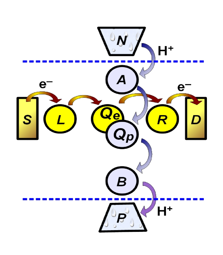
Figure 1: (Color online) Schematic diagram of the static proton pump. The electron transport chain starts at the source ($S$) lead. Thereafter, high-energy electrons, ${\rm e}^{-}$, tunnel energetically-downhill (through the yellow path) to the sites $L,\;Q_{e},\;R$ and, finally, to the drain $D$. Low-energy protons, ${\rm H}^{+}$, move energetically-uphill (in blue) from the negative ($N$) side of the membrane to the sites $A,\;Q_{p},\;B$ and, eventually, reach the positive ($P$) side of the membrane.

We consider a physical model describing an electron-coupled translocation of protons from the negative ($N$) to the positive ($P$) side of a membrane. The model consists of an interaction site, $Q=\{Q_{e},\,Q_{p}\}$, containing a single electron level with energy $\varepsilon_{Q}$ and a single proton energy level characterized by the energy $E_{Q}$. We also introduce two electron sites, $L$ and $R$, coupled to the electron site $Q_{e}$, and two proton sites, $A$ and $B$, coupled to the proton site $Q_{p}$ (Fig. 1). The electron site $L$ is coupled to the electron source $S$, and the site $R$ is connected to the electron drain $D$. The proton site $A$ is coupled to the proton reservoir $N$ (the negative side of the membrane), and the site $B$ is coupled to the positive side of the membrane (proton reservoir $P$).

II.1 Hamiltonian

The Coulomb interaction between an electron and a proton, both located on the central site $Q$, is described by the energy $u_{0}$, so that the Hamiltonian of the site $Q$ has the form

$$H_{Q}=\varepsilon_{Q}n_{Q}+E_{Q}N_{Q}-u_{0}n_{Q}N_{Q},$$ (1)

where $n_{Q}=a_{Q}^{\dagger}a_{Q}$ is the electron population of the site Q, and $N_{Q}=b_{Q}^{\dagger}b_{Q}$ is the proton population of this site. Electrons are described by the Fermi-operators $a_{\sigma}$, and protons are characterized by the Fermi-operators $b_{\alpha}$ with $\sigma=L,Q_{e},R$ and $\alpha=A,Q_{p},C,$ and with the corresponding populations $n_{\sigma}=a_{\sigma}^{\dagger}a_{\sigma},\;N_{\alpha}=b_{\alpha}^{\dagger}b_{\alpha}.$

The contribution of the electron sites $L,R$ and the proton sites $A,B$ to the total Hamiltonian of the system is described by the term

$$H_{0}=\varepsilon_{L}n_{L}+\varepsilon_{R}n_{R}+E_{A}N_{A}+E_{B}N_{B},$$ (2)

where $\varepsilon_{L},\varepsilon_{R}$ are the energy levels of the electron sites $L$ and $R$, and $E_{A},E_{B}$ are the energies of the proton-binding sites $A$ and $B$.

The strongly-interacting electron and proton sites $Q_{e}$ and $Q_{p}$ form a single (interaction) cluster, whereas the sites $L,R$ and $A,B$ separately form other four (peripheral) clusters. The cluster $Q$ can be characterized by the vacuum (empty) state and by three additional occupation states, or, equivalently, by the average electron and proton populations, $\langle n_{Q}\rangle$ and $\langle N_{Q}\rangle$, complemented by the correlation function, $K=\langle n_{Q}N_{Q}\rangle.$ The other electron and proton clusters are described by the corresponding average occupations, $\langle n_{L}\rangle,\;\langle n_{R}\rangle$ and $\langle N_{A}\rangle,\;\langle N_{B}\rangle$. For six electron and proton-binding sites we should have $2^{6}=64$ occupation states. However, with the cluster approach, the system can be completely described by only seven functions: $\langle n_{Q}\rangle,\langle N_{Q}\rangle,K$ (for the interaction cluster), and $\langle n_{L}\rangle,\langle n_{R}\rangle,\langle N_{A}\rangle,\langle N_{B}\rangle$ (for the peripheral clusters). Previously, we applied a similar approach to analyze quantum transport problems in nanomechanical systems RobertPRB .

II.1.1 Electron and proton transitions

The electron tunneling Hamiltonian between the site $Q$ and the sites $L$ and $R$ is given by

$$H_{e}=-\Delta_{L}\,a_{L}^{\dagger}\,a_{Q}-\Delta_{R}\,a_{R}^{\dagger}\,a_{Q}+{\rm H.c.},$$ (3)

whereas the $A$-$Q$ and $B$-$Q$ proton transitions are described by the term

$$H_{p}=-\Delta_{A}\,b_{A}^{\dagger}\,b_{Q}-\Delta_{B}\,b_{B}^{\dagger}\,b_{Q}+{\rm H.c.}.$$ (4)

Here $\Delta_{L},\Delta_{R}$ are the electron tunneling coefficients, and $\Delta_{A},\Delta_{B}$ are the proton transfer amplitudes. In the case of a movable interaction site, e.g., when the electron and proton sites $Q$ are located on the shuttle (quinone/quinol), the amplitudes $\Delta_{L},\Delta_{R}$ and $\Delta_{A},\Delta_{B}$ depend on the position $x$ of the shuttle.

The $S$-lead serves as a source of electrons, and the $D$-lead works as an electron drain. The coupling to these leads is characterized by the Hamiltonian

$$H_{LR}=-\sum_{k}t_{kS}\,c_{kS}^{\dagger}\,a_{L}-\sum_{k}t_{kD}\,c_{kD}^{\dagger}\,a_{R}+{\rm H.c.}$$ (5)

The proton transitions between the $N$-side of the membrane and the site $A$ and between the $P$-side of the membrane and the site $B$ are described by the Hamiltonian

$$H_{AB}=-\sum_{q}T_{qN}\,d_{qN}^{\dagger}\,b_{A}-\sum_{q}T_{qP}\,d_{qP}^{\dagger}\,b_{C}+{\rm H.c.}$$ (6)

Here $c_{kS},c_{kD}$ are Fermi operators of the electron reservoirs $S$ and $D$, and $d_{qN},d_{qP}$ are the Fermi operators of protons in the reservoirs $N$ and $P$. The electron reservoirs $S$ and $D$ have the Hamiltonian

$$H_{SD}=\sum_{k}(\varepsilon_{kS}\,c_{kS}^{\dagger}\,c_{kS}+\varepsilon_{kD}\,c_{kD}^{\dagger}\,c_{kD}),$$ (7)

and are characterized by the Fermi distributions $f_{S}(\varepsilon_{kS}),f_{D}(\varepsilon_{kD})$ with the corresponding electrochemical potentials $\mu_{S}$ and $\mu_{D}$. For the proton reservoirs $N$ and $P$ we have the Hamiltonian

$$H_{NP}=\sum_{q}(E_{qN}\,d_{qN}^{\dagger}\,d_{qN}+E_{qP}\,d_{qP}^{\dagger}\,d_{qP}),$$ (8)

with the Fermi distributions $F_{N}(E_{qN})$ and $F_{P}(E_{qP})$ and the proton electrochemical potentials $\mu_{N}$ and $\mu_{P}$.

II.1.2 Environment

The interaction of the electron-proton system with the protein environment, which is described as a sum of independent oscillators Krish01 , is characterized by the Hamiltonian

$$H_{\rm env}=\sum_{j}\frac{p_{j}^{2}}{2m_{j}}+\sum_{j}\frac{m_{j}\omega_{j}^{2}}{2}\left(x_{j}-\sum_{\sigma}x_{j\sigma}n_{\sigma}-x_{jS}\sum_{k}c_{kS}^{\dagger}c_{kS}-x_{jD}\sum_{k}c_{kD}^{\dagger}c_{kD}-\right.$$

$$\left.\sum_{\alpha}X_{j\alpha}N_{\alpha}-X_{jN}\sum_{q}d_{qN}^{\dagger}d_{qN}-X_{jP}\sum_{q}d_{qP}^{\dagger}d_{qP}\right)^{2},$$ (9)

where $n_{\sigma}=a_{\sigma}^{\dagger}a_{\sigma}$ is the population of the electron site $\sigma$ ($\sigma=L,Q,R$), $N_{\alpha}=b_{\alpha}^{\dagger}b_{\alpha}$ is the population of the proton site $\alpha$ ($\alpha=A,Q,B$). The constants $x_{j\sigma},x_{jS},x_{jD}$ determine the electron coupling to the environment, and the parameters $X_{j\alpha},X_{jN},X_{jP}$ describe the proton-environment interaction.

With the unitary transformation,

$${\cal U}=\exp\bigg{[}-i\sum_{j}p_{j}\bigg{(}\sum_{\sigma}x_{j\sigma}n_{\sigma}+x_{jS}\sum_{k}c_{kS}^{\dagger}c_{kS}+x_{jD}\sum_{k}c_{kD}^{\dagger}c_{kD}+$$

$$\sum_{\alpha}X_{j\alpha}N_{\alpha}+X_{jN}\sum_{q}d_{qN}^{\dagger}d_{qN}+X_{jP}\sum_{q}d_{qP}^{\dagger}d_{qP}\bigg{)}\bigg{]},$$ (10)

the environment Hamiltonian can be rewritten as

$$H_{\rm env}=\sum_{j}\left(\frac{p_{j}^{2}}{2m_{j}}+\frac{m_{j}\omega_{j}^{2}x_{j}^{2}}{2}\right),$$ (11)

whereas the Hamiltonians $H_{e}$ and $H_{p}$ acquire the stochastic phase factors:

$$H_{e}=-\Delta_{L}\,e^{i\xi_{L}}\,a_{L}^{\dagger}\,a_{Q}-\Delta_{R}\,e^{i\xi_{R}}\,a_{R}^{\dagger}\,a_{Q}+{\rm H.c.},$$ (12)

and

$$H_{p}=-\Delta_{A}\,e^{i\xi_{A}}\,b_{A}^{\dagger}\,b_{Q}-\Delta_{B}\,e^{i\xi_{B}}\,b_{B}^{\dagger}\,b_{Q}+{\rm H.c.}$$ (13)

with the phases

$$\xi_{L}=\sum_{j}p_{j}(x_{jL}-x_{jQ}),$$

$$\xi_{R}=\sum_{j}p_{j}(x_{jR}-x_{jQ}),$$

and

$$\xi_{A}=\sum_{j}p_{j}(X_{jA}-X_{jQ}),$$

$$\xi_{B}=\sum_{j}p_{j}(X_{jB}-X_{jQ}).$$

For simplicity, we assume that there are no phase shifts for the electron transitions between the electron source $S$ and the site $L$, and the electron drain $D$ and the site $R$, so that $x_{jS}=x_{jL},$ and $x_{jD}=x_{jR}$, with the same assumption for the $N$-$A$ and $P$-$B$ proton transitions, $X_{jN}=X_{jA}$ and $X_{jP}=X_{jB}.$

II.2 Rate equations

The time evolution of the electron operators $n_{\sigma}$ is determined by the Heisenberg equations:

$$\dot{n}_{L}=i\Delta_{L}\,e^{i\xi_{L}}\,a_{L}^{\dagger}\,a_{Q}-i\sum_{k}t_{kS}\,c_{kS}^{\dagger}\,a_{L}+{\rm H.c.},$$

$$\dot{n}_{R}=i\Delta_{R}\,e^{i\xi_{R}}\,a_{R}^{\dagger}\,a_{Q}-i\sum_{k}t_{kD}\,c_{kD}^{\dagger}\,a_{R}+{\rm H.c.},$$ (14)

and

$$\dot{n}_{Q}=-i\Delta_{L}\,e^{i\xi_{L}}\,a_{L}^{\dagger}\,a_{Q}-i\Delta_{R}\,e^{i\xi_{R}}\,a_{R}^{\dagger}\,a_{Q}+{\rm H.c.}$$ (15)

For the proton populations $N_{\alpha}$, we derive the similar set of Heisenberg equations,

$$\dot{N}_{A}=i\Delta_{A}\,e^{i\xi_{A}}\,b_{A}^{\dagger}\,b_{Q}-i\sum_{q}T_{qN}\,d_{qN}^{\dagger}\,b_{A}+{\rm H.c.},$$

$$\dot{N}_{B}=i\Delta_{B}\,e^{i\xi_{B}}\,b_{B}^{\dagger}\,b_{Q}-i\sum_{q}T_{qP}\,d_{qP}^{\dagger}\,b_{B}+{\rm H.c.}$$ (16)

This set should be complemented by the equation for the proton population of the interaction site,

$$\dot{N}_{Q}=-i\Delta_{A}\,e^{i\xi_{A}}\,b_{A}^{\dagger}\,b_{Q}-i\Delta_{B}\,e^{i\xi_{B}}\,b_{B}^{\dagger}\,b_{Q}+{\rm H.c.},$$ (17)

as well as by the equations for the operators of electron and proton reservoirs,

$$i\,\dot{c}_{kS} = \varepsilon_{kS}\,c_{kS}-t_{kS}\,a_{L},$$

$$i\,\dot{c}_{kD} = \varepsilon_{kD}\,c_{kD}-t_{kD}\,a_{R},$$ (18)

$$i\,\dot{d}_{qN} = E_{qN}\,d_{qN}-T_{qN}\,b_{A},$$

$$i\,\dot{d}_{qP} = E_{qP}\,d_{qP}-T_{qP}\,b_{B}.$$ (19)

II.2.1 Contribution of reservoirs to the rate equations

It follows from Eq. (18) that the electron operator $c_{kS}$ can be represented as

$$c_{kS}=c_{kS}^{(0)}-t_{kS}\int dt_{1}\langle-i[c_{kS}^{(0)}(t),c_{kS}^{(0){\dagger}}(t_{1})]_{+}\rangle\,a_{L}(t_{1})\,\theta(t-t_{1}),$$ (20)

where $c_{kS}^{(0)}(t)$ is the free variable of the $S$-lead, and $\theta(t-t_{1})$ is the Heaviside step function. Similar expressions take place for the electron operator $c_{kD}(t)$ and for operators $d_{qN},d_{qP}$ of the proton reservoirs. For the weak coupling between the reservoir $S$ and the electron site $L$ we obtain

$$\langle a_{L}^{\dagger}(t)c_{kS}^{(0)}(t)\rangle=-it_{kS}\int dt_{1}\langle c_{kS}^{(0){\dagger}}(t_{1})c_{kS}^{(0)}(t)\rangle\,\langle[a_{L}(t_{1}),a_{L}^{\dagger}(t)]_{+}\rangle\,\theta(t-t_{1}).$$ (21)

Thus, contribution of the $S$-lead to the evolution of the average electron population $\langle n_{L}\rangle$ (see Eq. (14)) is determined by the expression

$$i\,\sum_{k}t_{kS}^{*}\langle a_{L}^{\dagger}(t)c_{kS}(t)\rangle=-\sum_{k}|t_{kS}|^{2}\int dt_{1}\{\langle c_{kS}^{(0)}(t)c_{kS}^{(0){\dagger}}(t_{1})\rangle\,\langle a_{L}^{\dagger}(t)a_{L}(t_{1})\rangle-$$

$$\langle c_{kS}^{(0){\dagger}}(t_{1})c_{kS}^{(0)}(t)\rangle\,\langle a_{L}(t_{1})a_{L}^{\dagger}(t)\rangle\}.$$ (22)

The correlator $\langle c_{kS}^{(0){\dagger}}(t_{1})c_{kS}^{(0)}(t)\rangle$ is proportional to the Fermi distribution function, $f_{S}(\varepsilon_{kS})$ of electrons in the reservoir $S$,

$$\langle c_{kS}^{(0){\dagger}}(t_{1})c_{kS}^{(0)}(t)\rangle=f_{S}(\varepsilon_{kS})\,e^{-i\varepsilon_{kS}(t-t_{1})},$$ (23)

where the Fermi function,

$$f_{S}(\varepsilon)=\left[\exp\left(\frac{\varepsilon-\mu_{S}}{T}\right)+1\right]^{-1},$$

is characterized by the electrochemical potential $\mu_{S}$ and temperature $T$. We assume that the site $L$ is weakly-coupled to the reservoir $S$ and to the site $Q$, thus, we can use free-evolving operators,

$$a_{L}(t)=e^{-i\varepsilon_{L}(t-t_{1})}\,a_{L}(t_{1}),$$

to calculate the corresponding correlation functions in Eq. (22), e.g.,

$$\langle a_{L}^{\dagger}(t)\,a_{L}(t_{1})\rangle=\langle n_{L}(t)\rangle\,e^{i\varepsilon_{L}(t-t_{1})}.$$

Introducing the energy-independent rate constant,

$$\gamma_{S}=2\pi\sum_{k}|t_{kS}|^{2}\,\delta(\varepsilon_{L}-\varepsilon_{kS}),$$ (24)

we calculate the contribution of the $S$-lead to the time evolution of the population $\langle n_{L}\rangle$,

$$i\,\sum_{k}t_{kS}^{*}\,\langle a_{L}^{\dagger}(t)c_{kS}(t)\rangle+{\rm H.c.}=\gamma_{S}\,[f_{S}(\varepsilon_{L})-\langle n_{L}\rangle].$$ (25)

The same analysis can be applied for a calculation of contributions of the electron lead $D$ and the proton leads $N$ and $P$ to the corresponding populations $\langle n_{R}\rangle$ and $\langle N_{A}\rangle,\langle N_{P}\rangle.$ The proton transfer rates between the sites $A$ and $C$ and the negative and positive sides of the membrane, respectively, are determined by the coefficients $\Gamma_{N}$ and $\Gamma_{P}$ where, e.g.,

$$\Gamma_{N}=2\pi\sum_{q}|T_{qN}|^{2}\,\delta(E_{A}-E_{qN}).$$ (26)

II.2.2 Contribution of site-to-site tunneling to the rate equations

To calculate a contribution of the $L$-$Q$ tunneling to the evolution of the populations $\langle n_{L}\rangle$ and $\langle n_{Q}\rangle$, we start with the amplitude $a_{Q}$, which obeys the equation

$$i\dot{a}_{Q}=\varepsilon_{Q}\,a_{Q}-u_{0}\,N_{Q}\,a_{Q}-\Delta_{L}^{*}\,e^{-i\xi_{L}}\,a_{L}-\Delta_{R}^{*}\,e^{-i\xi_{R}}\,a_{R}.$$ (27)

In the case of weak $L$-$Q$ and $R$-$Q$ tunnel couplings, the formal solution of Eq. (27) can be written in the form

$$a_{Q}(t)=a_{Q}^{(0)}(t)-$$

$$\int dt_{1}\langle-i[a_{Q}^{(0)}(t),a_{Q}^{(0){\dagger}}(t_{1})]_{+}\rangle\,\{\Delta_{L}^{*}\,e^{-i\xi_{L}(t_{1})}\,a_{L}(t_{1})+\Delta_{R}^{*}\,e^{-i\xi_{R}(t_{1})}\,a_{R}(t_{1})\},$$ (28)

where $a_{Q}^{(0)}(t)$ is the free operator of the site $Q$, obeying the equation (27) with the tunneling terms neglected ($\Delta_{L}=0,\Delta_{R}=0)$.

Taking into account the formula,

$$i\Delta_{L}\,\langle e^{i\xi_{L}}\,a_{L}^{\dagger}\,a_{Q}^{(0)}\rangle=$$

$$|\Delta_{L}|^{2}\,\int dt_{1}\langle a_{Q}^{(0){\dagger}}(t_{1})a_{Q}^{(0)}(t)\rangle\,\langle[e^{i\xi_{L}}(t)\,a_{L}^{\dagger}(t),\,e^{-i\xi_{L}(t_{1})}\,a_{L}(t_{1})]_{+}\rangle\,\theta(t-t_{1}),$$ (29)

which is similar to Eq. (21), we obtain

$$i\Delta_{L}\,\langle e^{i\xi_{L}}\,a_{L}^{\dagger}\,a_{Q}\rangle=|\Delta_{L}|^{2}\,\int dt_{1}\{\langle e^{-i\xi_{L}(t_{1})}\,e^{i\xi_{L}(t)}\rangle\langle a_{Q}^{\dagger}(t_{1})\,a_{Q}(t)\rangle\,\langle a_{L}(t_{1})\,a_{L}^{\dagger}(t)\rangle-$$

$$\langle e^{i\xi_{L}(t)}\,e^{-i\xi_{L}(t_{1})}\rangle\,\langle a_{Q}(t)\,a_{Q}^{\dagger}(t_{1})\rangle\,\langle a_{L}^{\dagger}(t)\,a_{L}(t_{1})\rangle\}.$$ (30)

Dropping the label ⁽⁰⁾, we assume that the time evolution of the operators $a_{Q}$ in Eq. (30) is calculated with the free-evolution formula,

$$a_{Q}(t)=e^{-i\varepsilon_{Q}(t-t_{1})}\,a_{Q}(t_{1})-e^{-i\varepsilon_{Q}(t-t_{1})}\,[1-e^{iu_{0}(t-t_{1})}]\,N_{Q}(t_{1})\,a_{Q}(t_{1}).$$ (31)

For the free-evolving proton operator of the interaction site we obtain a similar expression

$$b_{Q}(t)=e^{-iE_{Q}(t-t_{1})}\,b_{Q}(t_{1})-e^{-iE_{Q}(t-t_{1})}\,[1-e^{iu_{0}(t-t_{1})}]\,n_{Q}(t_{1})\,b_{Q}(t_{1}).$$ (32)

The influence of the environment on the electron tunneling between the sites $L$ and $Q$, and between the sites $R$ and $Q$, is determined by the correlators $\langle e^{-i\xi_{L}(t_{1})}\,e^{i\xi_{L}(t)}\rangle$ and $\langle e^{i\xi_{L}(t)}\,e^{-i\xi_{L}(t_{1})}\rangle$, where

$$\langle e^{i\xi_{L}(t)}\,e^{-i\xi_{L}(t_{1})}\rangle=\exp\{-i\lambda_{L}(t-t_{1})\}\,\exp\{-\lambda_{L}T(t-t_{1})^{2}\}.$$ (33)

The reorganization energy, $\lambda_{L}$, is defined as Krish01

$$\lambda_{L}=\sum_{j}\frac{m_{j}\omega_{j}^{2}}{2}(x_{jL}-x_{jQ})^{2}.$$ (34)

The electron reorganization energy $\lambda_{R}$, and the proton reorganization energies $\Lambda_{A}$ and $\Lambda_{B},$ are defined in a similar way. In particular,

$$\Lambda_{A}=\sum_{j}\frac{m_{j}\omega_{j}^{2}}{2}(X_{jA}-X_{jQ})^{2}.$$ (35)

II.2.3 Equations for populations of electron and proton-binding sites

Consequently, we derive the system of rate equations for the average populations of the electron sites,

$$\dot{n}_{L}+\gamma_{S}n_{L}=\gamma_{S}f_{S}(\varepsilon_{L})+\Phi_{L},$$

$$\dot{n}_{R}+\gamma_{D}n_{R}=\gamma_{D}f_{D}(\varepsilon_{R})+\Phi_{R},$$

$$\dot{n}_{Q}=-\Phi_{L}-\Phi_{R},$$ (36)

and for the average populations of the proton-binding sites,

$$\dot{N}_{A}+\Gamma_{N}N_{A}=\Gamma_{N}F_{N}(E_{A})+\Phi_{A},$$

$$\dot{N}_{B}+\Gamma_{P}N_{B}=\Gamma_{P}F_{P}(E_{B})+\Phi_{B},$$

$$\dot{N}_{Q}=-\Phi_{A}-\Phi_{B}.$$ (37)

Here $\Phi_{\sigma}$ ($\sigma=L,R$) and $\Phi_{\alpha}$ ($\alpha=A,B$) are the functions of the average electron and proton populations, respectively. In addition, due to a strong electron-proton Coulomb interaction on the site $Q$, the kinetic terms $\Phi_{\sigma}$ and $\Phi_{\alpha}$ depend on the correlation function,

$$\langle K\rangle=\langle n_{Q}(t)N_{Q}(t)\rangle,$$ (38)

of the electron and proton populations on the site Q,

$$\Phi_{\sigma}=\kappa_{\sigma}(\varepsilon_{\sigma}-\varepsilon_{Q}+\lambda_{\sigma})\langle n_{Q}\rangle\langle 1-n_{\sigma}\rangle-\kappa_{\sigma}(\varepsilon_{\sigma}-\varepsilon_{Q}-\lambda_{\sigma})\langle 1-n_{Q}\rangle\langle n_{\sigma}\rangle+$$

$$\{\kappa_{\sigma}(\varepsilon_{\sigma}-\varepsilon_{Q}+u_{0}+\lambda_{\sigma})-\kappa_{\sigma}(\varepsilon_{\sigma}-\varepsilon_{Q}+\lambda_{\sigma})\}\langle 1-n_{\sigma}\rangle\langle K\rangle-$$

$$\{\kappa_{\sigma}(\varepsilon_{\sigma}-\varepsilon_{Q}+u_{0}-\lambda_{\sigma})-\kappa_{\sigma}(\varepsilon_{\sigma}-\varepsilon_{Q}-\lambda_{\sigma})\}\langle n_{\sigma}\rangle\langle N_{Q}-K\rangle,$$ (39)

where $\kappa_{\sigma}(\varepsilon)$ is the Marcus rate for electron transfer between the site $\sigma$ and the interaction site $Q$,

$$\kappa_{\sigma}(\varepsilon)=|\Delta_{\sigma}|^{2}\sqrt{\frac{\pi}{\lambda_{\sigma}T}}\exp\left(-\frac{\varepsilon^{2}}{4\lambda_{\sigma}T}\right).$$ (40)

The proton term $\Phi_{\alpha}$ is determined by the expression, similar to Eq. (39), as

$$\Phi_{\alpha}=\kappa_{\alpha}(E_{\alpha}-E_{Q}+\Lambda_{\alpha})\langle N_{Q}\rangle\langle 1-N_{\alpha}\rangle-\kappa_{\alpha}(E_{\alpha}-E_{Q}-\Lambda_{\alpha})\langle 1-N_{Q}\rangle\langle N_{\alpha}\rangle+$$

$$\{\kappa_{\alpha}(E_{\alpha}-E_{Q}+u_{0}+\Lambda_{\alpha})-\kappa_{\alpha}(E_{\alpha}-E_{Q}+\Lambda_{\alpha})\}\langle 1-N_{\alpha}\rangle\langle K\rangle-$$

$$\{\kappa_{\alpha}(E_{\alpha}-E_{Q}+u_{0}-\Lambda_{\alpha})-\kappa_{\alpha}(E_{\alpha}-E_{Q}-\Lambda_{\alpha})\}\langle N_{\alpha}\rangle\langle n_{Q}-K\rangle,$$ (41)

where $\kappa_{\alpha}(E)$ is the proton Marcus rate for the transitions between the site $\alpha$ and the proton-binding site $Q$,

$$\kappa_{\alpha}(E)=|\Delta_{\alpha}|^{2}\sqrt{\frac{\pi}{\Lambda_{\alpha}T}}\exp\left(-\frac{E^{2}}{4\Lambda_{\alpha}T}\right).$$ (42)

II.2.4 Equation for the electron-proton correlation function

For the correlator, $\langle K\rangle$, of the electron ($n_{Q}$) and proton ($N_{Q}$) populations of the interaction site, we derive the following equation

$$\langle\dot{K}\rangle={\cal F}_{L}+{\cal F}_{R}+{\cal F}_{A}+{\cal F}_{B},$$ (43)

where

$${\cal F}_{\sigma}=\kappa_{\sigma}(\varepsilon_{\sigma}-\varepsilon_{Q}+u_{0}-\lambda_{\sigma})\langle n_{\sigma}\rangle\langle N_{Q}-K\rangle-$$

$$\kappa_{\sigma}(\varepsilon_{\sigma}-\varepsilon_{Q}+u_{0}+\lambda_{\sigma})\langle 1-n_{\sigma}\rangle\langle K\rangle,$$

$${\cal F}_{\alpha}=\kappa_{\alpha}(E_{\alpha}-E_{Q}+u_{0}-\Lambda_{\alpha})\langle N_{\alpha}\rangle\langle n_{Q}-K\rangle-$$

$$\kappa_{\alpha}(E_{\alpha}-E_{Q}+u_{0}+\Lambda_{\alpha})\langle 1-N_{\alpha}\rangle\langle K\rangle.$$ (44)

II.2.5 Electron and proton currents

Electron currents $I_{S},I_{D}$ and proton currents $I_{N},I_{P}$ are determined by an increase of the number of particles, electrons or protons, in the corresponding reservoir. In particular, a variation of the electron number in the drain lead gives a current

$$I_{D}=\frac{d}{dt}\sum_{k}\langle c_{kD}^{\dagger}c_{kD}\rangle=\gamma_{D}[\langle n_{R}\rangle-f_{D}(\varepsilon_{R})],$$ (45)

whereas the proton current $I_{P}$ is given by

$$I_{P}=\frac{d}{dt}\sum_{q}\langle d_{qP}^{\dagger}d_{qP}\rangle=\Gamma_{P}[\langle N_{B}\rangle-F_{P}(E_{B})].$$ (46)

Here,

$$\gamma_{D}=2\pi\sum_{k}|t_{kD}|^{2}\delta(\varepsilon_{R}-\varepsilon_{kD}),$$

and

$$\Gamma_{P}=2\pi\sum_{q}|T_{qP}|^{2}\delta(E_{B}-E_{qP})$$

are the electron ($\gamma_{D}$) and proton ($\Gamma_{P}$) transfer rates between the electron site $R$ and the lead $D$, and between the proton-binding site $B$ and the $P$-side of the membrane, respectively. The multiplications of the particle currents introduced above by the electron or proton charges produce the standard electric currents.

It follows from Eqs. (36,37) that, in the steady-state, we have the relations:

$$\langle\dot{n}_{\sigma}\rangle=0\,,\;\langle\dot{N}_{\alpha}\rangle=0\,,$$

so that

$$\Phi_{L}+\Phi_{R}=0\,,$$

$$\Phi_{A}+\Phi_{B}=0\,,$$

and

$$I_{S}=(d/dt)\sum_{k}\langle c_{kS}^{\dagger}c_{kS}\rangle=-I_{D},$$

$$I_{N}=(d/dt)\sum_{q}\langle d_{qN}^{\dagger}d_{qN}\rangle=-I_{P}.$$

II.2.6 Quantum yield of the electron-driven proton pump

The productivity of the proton pump is determined by a quantum yield,

$$QY=\frac{I_{P}}{I_{D}},$$ (47)

and by the power-conversion efficiency $\eta$,

$$\eta=QY\times\frac{\mu_{P}-\mu_{N}}{\mu_{S}-\mu_{D}}.$$ (48)

At the standard conditions, we have

$$\mu_{P}-\mu_{N}=V_{p}+60~{}{\rm meV}=210~{}{\rm meV},$$

and

$$\mu_{S}-\mu_{D}=V_{e}=600~{}{\rm meV},$$

therefore,

$$\eta\simeq 0.35\times QY.$$

If a quantum yield $QY$ is of order one (or 100%), the power-conversion efficiency $\eta$ may be as much as 0.35 (or 35%).

II.3 Langevin equation

For the redox-loop mechanism of a proton translocation through the membrane, the electron and proton sites, labelled by the letter $Q$, are attached to the shuttle: a molecule diffusing between the $N$ and $P$ sides of the membrane (see Fig. 2). This Brownian motion can be described by the one-dimensional overdamped Langevin equation for the coordinate $x$ of the shuttle,

$$\zeta\dot{x}=-\,\frac{dU_{c}(x)}{dx}-\Big{\langle}(n_{Q}-N_{Q})^{2}\Big{\rangle}\,\frac{dU_{s}(x)}{dx}+\xi.$$ (49)

We assume that the shuttle molecule moves along a line connecting the sites $L$ and $A$, located at $x=-x_{0}$, and the sites $R$ and $B$, both having the coordinate $x=x_{0}$. The borders of the membrane, at $x=\pm x_{0},$ are schematically shown in Fig. 2. In Eq. (49), $\zeta$ is the drag coefficient of the shuttle, and $\xi$ is the Gaussian fluctuation force, which is characterized by the zero-mean value, $\langle\xi\rangle=0$, and the correlation function,

$$\langle\xi(t)\xi(t^{\prime})\rangle~{}=~{}2\zeta T\delta(t-t^{\prime})\,,$$

proportional to the temperature $T$ of the environment. The diffusion coefficient $D$ of the shuttle is also proportional to the temperature: $D=T/\zeta.$ The motion of the shuttle is restricted by the membrane walls, which are simulated by the confinement potential $U_{c}(x)$,

$$U_{c}(x)=U_{c0}\left\{1-\left[\exp\left(\frac{x-x_{c}}{l_{c}}\right)+1\right]^{-1}+\left[\exp\left(\frac{x+x_{c}}{l_{c}}\right)+1\right]^{-1}\right\},$$ (50)

having the barrier height $U_{c0}$, the width $2x_{c}\ (x_{c}\geq x_{0})$ and the steepness $l_{c}$.

The potential barrier $U_{s}(x)$,

$$U_{s}(x)=U_{s0}\left\{\left[\exp\left(\frac{x-x_{s}}{l_{s}}\right)+1\right]^{-1}-\left[\exp\left(\frac{x+x_{s}}{l_{s}}\right)+1\right]^{-1}\right\},$$ (51)

does not allow the shuttle with a non-zero charge $q=N_{Q}-n_{Q}$ (in units of $|e|$) to cross the lipid interior of the membrane. This barrier is determined by the height $U_{s0}$, the steepness $l_{s}$, and the width $2x_{s}$.

III Results

We solve the rate equations (36,37) for the electron ($n_{\sigma}$) and proton ($N_{\alpha}$) populations jointly with the equation (43) for the electron-proton correlation function on the site $Q$, $K=\langle n_{Q}N_{Q}\rangle$. Our approach can describe two mechanisms of the redox-linked proton translocation across the membrane: (i) the static interaction site $Q$ and (ii) the situation when the site $Q$ diffuses between the sides of the membrane. The mechanism (i) roughly corresponds to the proton pump operating in cytochrome c oxidase (CcO) WV07 ; BelPNAS07 ; Kim07 ; JCPCCO , whereas the design (ii) can be attributed to the redox loop mechanism, which is responsible for electron and proton transfers in the inner membrane of bacteria Mitch76 ; Jormakka02 ; Bertero03 ; Gennis05 ; PRERedoxLoop ; JCPPhoto .

III.1 Static proton pump

Here, we consider the mechanism (i), where the interaction site $Q$ does not change its position (see Fig. 1). We assume that protons are transferred across the membrane, from the negatively charged side $N$, with an electrochemical potential $\mu_{N}$, to the positively charged side $P$, having an electrochemical potential $\mu_{P}$. All potentials and energies are measured in meV.

III.1.1 Parameters

The difference of electrochemical potentials, $\Delta\mu_{H}=\mu_{P}-\mu_{N},$ is determined by the following expression

$$\Delta\mu_{H}=V_{p}-2.3\,(RT/F)\times\Delta pH,$$ (52)

where $V_{p}$ is the transmembrane voltage, $R$ and $F$ are the gas and Faraday constants, respectively, $T$ is the temperature (in Kelvins, $k_{B}=1$), and the concentration gradient $\Delta pH$ is about $-1$. Alberts02 ; Nicholls02 . The coefficient $2.3\,(RT/F)$ is about 60 meV at room temperature, $T=T_{0}\equiv~{}298~{}$K. It follows from Eq. (52) that the potentials of the $N$ and $P$ sides of the membrane can be written as

$$\mu_{N} = -\mu_{H0}-\Delta V_{p}/2-30\times(\Delta T/T_{0}),$$

$$\mu_{P} = \mu_{H0}+\Delta V_{p}/2+30\times(\Delta T/T_{0}),$$ (53)

where $\Delta V_{p}=V_{p}-V_{0},\;\Delta T=T-T_{0}.$ At the standard conditions, when $T=T_{0}$, $V_{p}=V_{0}=150$ meV, for the electrochemical potential $\mu_{H0}$ we have: $\mu_{H0}=105$ meV. Thus, the total proton gradient across the membrane, $\Delta\mu_{H}$, is about 210 meV. As in the CcO proton pump WV07 ; JCPCCO , we assume that the proton-binding sites $A,Q_{p}$, and $B$ are located approximately on the line connecting the $N$ and $P$ sides of the membrane with the following coordinates: $x_{A}=0.1,\;x_{Q}=0.3,\;x_{B}=0.5.$ The coordinates of the sites are counted from the middle of the membrane in a direction towards the $P$-side and are measured in units of the membrane width $W$ with $W\simeq 4$ nm. Protons are delivered from the $N$-side to the site $A$ by the so-called $D$-pathway crossing about a half of the membrane. We also note that the $B$-site is located next to the $P$-side (see Fig. 1). An influence of the transmembrane voltage $V_{p}$ on the energy levels of the proton sites is described by the formulas

$$E_{A}=E_{A0}+x_{A}\times\Delta V,$$

$$E_{Q}=E_{Q0}+x_{Q}\times\Delta V,$$

$$E_{B}=E_{B0}+x_{B}\times\Delta V.$$ (54)

For the proton energy levels, $E_{A0},E_{Q0}$, and $E_{B0}$, at the voltage $V_{p}=V_{0}$, we assume the following values (in meV): $E_{A0}=-155,E_{Q0}=250$, and $E_{B0}=185,$ unless otherwise specified. This means that at the standard conditions, the proton begins its journey at the $N$-side with the potential $\mu_{N}=-105$ meV and jumps to the $A$-site having a lower energy ($-155$ meV). However, the next proton-binding site $Q_{p}$ has a much higher energy ($\sim 250$ meV), so that the proton transfer cannot occur without a mediation of the electron component. The electron site $Q_{e}$ is electrostatically coupled to the proton-binding site $Q_{p}$ with the Coulomb energy $u_{0}$. Thus, in the presence of an electron on the site $Q_{e}$ the energy of the $Q$-proton decreases to the level $E_{Q0}-u_{0}\simeq-220$ meV, provided that $u_{0}\simeq 470$ meV. Now the proton can move from site $A$ to site $Q$, since $E_{A0}>E_{Q0}-u_{0}$. Depopulation of the electron site $Q$ returns the energy level of the $Q$-proton to its original value $E_{Q0}=250$ meV, which is higher than the energy level of the next-in-line $B$ site, $E_{B0}=185$ meV, and is much higher than the energy level of the $A$-site. We assume that the backward proton transfer (from $Q_{p}$ to $A$ site) is described by the inverted region of the Marcus formula, so that the probability of such transfer is low, compared to the probability of the proton transfer from the site $Q_{p}$ to the site $B$. No additional gate mechanism is necessary here.

For the sake of simplicity, we assume that three electron-binding sites $L,Q_{e},R$ as well as the source and drain leads are positioned on a line, which is parallel to the surface of the membrane (see Fig. 1). Thus, the transmembrane gradient $V_{p}$ has no effect on electron transport from the electron source $S$ to the drain $D$. For the potentials of the electron reservoirs, we choose the following form

$$\mu_{S}=\mu_{e0}+V_{e}/2,$$

$$\mu_{D}=\mu_{e0}-V_{e}/2,$$ (55)

with $\mu_{e0}=-500$ meV and with the electron voltage gradient $V_{e}=600$ meV, unless otherwise indicated. The electron voltage gradient $V_{e}$ roughly corresponds to the drop of the redox potential along the electron transfer chain in the cytochrome c oxidase Alberts02 ; Nicholls02 ; WV07 . We assume that the electron pathway includes the source reservoir ($\mu_{S}=-200$ meV), the site $L$ ($\varepsilon_{L}=-210$ meV), the interaction site $Q_{e}$ ($\varepsilon_{Q}=-250$ meV), the site $R$ ($\varepsilon_{R}=-770$ meV), and the electron drain reservoir having the potential $\mu_{D}=-800$ meV.

We assume that the electron and proton transfer between the active sites, $L$-$Q$, $R$-$Q$ and $A$-$Q$, $B$-$Q$, are quite fast, with amplitudes $\Delta_{L}\simeq\Delta_{R}\simeq 0.3$/ps and $\Delta_{A}\simeq\Delta_{B}\simeq 0.3$/ps, whereas the transitions to and out the electron and proton reservoirs are characterized by much slower rates: $\gamma_{S}\simeq\gamma_{D}\simeq 1.5$/ns, and $\Gamma_{N}\simeq\Gamma_{D}\simeq 0.75$/ns. The responses of the environment to the electron and proton transitions are described by the corresponding reorganization energies: $\lambda_{L}=\lambda_{R}=\lambda_{e}$ and $\Lambda_{A}=\Lambda_{B}=\Lambda_{p},$ respectively. Here, for the standard case, we assume that $\lambda_{e}\simeq 100$ meV and $\Lambda_{p}\simeq 100$ meV. This set of parameters provides an efficient operation of the redox-linked proton pump.

III.1.2 Dependence of the proton current on the transmembrane voltage

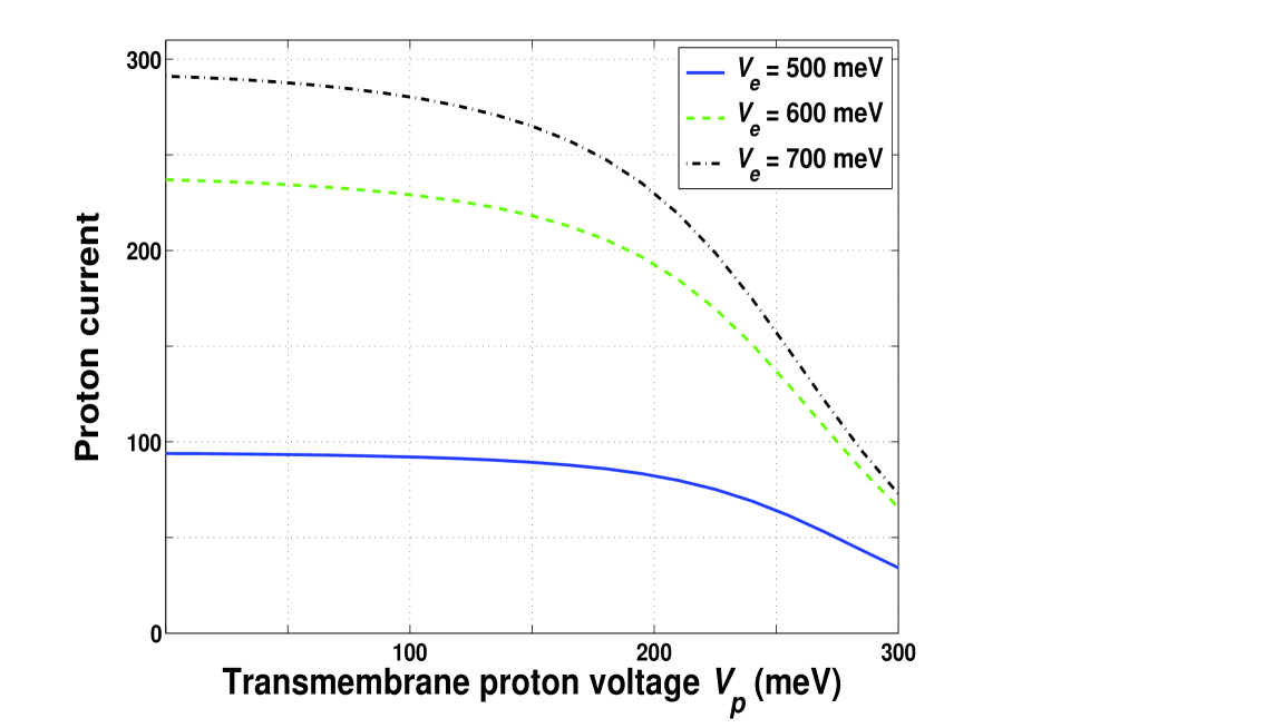
Figure 3: (Color online) Proton current versus transmembrane voltage $V_{p}$ at room temperature, $T=298$ K, and three different electron potentials: $V_{e}=500,\;600,\;$ and $700$ meV. The proton current is almost constant for low values of $V_{p}$, and decreases for increasing $V_{p}$.

In Fig. 3, we show the steady-state proton current $I_{P}$ as a function of the transmembrane voltage gradient $V_{p}$, at three different values of the electron voltage: $V_{e}=500,\;600,\;700$ meV. We use here the standard set of other parameters (see the previous subsection), where $T=298$ K and $\lambda_{e}=\Lambda_{p}=100$ meV.

The proton current $I_{P}$ is equal to the number of protons pumped energetically uphill (at $V_{p}>0$), from the negative side $N$ to the positive side $P$ of the membrane, per one microsecond. At the difference $V_{e}=600$ meV of source and drain redox potentials, the system pumps more than 200 protons per one microsecond against the transmembrane voltage gradient $V_{p}=150$ meV. According to Eq. (53), this voltage corresponds to the proton electrochemical gradient $\Delta\mu_{H}=210$ meV, which is usually applied to the internal membrane of mitochondria and the plasma membranes of bacteria. The number of pumped protons goes down as the proton voltage $V_{p}$ increases, and goes up with increasing the electron voltage difference $V_{e}$. The proton current saturates at $V_{e}>750$ meV. It is evident from Fig. 3 that at high enough electron voltages ($V_{e}\geq 600$ meV), the pump is able to translocate more than 100 protons per microsecond against the proton gradient $V_{p}$, exceeding 250 meV ($\Delta\mu>310$ meV). The quantum yield $QY$ is about one (with a power-conversion efficiency $\eta\simeq 35$%) in the whole region of electron and proton voltages: 500 meV $<V_{e}<800$ meV, 0 $<V_{p}<300$ meV.

III.1.3 Proton current and the quantum yield as functions of temperature

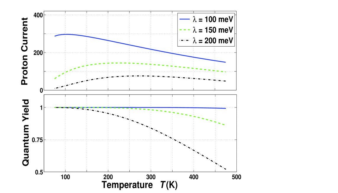
Figure 4: (Color online) Proton current (the number of protons translocated across the membrane per one microsecond) and quantum yield versus temperature for the electron voltage $V_{e}=600$ meV, transmembrane proton voltage $V_{p}=150$ meV, and three different reorganization energies: $\lambda=100,\;150,\;$ and $200$ meV. The proton current and quantum yield both decrease, for increasing $\lambda$.

Figure 4 shows the pumping proton current, $I_{P}$ (i.e., the number of protons translocated from the negative to the positive side of the membrane per one microsecond) versus the temperature $T$ measured in Kelvins. The graphs are presented at three values of the electron and proton reorganization energy: $\lambda=100,\;150,\;200$ meV. We assume here that $\lambda_{e}=\Lambda_{p}=\lambda$, with the electron voltage $V_{e}=600$ meV and the proton gradient $V_{p}=150$ meV. It is of interest that at $\lambda\geq 150$ meV the pumping current has a pronounced maximum near the room temperature, 200 K $<T<300$ K, although the quantum yield is higher, $QY\sim 1$, at lower temperatures. The performance of the pump deteriorates at higher reorganization energies when the coupling to the environment increases. Increasing the reorganization energy leads to increasing the probability for an electron to be transferred through the system, losing all its excess energy to the environment without transferring this energy to protons. Such a probability is further increased at large temperatures leading to the observed decrease of the quantum yield.

III.1.4 Dependence of the proton current on the parameters of the interaction site

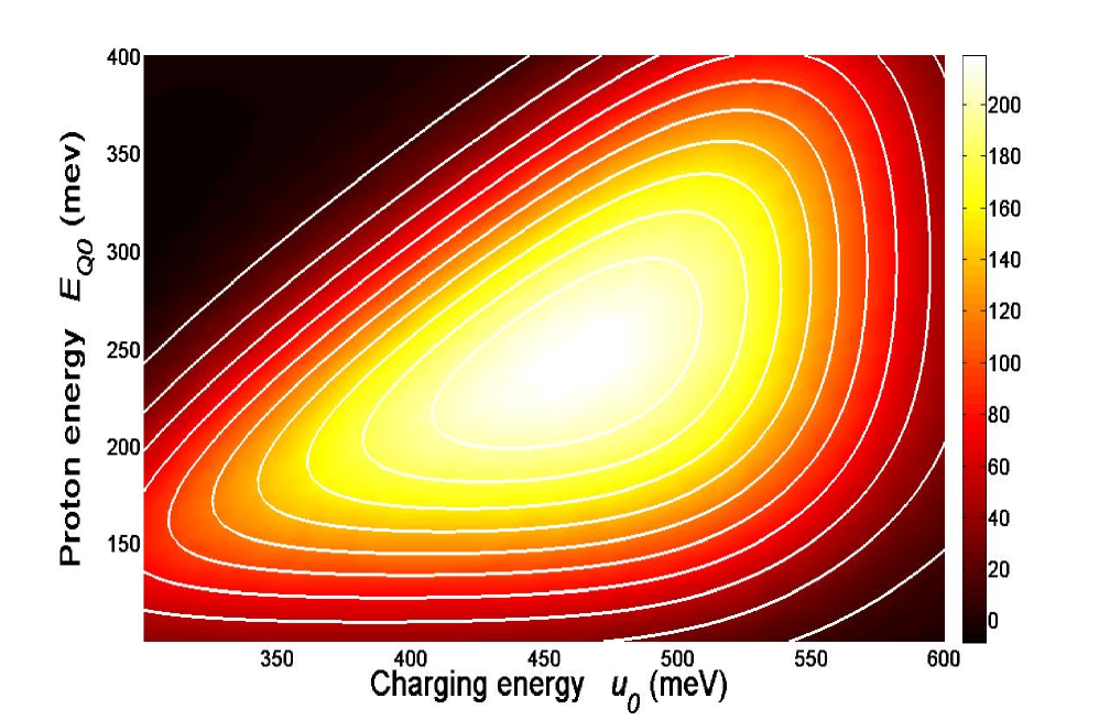
Figure 5: (Color online) Dependence of the proton current (the number of protons pumped across the membrane per one $\mu$s, see the color bar on the right side) on the charging energy $u_{0}$, and on the energy $E_{Q0}$ of the central proton site for $V_{e}=600$ meV, $V_{p}=150$ meV, and $T=298$ K.

The energy transfer from the electron to the proton component occurs on the interaction site $Q=\{Q_{e},Q_{p}\}$, which has one electron ($\varepsilon_{Q}$) and one proton ($E_{Q}$) energy levels (see Eq. (54)). The electron on the site $Q_{e}$ is electrostatically coupled to the proton, which populates the site $Q_{p}$, with the Coulomb energy $u_{0}$. It follows from Fig. 5 that the proton pumping current $I_{P}$ exhibits a resonant behavior as a function of the charging energy $u_{0}$ and the position of the proton energy level $E_{Q0}$. The dependence of the pumping current on the electron energy $\varepsilon_{Q}$ has a resonant character as well. Here we assume that $V_{e}=600$ meV, $V_{p}=150$ meV, $\lambda_{e}=\Lambda_{p}=100$ meV, and $T=298$ K. The energetically-uphill proton current has a pronounced maximum ($I_{P}\simeq 220/\mu$s) at the Coulomb energy $u_{0}=470$ meV and the proton energy $E_{Q0}=250$ meV, provided that the electron energy $\varepsilon_{Q}=-250$ meV. It is important that the proton pump is robust to the variations of the Coulomb energy $u_{0}$ and the proton energy $E_{Q0}$ in the range $\pm 50$ meV from the resonant values. The quantum yield $QY$ is very close to one in the central region of Fig. 5, so that the power-conversion efficiency $\eta$ is about of 35%.

Figures 3, 4 and 5 clearly demonstrate that, at standard physiological conditions, the static redox-linked proton pump (“CcO-pump”) efficiently converts the energy of electrons to the more stable energetic form of the proton electrochemical gradient across the membrane.

III.2 Redox loop mechanism of electron and proton translocation

In many biological systems, electrons and protons can be transferred across a membrane by means of a molecular shuttle diffusing inside of the membrane, from one side to another. Here we show that the mathematical model described in Section II can be successfully applied for a description of the redox loop mechanism, which utilizes the Brownian motion of the shuttle $Q$ carrying both electron, $Q_{e}$, and proton, $Q_{p}$, sites (see Fig. 2). As in the previous case, we have to solve here a system of master equations for the electron ($n_{L},n_{Q},n_{R}$) and proton ($N_{A},N_{Q},N_{B}$) populations, Eqs. (36,37), and for the correlation function $K$ of electron and proton populations on the site $Q$, Eq. (43). However, these master equations should be complemented by the Langevin equation, Eq. (49), for the time-dependent shuttle position $x$. We note that the electron tunneling between the sites $L$-$Q$, $Q$-$R$, as well as the proton transfer rates between the sites $A$-$Q$ and $Q$-$B$, depend on the position $x$ of the shuttle.

III.2.1 Parameters

We assume that the electron site $L$ is located near the negative ($N$) side of the membrane, at $x=-x_{0}$, where $x_{0}=2$ nm. The other electron site $R$ is near the $P$-side of the membrane, at $x=+x_{0}$. The reservoir $S$, connected to the site $L$, serves as a source of electrons, and the reservoir $D$, coupled to the site $R$, serves as an electron drain (see Fig.2). The tunneling amplitudes $\Delta_{L},\Delta_{R}$ are determined by the amplitudes $\Delta_{L0},\;\Delta_{R0}$, and by the electron tunneling length $l_{e}$:

$$\Delta_{L}(x)=\Delta_{L0}\times\exp\left(-\frac{|x+x_{0}|}{l_{e}}\right),$$

$$\Delta_{R}(x)=\Delta_{R0}\times\exp\left(-\frac{|x-x_{0}|}{l_{e}}\right).$$ (56)

The proton-binding site $A$ is located at the end of the $N$-side proton pathway, whereas the site $B$ terminates a pathway, which goes into the $P$-side of the membrane. For the $x$-dependencies of the proton transfer amplitudes $\Delta_{A}$ and $\Delta_{B}$, we choose the following relations:

$$\Delta_{A}(x)=\Delta_{A0}\times\left[\exp\left(\frac{x_{0}+x}{l_{p}}\right)+1\right]^{-2},$$

$$\Delta_{B}(x)=\Delta_{B0}\times\left[\exp\left(\frac{x_{0}-x}{l_{p}}\right)+1\right]^{-2},$$ (57)

where $l_{p}$ is the proton transfer length. It should be noted that our model produces the same results when the proton amplitudes are given by the expressions similar to Eqs. (56). For the transfer parameters, we choose the following values: $\Delta_{L0}\sim\Delta_{R0}=0.04$ meV, $\Delta_{A0}\sim\Delta_{B0}=0.04$ meV, and $l_{e}=0.25$ nm, $l_{p}=0.25$ nm. Couplings to the electron and proton reservoirs are described by the rates $\gamma_{S}\sim\gamma_{D}=0.5/$ns and $\Gamma_{N}\sim\Gamma_{P}=0.1/$ns. The system is robust to significant variations of the transfer parameters.

The confinement potential $U_{c}(x)$ is determined by the height $U_{c}=500$ meV, the steepness $l_{c}=0.1$ nm, and the half-width $x_{c}=2.7$ nm. The potential barrier $U_{s}(x)$, preventing the charged shuttle from entering into the membrane, is characterized by the height $U_{s}=770$ meV, the width $x_{s}=1.7$ nm, and the steepness $l_{s}=0.05$ nm.

Accordingly, the electron and proton populations of the shuttle are almost completely compensated, $n_{Q}\simeq N_{Q}$, so that the potential $U_{s}(x)$ gives a negligible contribution to the energies of electrons and protons. However, we have to take into account the fact that in the presence of the voltage gradient, $V_{p}\simeq 150$ meV, the electron ($\varepsilon_{Q}$) and proton ($E_{Q}$) energies on the moving shuttle depend on the shuttle position $x$:

$$\varepsilon_{Q}=\varepsilon_{Q0}-\frac{x}{2x_{0}}V_{p},$$

$$E_{Q}=E_{Q0}+\frac{x}{2x_{0}}V_{p},$$ (58)

with $\varepsilon_{Q0}=280$ meV, and $E_{Q0}=u_{0}/2=200$ meV, where for the charging energy $u_{0}$ of the shuttle we have: $u_{0}=400$ meV.

Thus, electrons move from the source reservoir, having the electrochemical potential $\mu_{S}=420$ meV, to the $L-$site (with the energy $\varepsilon_{L}=380$ meV), and, thereafter, to the shuttle. On the opposite side of the membrane, the electron, populating the shuttle, jumps to the site $R$ ($\varepsilon_{R}=-170$ meV) and, finally, to the drain reservoir ($\mu_{D}=-230$ eV). The total drop of the redox potential in this electron-transport chain can be estimated as $\mu_{S}-\mu_{D}=650$ meV.

Protons move from the $N$-side of the membrane ($\mu_{N}=-105$ meV) to the site $A$, having a lower energy $E_{A}=-150$ meV. The energy level $E_{Q}=125$ meV of the proton on the shuttle, located near the $N$-side of the membrane (at $x=-x_{0}$), is much higher than $E_{A}$, if the shuttle contains no electrons. However, the shuttle populated with a single electron is more attractive for protons, since in this case the effective energy of the proton, $E_{Q}-u_{0}=-275$ meV, is less than the energy of the proton-binding site $A$. The shuttle, carrying one electron and one proton, diffuses to the opposite side of the membrane ($x=+x_{0}$), where the electron, with energy $\varepsilon_{Q}-u_{0}=-195$ meV, is able to tunnel to the site $R$, having a slightly higher energy $\varepsilon_{R}=-170$ meV. In the absence of an electron, the energy of the proton on the shuttle (at $x=+x_{0}$) increases to the level $E_{Q}=E_{Q0}+V_{p}/2=275$ meV, which exceeds the energy of the proton on the site $B$: $E_{B}=150$ meV. Consequently, the proton moves from the shuttle to the site $B$ and, thereafter, to the $P$-side of the membrane characterized by the electrochemical potential $\mu_{P}=+105$ meV. Thus, this redox loop mechanism translocates protons across the membrane against the proton electrochemical gradient $\Delta\mu_{H}=\mu_{P}-\mu_{N}=210$ meV, and against the transmembrane potential $V_{p}\sim 150$ meV.

III.2.2 Proton translocation process

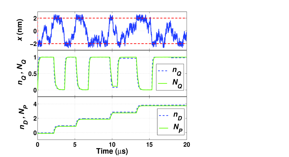
Figure 6: (Color online) Time evolution of the electron-proton translocation process. Here $x$ is the location of the shuttle, $n_{Q}$ and $N_{Q}$ are the electron and proton populations of the shuttle, respectively, $n_{D}$ is the number of electrons transferred from the electron source $S$ to the electron drain $D$, and $N_{P}$ is the number of protons translocated from the negative ($N$) to the positive ($P$) side of the membrane. It can be seen from this figure that the loading/unloading of the shuttle with electrons and protons, as well as the electron and proton transfer across the membrane, are clearly correlated with the spatial motion of the shuttle.

Figure 6 exhibits the electron and proton populations of the shuttle, $n_{Q}(t)$ and $N_{Q}(t)$, correlated with the shuttle’s position $x(t)$ at $T=298$ K, $V_{p}=150$ meV, and at $\Delta\mu=210$ meV. In this figure, we also show the time dependencies of the number of electrons, $n_{D}(t)$, transferred to the drain reservoir, and the number of protons, $N_{P}(t)$, translocated to the positive side of the membrane. The shuttle diffuses between the membrane walls located at $x=\pm x_{0}$ ($x_{0}=2$ nm) with an average crossing time $\Delta t\sim 2.5\,\mu$s. This time-scale is closely related to the diffusion time,

$$t_{D}\sim\langle\Delta x^{2}\rangle/2D\sim 2.66\;\mu{\rm s}\,,$$

obtained at $\sqrt{\langle\Delta x^{2}\rangle}\sim 2x_{0}=4$ nm, for the diffusion coefficient of the quinone molecule $D\sim 3\cdot 10^{-12}\,$m${}^{2}/$sec.

At $t\sim 0$, the shuttle, located at $x\sim-x_{0}$, is loaded with one electron and one proton taken from the negative side of the membrane (see Fig. 2). When $t\sim 2.5\;\mu$s, the shuttle reaches the positive side ($x=+x_{0}=2$ nm) and unloads the electron to the the site $R$ (and later to the drain lead $D$) and the proton to the site $B$, coupled to the $P$-side of the membrane. Consequently, the population $N_{P}$ of the $P$-side grows. The empty shuttle diffuses back, to the $N$-side, completing the cycle, and the process starts again. In twenty microseconds, the shuttle performs four complete trips and translocates about four electrons and four protons across the membrane.

III.2.3 Voltage and temperature dependencies

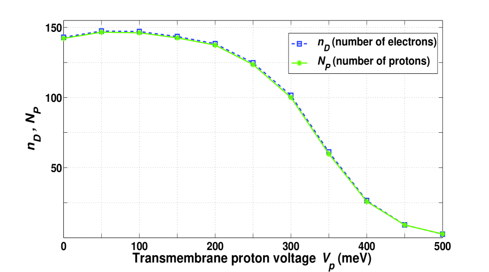
Figure 7: (Color online) Numbers of electrons, $n_{D}$, and protons, $N_{P}$, translocated across the membrane in one millisecond, versus the transmembrane proton voltage $V_{p}$ at room temperature, $T=298$ K, and at $(\mu_{S}-\mu_{D})=650$ meV. Clearly, it is much harder to transfer protons against the higher transmembrane voltages.

The numbers of electrons and protons, $n_{D}$ and $N_{P}$, respectively, transferred across the membrane in one millisecond, are shown in Fig. 7 as functions of the transmembrane proton voltage $V_{p}.$ The electrochemical gradient of protons, $\Delta\mu=\mu_{P}-\mu_{N}$, is proportional to $V_{p}$: $\Delta\mu~{}\simeq~{}V_{p}~{}+~{}60$ meV (at $T=298$ K). The results in Fig. 7 are averaged over ten realizations. The system is able to translocate more than 120 protons per ms against the high transmembrane voltage, $V_{p}\leq 250$ meV, that corresponds to the electrochemical gradient $\Delta\mu\leq 310$ meV.

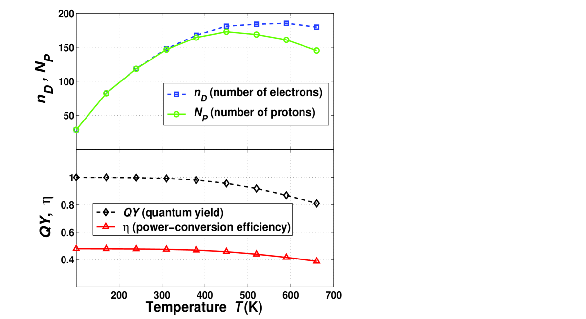
Figure 8: (Color online) Temperature dependence of the numbers of electrons, $n_{D}$, and protons, $N_{P}$, transferred across the membrane by the diffusing shuttle, at $V_{p}=150$ meV and $(\mu_{S}-\mu_{D})=650$ meV. We also present here the quantum yield, $QY$, and the power-conversion efficiency, $\eta$, of the process as functions of the temperature. At higher temperatures, the shuttle moves faster and carries more electrons and more protons. However, if the temperature is too high, the shuttle has not enough time to be loaded with electrons and protons, and sometimes travels empty. As a result of this, the electron and proton currents decrease at high temperatures, thus decreasing the efficiency of the pump.

It follows from Fig. 8 that the translocation mechanism works efficiently in a wide range of temperatures, 250 K $<T<500$ K. In this range, the system pumps more than 120 protons per millisecond with a quantum yield exceeding 90% and with a power-conversion efficiency $\eta$ higher than 40%. With increasing temperature, the shuttle performs more trips between the sides of the membrane, thus, carrying more electrons and protons. This increases the proton current (i.e., the number of protons translocated per unit time). We note that the proton population of the shuttle occurs only after loading the shuttle with an electron. At very high temperatures, $T>500$ K, the shuttle moves quite fast, and protons have less chances to jump on the shuttle. Consequently, the gap between electron and proton currents grows with the temperature, thus deteriorating the performance of the pump.

IV Conclusion

Two different mechanisms of energetically-uphill proton translocation across a biomembrane are described by the same physical model. This model includes three redox sites $(L,Q_{e},R)$ and three proton binding sites $(A,Q_{p},B)$ attached to the source ($S$) and drain ($D$) electron reservoirs, as well as to the proton reservoirs on the positive and negative sides of the membrane. We have shown that it is the strong Coulomb interaction between the electron site $Q_{e}$ and the proton site $Q_{p}$, which plays the most prominent role in the process of energy transformation from electrons to protons. In this case, the whole electron-proton transport chain can be divided into weakly coupled clusters of sites, so that the total number of occupation states is equal to the sum (not to the product) of occupation states in each cluster. At physiological conditions, our model demonstrates a proton pumping effect with a quantum yield near 100% and a power-conversion efficiency of order of 35%, for both the static proton pump, related to the cytochrome c oxidase, as well as for the redox-loop mechanism, where electrons and protons are translocated by the diffusing molecular shuttle.

Acknowledgements. This work was supported in part by the Laboratory of Physical Sciences, National Security Agency, Army Research Office, National Science Foundation grant No. 0726909, JSPS-RFBR contract No. 09-02-92114, Grant-in-Aid for Scientific Research (S), MEXT Kakenhi on Quantum Cybernetics, and Funding Program for Innovative R&D on S&T (FIRST). L.M. was partially supported by the NSF NIRT, Grant No. ECS-0609146 and by the PSC-CUNY Award No. 41-613.

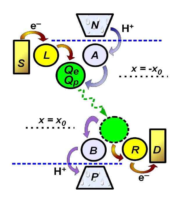
Figure 2: (Color online) Schematic diagram of the redox loop mechanism. Here, the electron-proton interaction site, $Q=\{Q_{e},Q_{p}\}$, is placed on the molecular shuttle (shown in green), which diffuses along the line connecting the negative and positive sides of the membrane. From the source reservoir $S$, an electron ${\rm e}^{-}$ jumps to the site $L$ and, thereafter, to the shuttle, located at $x=-x_{0}.$ The shuttle also accepts a proton ${\rm H}^{+}$ transferred from the $N$-side of the membrane via the site $A$. The loaded shuttle moves randomly toward the positive side ($P$) of the membrane, where (at $x=x_{0}$) the electron is subsequently transferred from the site $Q_{e}$ to the site $R$ and to the drain reservoir $D$, and the proton jumps from the site $Q_{p}$ to the site $B$ and, finally, to the positive ($P$) side of the membrane. We note that, in this design, the electron site $L$ and the proton site $A$ are located near the $N$-side of the membrane (shown by the horizontal blue dashed line), and the electron site $R$ and the proton site $B$ are placed near the $P$-side.

References

- (1) B. Alberts, A. Johnson, J. Lewis, M. Raff, K. Roberts, and P. Walter, Molecular Biology of the Cell (Garland Science, New York, 2002), Ch. 14.
- (2) D.G. Nicholls and S.J. Ferguson, Bioenergetics 3 (Academic Press, London, 2002).
- (3) M. Wikström and M.I. Verkhovsky, Biochim. Biophys. Acta 1767, 1200 (2007).
- (4) I. Belevich, D. A. Bloch, N. Belevich, M. Wikström, and M.I. Verkhovsky, Proc. Natl. Acad. Sci. U.S.A. 104, 2685 (2007).
- (5) Y.C. Kim, M. Wikström, and G. Hummer, Proc. Natl. Acad. Sci. U.S.A. 104, 2169 (2007).
- (6) A. Yu. Smirnov, L. G. Mourokh, and F. Nori, J. Chem. Phys. 130, 235105 (2009).
- (7) P. Mitchell, J. Theor. Biol. 62, 327 (1976).
- (8) M. Jormakka, S. Törnroth, B. Byrne, and S. Iwata, Science 295, 1863 (2002).
- (9) M.G. Bertero, R.A. Rothery, M. Palak, C. Hou, D. Lim, F. Blasco, J.H. Weiner, and N.C. Strynadka, Nat. Struct. Biol. 10, 681 (2003).
- (10) R.B. Gennis, in Biophysical and Structural Aspects of Bioenergetics, edited by M. Wikström (RSC Publishing, Cambridge, 2005).
- (11) A.Yu. Smirnov, S. Savel’ev, and F. Nori, Phys. Rev. E 80, 011916 (2009).
- (12) P. K. Ghosh, A. Yu. Smirnov, and F. Nori, J. Chem. Phys. 131, 035102 (2009).
- (13) A. Yu. Smirnov, L. G. Mourokh, and F. Nori, Phys. Rev. E 77, 011919 (2008).
- (14) J.R. Johansson, L.G. Mourokh, A.Yu. Smirnov, and F. Nori, Phys. Rev. B 77, 035428 (2008).
- (15) D. A. Cherepanov, L.I. Krishtalik, and A. Y. Mulkidjanian, Biophys. J. 80, 1033 (2001).