Microstructure from ferroelastic transitions using strain pseudospin clock models in two and three dimensions: a local mean-field analysis

Abstract

We show how microstructure can arise in first-order ferroelastic structural transitions, in two and three spatial dimensions, through a local meanfield approximation of their pseudospin hamiltonians, that include anisotropic elastic interactions. Such transitions have symmetry-selected physical strains as their $N_{OP}$-component order parameters, with Landau free energies that have a single zero-strain ’austenite’ minimum at high temperatures, and spontaneous-strain ’martensite’ minima of $N_{V}$ structural variants at low temperatures. The total free energy also has gradient terms, and powerlaw anisotropic effective interactions, induced by ’no-dislocation’ St Venant compatibility constraints. In a reduced description, the strains at Landau minima induce temperature-dependent, clock-like $\mathbb{Z}_{N_{V}+1}$ hamiltonians, with $N_{OP}$-component strain-pseudospin vectors ${\vec{S}}$ pointing to $N_{V}+1$ discrete values (including zero). We study elastic texturing in five such first-order structural transitions through a local meanfield approximation of their pseudospin hamiltonians, that include the powerlaw interactions. As a prototype, we consider the two-variant square/rectangle transition, with a one-component, pseudospin taking $N_{V}+1=3$ values of $S=0,\pm 1$, as in a generalized Blume-Capel model. We then consider transitions with two-component ($N_{OP}=2$) pseudospins: the equilateral to centred-rectangle ($N_{V}=3$); the square to oblique polygon ($N_{V}=4$); the triangle to oblique ($N_{V}=6$) transitions; and finally the 3D cubic to tetragonal transition ($N_{V}=3$). The local meanfield solutions in 2D and 3D yield oriented domain-walls patterns as from continuous-variable strain dynamics, showing the discrete-variable models capture the essential ferroelastic texturings. Other related hamiltonians illustrate that structural-transitions in materials science can be the source of interesting spin models in statistical mechanics.

I Introduction

Ferroelastic crystals undergo diffusionless structural transitions that are first order, and on cooling show a reduction in symmetry to two or more spontaneously-strained states (or ’variants’) which can be transformed between one another by stress R1 ; R2 . These transitions are often studied through minimizing the Landau free energies R3 in terms of appropriate continuous variables, such as displacements, phase fields, or strains R4 ; R5 ; R6 ; R7 . Although homogeneous, single-variant martensite states are the global minimum, elastic heterogeneities or metastable domain-wall patterns are experimentally found R8 , that are locked in to preferred crystallographic directions R9 . This orientation arises through a balance between the Landau energies nonlinear in the order parameter strain, the short-range gradient costs or Ginzburg energies, and the effectively long-range elastic energies R10 or powerlaw anisotropic interactions, that orient the domain walls  R5 ; R7 ; R10 . The powerlaw interactions result from enforcing St Venant ’compatibility’ constraints R11 ; R12 between the strain components so that the displacements are continuous, with no dislocations generated on cooling. Continuous-variable models have been used to study microstructures under various conditions, including strain-rate dependence R13 ; and the effects of finite-size on martensitic growth in an austenitic matrix  R14 .

Models in terms of discrete structure-variables or ’pseudospins’ have also been used to study these ferroelastic transitions R15 ; R16 . (Similar in spirit to discrete strains, analytic ‘minimizing sequences’ consider tent-like displacement profiles or flat strain-variants, on either sides of domain walls R2 .) Recently, model pseudospin hamiltonians induced by the scaled free energies for several specific transitions in 2D and 3D have been proposed R17 . The model hamiltonian is simply the total scaled R18 free energy evaluated at the Landau minima in the order parameters (OP). The pseudospins are ’arrows’ in $N_{OP}$-dimensional order-parameter space, pointing to the $N_{V}$ variant minima, and to the zero-strain turning point. The hamiltonian includes a temperature-dependent on-site term quadratic in the pseudospins from the Landau term, a nearest-neighbor ferromagnetic interaction between pseudospins from the Ginzburg term, and a pseudospin powerlaw interaction from the St Venant term. The pseudo-spin models are like $\mathbb{Z}_{N_{V}+1}$ clock models R19 generalized to include a spin-zero state, and may be termed ’clock-zero’ models R17 . A three-state spin-1 type model for the transition of square to rectangle unit cells (with $N_{OP}=1,N_{V}=2$) has found glass-like behavior on slow cooling using a local meanfield approximation R17 .

In this work we consider pseudo-spin models in the local meanfield approximation under temperature quenches, for five structural transitions : four in two spatial dimensions R20 , and one in three spatial dimensions R7 . Apart from the single order parameter ($N_{OP}=1$) square/rectangle case that is first studied as a simple prototype, the other four transitions all have two-component ($N_{OP}=2$) pseudospins. The transitions are i) the square to rectangle (2D version of the tetragonal/orthorhombic transition such as in YBCO); ii) the square to oblique polygon; iii) the triangle to centred-rectangle (2D version of hexagonal to orthorhombic transition such as in lead orthovanadate R4 ; R6 ; R7 ); iv) the triangle to oblique; and v) in 3D, the cubic to tetragonal transition (as in FePd). For these five transitions, the (nonzero) pseudospin arrows point respectively, to the two ends of a line, and to the corners of a square, a triangle, a hexagon, and a triangle, with the number of pseudospin variant states thus being respectively $N_{V}=2,4,3,6$ and $3$. We show that these discrete-variable models, despite their simplicity, produce local-meanfield microstructure in one- and two-component strain pseudospins in agreement with continuous-variable strain simulations R4 ; R5 ; R6 ; R7 , that can be computationally more intensive. We thus find parallel twins for the square/rectangle and cubic/tetragonal transitions; nested stars for the equilateral/isosceles triangle transition; and tilted oblique domains for the square/oblique, and triangle/oblique transitions.

The generalized clock model of strain pseudospins is a statistical mechanics description of the ferroelastic transitions in materials science. It conceptually links long-lived, metastable martensitic twins (even without quenched disorder) to Potts-model and clock-model descriptions of glasses R19 , and may be relevant to recent quenched-disorder strain glass behavior in martensitic alloys R21 .

The plan of the paper is as follows. In Section II we outline the derivation R17 of the pseudospin hamiltonians, and of compatibility potentials for the four 2D transitions. Our meanfield microstructure results are in Section III where we first consider the two-variant square/rectangle case as a prototype, its response to external stress, and its relation to the spin-1 Blume-Capel model R21 . We then consider local meanfield microstructure for the three-variant triangle to centred-rectangle transition; the four-variant square/oblique transition; and the six-variant triangle/oblique transition. Turning to 3D, Section IV considers the local meanfield microstructure for the three-variant cubic/tetragonal transition, with its compatibility potential stated in the Appendix. In Section V we mention other related spin models of interest in statistical mechanics. The final Section  VI has a summary and conclusion.

II PSEUDOSPIN HAMILTONIANS IN TWO SPATIAL DIMENSIONS

The free energy functionals describing ferroelastic structural transitions can be written in terms of the physical strains, that are symmetry-specific linear combinations of the Cartesian strain-tensor components. The Landau terms are invariant polynomials of the $N_{OP}$ order parameter strains, and have $N_{V}$ minima. The free energies have many material-dependent elastic coefficients, that are not always known, or are fitted to experiment only for specific materials. However, the spontaneous order-parameter strain magnitude at the first-order transition temperature is a small parameter. Following Barsch and Krumhansl R18 a scaling procedure has been applied R17 to four 3D transitions and five 2D transitions to obtain scaled Landau free energies that (to leading order in the small parameter) show universality at their minima, where any internal elastic constants are scaled out, and material dependence is only in an overall elastic-energy prefactor. ‘Geometric nonlinearities‘ are higher order in the spontaneous strain and are neglected, as a perturbative first approximation. Then different materials with the same transition, fall into the same ’quasi-universality’ class, with common behaviour at the scaled minima, that lie at the corners and centres of the same ’polyhedron’ in $N_{OP}$ dimensional order parameter space. This is useful in strain-variable dynamics. It also immediately suggests a reduced description of ferroelastics, in terms of discrete-strain statistical variables or vector ’pseudospins’, directed to these minima.

A specific reduction procedure was proposed R17 to obtain pseudospin hamiltonians by evaluating scaled free energies evaluated at their Landau minima. The basic idea is quite simple. i) Scale the total free energy to dimensionless form, including the specifically calculated compatibility-induced powerlaw interaction term, and the gradient term. Write the Landau free energy in polar coordinates in OP space, with the austenite minimum at the origin, and $N_{V}$ martensite minima located on a circle in $N_{V}$ discrete angular directions. ii) Set the radial OP-magnitude to its common temperature-dependent Landau-minimum value, and replace the OP-minima directional angles by discrete vectors pointing to these $N_{V}+1$ minima on the circle, and at the centre.
iii) The total free energy evaluated at minima is then the model Hamiltonian for the vector pseudospins, that have $N_{OP}$ spin-components, and $N_{V}+1$ values. The remaining model coefficients are then not just arbitrary, but are related through the parent free energy, to the scaled temperature, to the scaled energy cost of an elastic domain-wall segment, and to the scaled bulk stiffness.

We outline below the derivation R17 of the pseudospin hamiltonians and compatibility potentials in two spatial dimensions, for the square/rectangle, triangle/ /centred-rectangle, square/oblique, and triangle/oblique transitions, with number of variants $N_{V}=2,3,4$ and $6$ respectively. The 3D case is considered later.

II.1 Square to Rectangle (SR) hamiltonian: $N_{OP}=1,N_{V}=2$

Consider the prototypical square-to-rectangle or ’SR’ transition, that is a two-dimensional analog of a tetragonal to orthorhombic transition. For small distortions, the components of the symmetric Cartesian strain tensor are given by $e_{\mu\nu}=1/2\ (\partial_{\mu}u_{\nu}+\partial_{\nu}u_{\mu})$, where $\vec{u}(\vec{r})$ is the displacement vector and $\mu,\nu=x,y$. We define linear combinations of the Cartesian components as three physical strains, describing compressional ($e_{1}$), deviatoric ($e_{2}$) and shear ($e_{3}$) distortions.

$$e_{1}=\frac{c_{1}}{2}\ (e_{xx}+e_{yy}),\ \ e_{2}=\frac{c_{2}}{2}\ (e_{xx}-e_{yy}),\ \ e_{3}=\frac{c_{3}}{2}(e_{xy}+e_{yx}),$$ (1)

where $c_{1}$, $c_{2}$ and $c_{3}$ are symmetry-specific constants R7 . For the square reference lattice, $c_{1}=c_{2}=\sqrt{2}$ and $c_{3}=1$. For the equilateral triangle reference lattice $c_{1}=c_{2}=c_{3}=1$. The pseudospin hamiltonian is obtained by the three steps given above, that we follow for all transitions.

i) Scaled free energy, and compatibility potential :

For the SR case, the deviatoric strain $e_{2}$ is the order parameter (OP). The compressional and shear strains are the non-OP strains. The scaled free energy is $F=E_{0}{\bar{F}}$ where the overall $E_{0}$ is an elastic energy per unit cell, and the dimensionless $\bar{F}=\bar{F}_{L}+\bar{F}_{G}+\bar{F}_{non}$ is a sum of three terms,

$$\bar{F}_{L}=\sum_{\vec{r}}{\bar{f}}_{L}(e_{2});~{}\bar{F}_{G}=\sum_{\vec{r}}{\bar{f}}_{G}(\vec{\nabla}e_{2});~{}\bar{F}_{non}=\sum_{\vec{r}}{\bar{f}}_{non}(e_{1},e_{3}).$$ (2)

where $\sum_{\vec{r}}\rightarrow\int d^{2}r/a_{0}^{2}$ runs over all positions, and $a_{0}$ is a lattice scale for a computational grid.

The dimensionless, scaled Landau free energy density in coordinate space is sixth order in $e_{2}(\vec{r})$ to give a first order transition R5 ; R7 ,

$${\bar{f}}_{L}(e_{2})=(\tau-1)e_{2}^{2}+e_{2}^{2}(e_{2}^{2}-1)^{2}.$$ (3)

A scaled temperature is defined by

$${\tau\equiv(T-T_{c})/(T_{0}-T_{c}).}$$ (4)

There can be three $\partial f_{L}/\partial e_{2}=0$ minima: at zero-strain $e_{2}=0$ austenite, and at two martensite variant minima of nonzero strain, $e_{2}=\pm\bar{\varepsilon}(\tau)$. The order-parameter magnitude $\bar{\varepsilon}$ at the variant minima is

$${{\bar{\varepsilon}}(\tau)=[\frac{2}{3}(1+\sqrt{1-3\tau/4})]^{1/2}.}$$ (5)

On cooling below the upper spinodal $\tau=4/3$, two martensite variants appear ; they become degenerate with the austenite zero-state at $\tau=1$ or $T=T_{0}$ when ${\bar{\varepsilon}}(\tau=1)=1$; and for $\tau<1$ the martensite wells become lower in energy. The austenite minimum disappears below the lower spinodal $\tau=0$ or $T=T_{c}$.

The cost of creating interfaces or domain walls is given by the usual Ginzburg term, with $\xi$ a wall thickness scale,

$${\bar{F}_{G}=\sum_{\vec{r}}\xi^{2}({\vec{\nabla}}e_{2}(\vec{r}))^{2}=\sum_{\vec{k}}\xi^{2}{\vec{k}}^{2}|e_{2}(\vec{k})|^{2}.}$$ (6)

Finally, the non-OP strain energy is simply harmonic in compressional ($e_{1}$) and shear ($e_{3}$) strains,

$${\bar{F}_{non}=\sum_{{\vec{r}},i=1,3}\frac{1}{2}A_{i}{e_{i}(\vec{r})}^{2}=\sum_{{\vec{k}},i=1,3}\frac{1}{2}A_{i}|e_{i}(\vec{k})|^{2}.}$$ (7)

The scaled compressional and shear elastic constants can be expressed in terms of the (unscaled) elastic constants $C_{ij}$ in the Voigt notation, evaluated at $T_{0}$. For the cubic case R17 , $A_{1}=(C_{11}+2C_{12})/(C_{11}-C_{12})$. The ratio $A_{1}/A_{3}$ is taken as fixed in simulations, for simplicity.

For $\vec{k}=0$ uniform contributions, the optimum non-OP strains are zero, at the parabolic $f_{non}=0$ minimum. For spatially varying $\vec{k}\neq 0$ contributions, the non-OP strains are to be minimized subject to the St Venant compatibility constraint R5 ; R7 ; R11 ; R12 that says distorted unit cells fit together in a smoothly compatible fashion, without defects like dislocations, so the displacement field is single-valued. The St. Venant conditions in the Cartesian strain tensor ${\bf e}$ are  R11 ; R12 (with ’ T ’ a transpose),

$${{\vec{\nabla}}\times({\vec{\nabla}}\times{\bf e})^{T}=0.}$$ (8)

In two dimensions, the constraint in terms of physical strains of (1) is

$${\frac{1}{c_{1}}{\vec{\nabla}}^{2}e_{1}-\frac{1}{c_{2}}(\partial^{2}_{x}-\partial^{2}_{y})e_{2}-\frac{2}{c_{3}}\partial_{x}\partial_{y}e_{3}=0.}$$ (9)

or in Fourier space

$${O_{1}e_{1}(\vec{k})+O_{2}e_{2}(\vec{k})+O_{3}e_{3}(\vec{k})=0,}$$ (10)

where the compatibility coefficients are

$${O_{1}=\frac{-\vec{k}^{2}}{c_{1}}},\ \ \displaystyle{O_{2}=\frac{k_{x}^{2}-k_{y}^{2}}{c_{2}}},\ \ \displaystyle{O_{3}=\frac{2k_{x}k_{y}}{c_{3}}}.$$ (11)

The constrained minimization can be done through Lagrange multipliers R5 , or by a direct substitution of the constrained solution R17 $e_{1}=-(O_{2}e_{2}+O_{3}e_{3})/O_{1}$ of (10), into the non-OP free energy of (7),

$${\bar{f}_{non}=\sum_{\vec{k}\neq 0}\frac{1}{2}\left[A_{1}~{}|(O_{2}e_{2}+O_{3}e_{3})/O_{1}|^{2}+A_{3}|e_{3}|^{2}\right].}$$ (12)

A free minimization in the remaining non-OP strain $e_{3}$ determines it in terms of the OP $e_{2}$. In fact, $e_{i}=-(O_{i}O_{2}/A_{i})/[(O_{1}^{2}/A_{1})+(O_{3}^{2}/A_{3})]$ for $i=1,3$. Substituting into (7) yields the compatibility-induced interaction $\bar{F}_{compat}(e_{2})\equiv\bar{F}_{non}(e_{1},e_{3})$, where

$${\bar{F}_{compat}=\sum_{\vec{k}}\frac{A_{1}}{2}U(\vec{k})|e_{2}(\vec{k})|^{2}}.$$ (13)

The compatibility kernel $U$ in Fourier space is

$${A_{1}U(\vec{k})=\nu(\vec{k})\dfrac{O_{2}^{2}}{[(O_{1}^{2}/A_{1})+(O_{3}^{2}/A_{3})]}},$$ (14)

or explicitly from (11), and $c_{1}=c_{2}=\sqrt{2},c_{3}=1$,

$${U(\vec{k})=\nu(\vec{k})\dfrac{(k_{x}^{2}-k_{y}^{2})^{2}}{k^{4}+8\frac{A_{1}}{A_{3}}k_{x}^{2}k_{y}^{2}}}.$$ (15)

Here the prefactor $\nu(\vec{k})\equiv 1-\delta_{{\vec{k}},0}$ is inserted to make $f_{non}\sim U$ vanish for $\vec{k}=0$ uniform non-OP strains, as mentioned. In coordinate space, this is a powerlaw interaction between OP strains $U(\vec{R})\sim 1/R^{d}$, with sign-variation in angular directions yielding zero angular average ($\sum_{\vec{R}}U(\vec{R})\sim U(\vec{k}=0)=0$), so it is not ’long-range’ in the isotropic Coulomb $\sim 1/R^{d-2}$ sense. The powerlaw anisotropic interactions are easily evaluated in Fourier space, and one need not resort to uncontrolled coordinate-space truncations to near-neighbor couplings, that may leave out some essential physics of the transition. In coordinate space,

$${\bar{F}_{compat}(e_{2})=\frac{1}{2}\sum_{{\vec{r}},{\vec{r}^{\prime}}}A_{1}U(\vec{r}-\vec{r}^{\prime})e_{2}(\vec{r})e_{2}(\vec{r}^{\prime})}.$$ (16)

The formal partition function

$${Z=\int\prod_{\vec{r}}de_{2}(\vec{r})\exp(-\beta F[e_{2}(\vec{r})])},$$ (17)

is dominated by free energy textural minima, that may be asymptotically found in a TDGL or relaxational dynamics, as done elsewhere R7 ,

$${\frac{\partial e_{2}(\vec{r},t)}{\partial t}=-\frac{\delta F}{\delta e_{2}(\vec{r},t)}}.$$ (18)

ii) Continuous strains to discrete pseudospins :

One can approximate the partition function by retaining only the Landau-minima at fixed OP-magnitude values $|e_{2}|=\bar{\varepsilon}(\tau)$, and different OP signs (or in general, different angular directions of minima), while neglecting fluctuations about these minima. The continuous-variable strains are then replaced by discrete-variable pseudospins R17

$${e_{2}(\vec{r})\rightarrow{\bar{\varepsilon}}(\tau)S(\vec{r})},$$ (19)

where the pseudospin has the three values $S(\vec{r})=0,\pm 1$, to locate the minima at $e_{2}=0,\pm{\bar{\varepsilon}}(\tau)$. Although in zero stress the uniform austenite state is no longer a Landau minimum below the lower spinodal $\tau=0$, the surrounding nonuniform textures can exert local internal stresses to locally favor the zero value, even at low temperatures. Also, the free energy in OP strain always has a turning point at the origin to support dynamical transient zeros, that although few in number, could play a catalytic role in microstructural evolution R17 . Hence we retain zero spin values at all temperatures, allowing their permanent/transient existence to be determined dynamically.

With this substitution and $S^{6}=S^{4}=S^{2}=1,0$, the approximated Landau free energy density at the minima can be written as R17

$${{\bar{f}}_{L}={\bar{\varepsilon}}^{2}(\tau)g_{L}(\tau)S^{2}(\vec{r});~{}~{}g_{L}\equiv(\tau-1)+({\bar{\varepsilon}}^{2}-1)^{2}.}$$ (20)

where $\bar{\varepsilon}$ is in (5).

iii) The reduced pseudospin hamiltonian :

The partition function of (17) reduces to a sum over all the pseudospin configurations, with a temperature-dependent effective Hamiltonian in the Boltzmann weight, that can then be studied by the usual methods of statistical mechanics. Substituting (19) into the total scaled free energy directly yields the hamiltonian in coordinate space,

$${H(S)\equiv{\bar{F}}(e_{2}\rightarrow\bar{\varepsilon}S)},$$ (21)

where

$$\displaystyle\beta H(S) =\frac{D_{0}}{2}[\sum_{\vec{r}}\{g_{L}S^{2}(\vec{r})+\xi^{2}(\vec{\nabla}S)^{2}\}$$ (22)

$$+\sum_{{\vec{r}},{\vec{r}^{\prime}}}\frac{A_{1}}{2}U({\vec{r}}-{\vec{r}^{\prime}})S(\vec{r})S(\vec{r}^{\prime})],$$

and $D_{0}\equiv 2E_{0}\bar{\varepsilon}(\tau)^{2}/T$. This has the form of a generalized spin-1 Blume-Capel model R22 as discussed later, but with temperature-dependent coefficients and powerlaw interactions. The hamiltonian is diagonal in Fourier space R17 ,

$${\beta H=\frac{1}{2}\sum_{\vec{k}}Q_{0}(\vec{k})|S(\vec{k})|^{2}},$$ (23)

where

$${Q_{0}(\vec{k})\equiv D_{0}[g_{L}(\tau)+\xi^{2}{\vec{k}}^{2}+\frac{A_{1}}{2}U(\vec{k})]}.$$ (24)

II.2 Triangle/Centred Rectangle (TCR) hamiltonian: $N_{OP}=2,N_{V}=3$

Consider a two-dimensional crystal with equilateral triangles transforming to isosceles triangles, with three possible such variants ($N_{V}=3$), as there are three sides that can become the unequal side. The unit-cell changes from an equilateral triangle to a centred-rectangle. This ’TCR’ transition is the 2D version of the hexagonal to orthorhombic transition observed in lead orthovanadate R8 . There are two order parameters R4 ; R7 ; R17 ; R20 : the deviatoric strain $e_{2}$, and the shear strain $e_{3}$. The single non-OP variable is the bulk dilatation or compressional strain $e_{1}$. Just like this TCR case, the square/oblique, triangle/oblique and cubic/tetragonal transitions also have the same OP $(e_{2},e_{3})$ and a single non-OP strain $e_{1}$, but of course are distinguished by their different, transition-specific Landau polynomials, that induce different $N_{V}$ directions of the vector pseudospins.

i) Scaled free energy and compatibility potential :

The free energy functional, invariant under the triangular point group symmetry, is

$${\bar{F}=\sum_{\vec{r}}\left\{{\bar{f}}_{L}\left(e_{2},e_{3}\right)+{\bar{f}}_{G}\left({\vec{\nabla}}e_{2},{\vec{\nabla}}e_{3}\right)+{\bar{f}}_{non}\left(e_{1}\right)\right\}}.$$ (25)

The Landau free energy $f_{L}$ for the TCR case describes the first-order phase transition between the single high-symmetry austenite phase and the $N_{V}=3$ martensite variants. It has a third-order term invariant under equilateral triangle symmetries, $I_{3}\equiv e_{2}^{3}-3e_{2}e_{3}^{2}$. In scaled form, in coordinate space

$${{\bar{f}}_{L}(e_{2},e_{3})=\tau(e_{2}^{2}+e_{3}^{2})-2(e_{2}^{3}-3e_{2}e_{3}^{2})+(e_{2}^{2}+e_{3}^{2})^{2}.}$$ (26)

Figure 1 shows the Landau free energy with three variant minima, for a low temperature.

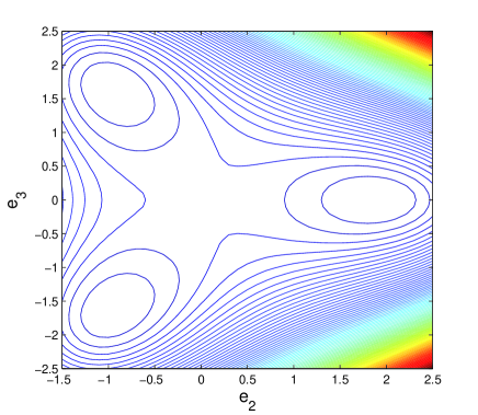
Figure 1: Contour plot in $(e_{2},e_{3})$ space of the Landau free energy for the Triangle to Centred-Rectangle (TCR) transition, with parameters $\tau=-2.5$ and $E_{0}=1$. The three degenerate energy minima correspond to the three martensite variants at this low temperature.

In polar coordinates in OP space, the order parameter vector is $\vec{e}(\vec{r})=(e_{2},e_{3})=\varepsilon(\cos\phi,\sin\phi)$ with magnitude $\varepsilon(\vec{r})\equiv(e_{2}^{2}+e_{3}^{2})^{1/2}$. The Landau free energy in polar coordinates, with $\eta_{3}\equiv\cos 3\phi$ is R17

$${{\bar{f}}_{L}(\varepsilon,\phi)=[(\tau-1)\varepsilon^{2}+\varepsilon^{2}(\varepsilon-1)^{2}]+2(1-\eta_{3})\varepsilon^{3}}$$ (27)

The angular dependence is ${\bar{f}}_{L}\sim-\cos 3\phi$. The minimum conditions $\partial f_{L}/\partial\varepsilon=0;\partial f_{L}/\partial\phi=0$ yield four minima: at the $\vec{e}=0$ austenite, and the three variant minima with $\sin 3\phi=0$ where $\phi=\phi_{m}=0,\pi/3,2\pi/3$, so the last term in (27) vanishes. The three variant minima in the $(e_{2},e_{3})$ plane form a triangle lying on a circle of radius $\varepsilon=\bar{\varepsilon}(\tau)$, where

$${\bar{\varepsilon}(\tau)=\frac{3}{4}(1+\sqrt{1-8\tau/9})}.$$ (28)

On cooling below the upper spinodal $\tau=4/3$, two martensite variants appear ; they become degenerate with the austenite zero-state at $\tau=1$ or $T=T_{0}$ when ${\bar{\varepsilon}}(\tau=1)=1$; and for $\tau<1$ the martensite wells become lower in energy. The austenite minimum disappears below the lower spinodal $\tau=0$ or $T=T_{c}$.

The Ginzburg term ${\bar{f}}_{G}$ is quadratic in the OP-strain gradient so

$${{\bar{F}}_{G}=\sum_{{\vec{r}},\ell=2,3}\xi^{2}({\vec{\nabla}}e_{\ell})^{2}=\sum_{{\vec{k}},\ell=2,3}\xi^{2}{\vec{k}}^{2}|e_{\ell}(\vec{k})|^{2}}.$$ (29)

Finally, the non-OP term is simply harmonic in the single non-OP compressional strain,

$${\bar{F}_{non}(e_{1})=\frac{A_{1}}{2}\sum_{\vec{r}}e_{1}^{2}(\vec{r})=\frac{A_{1}}{2}\sum_{\vec{k}}|e_{1}(\vec{k})|^{2}}.$$ (30)

Substitution of the compatibility solution $e_{1}(\vec{k})=-(O_{2}e_{2}+O_{3}e_{3})/O_{1}$ as for (12) immediately yields the St Venant term $\bar{F}_{compat}(e_{2},e_{3})\equiv{\bar{F}}_{non}(e_{1})$ in terms of the OP,

$${\bar{F}_{compat}=\sum_{\vec{k},\ell,\ell^{\prime}=2,3}\frac{A_{1}}{2}U_{\ell\ell^{\prime}}(\vec{k})e_{\ell}(\vec{k})e_{\ell^{\prime}}(\vec{k})^{*}}.$$ (31)

The compatibility potential kernel is R7 ; R15

$${U_{\ell\ell^{\prime}}=\nu(\vec{k})O_{\ell}O_{\ell^{\prime}}/O_{1}^{2}},$$ (32)

or explicitly from (11) with $c_{1}=c_{2}=c_{3}=1$,

$$U_{22}=\nu\frac{(k_{x}^{2}-k_{y}^{2})^{2}}{k^{4}};~{}U_{22}=\nu\frac{(2k_{x}k_{y})^{2}}{k^{4}};$$

$$U_{23}=\nu\frac{2k_{x}k_{y}(k_{x}^{2}-k_{y}^{2})}{k^{4}}=U_{32}.$$ (33)

In coordinate space,

$${\bar{F}_{compat}(e_{2},e_{3})=\frac{A_{1}}{2}\sum_{\vec{r},\vec{r}^{\prime}}\sum_{\ell,\ell^{\prime}=2,3}U_{\ell\ell^{\prime}}(\vec{r}-\vec{r}^{\prime})e_{\ell}(\vec{r})e_{\ell^{\prime}}(\vec{r}^{\prime})},$$ (34)

and as before, the powerlaw potentials fall off in 2D as $U_{\ell\ell^{\prime}}\sim 1/R^{2}$.

ii) Continuous strains to discrete pseudospins :

For the TCR case (and other two-component OP cases), $N_{V}\geq 3$, but we do not simply get a generalized spin-$j$ model with $2j+1$ states on a line, and $j=N_{V}/2$. Instead we obtain clock-like models R17 ; R19 with discrete $\vec{S}$ vector variables pointing to the polyhedron$N_{V}$ corners and centre, in $N_{OP}$-dimensional space. Since the zero state is included, these may be termed ’clock-zero’ ${\mathbb{Z}}_{N_{V}+1}$ models R17 . Note that, unlike pure clock ${\mathbb{Z}}_{N}$ models R17 , the squared spin $\vec{S}(\vec{r})^{2}=1,0$ is still a statistical variable and not a constant, because of the zero states.

The continuous-variable strains at minima are replaced by discrete-valued pseudospins R17 ,

$${\vec{e}(\vec{r})=\begin{pmatrix}e_{2}\\ e_{3}\end{pmatrix}\longrightarrow\bar{\varepsilon}(\tau)\begin{pmatrix}S_{2}(\vec{r})\\ S_{3}(\vec{r})\end{pmatrix}},$$ (35)

where the two components of the pseudospin have three variant values as in Fig 1 plus zero,

$${\vec{S}=\begin{pmatrix}0\\ 0\end{pmatrix},\begin{pmatrix}1\\ 0\end{pmatrix},\begin{pmatrix}-\frac{1}{2}\\ \pm\frac{\sqrt{3}}{2}\end{pmatrix}}.$$ (36)

For the $N_{V}=3$ variants, $\vec{S}=(\cos\phi_{m},\sin\phi_{m})$ and ${\vec{S}}^{2}=1$, with $\phi_{m}=2\pi(m-1)/3$ and $m=1,2,3$.

With this substitution and ${\vec{S}}^{6}={\vec{S}}^{4}={\vec{S}}^{2}=0,1$, the Landau polynomials again collapse into a simple form, bilinear in the pseudospins,

$${{\bar{f}}_{L}(\tau)=\bar{\varepsilon}^{2}g_{L}{\vec{S}}^{2};~{}~{}g_{L}(\tau)\equiv\tau-1+(\bar{\varepsilon}-1)^{2}},$$ (37)

with $\bar{\varepsilon}$ as in (28).

iii) The reduced pseudospin hamiltonian :

In coordinate space the total pseudospin hamiltonian is

$$\begin{array}[]{rr}\beta H&=\dfrac{D_{0}}{2}[\sum_{\vec{r}}\sum_{\ell=2,3}\{g_{L}{S_{\ell}}(\vec{r})^{2}+\xi^{2}|\vec{\nabla}S_{\ell}(\vec{r})|^{2}\}\\ &+\dfrac{A_{1}}{2}\sum_{\vec{r},\vec{r}^{\prime}}\sum_{\ell,\ell^{\prime}=2,3}U_{\ell\ell^{\prime}}(\vec{r}-\vec{r}^{\prime})S_{\ell}(\vec{r})S_{\ell^{\prime}}(\vec{r}^{\prime})],\end{array}$$ (38)

and is a clock-zero $\mathbb{Z}_{3+1}$ model R17 , with $\vec{S}$ having $3+1$ values of (36), and with a compatibility kernel of (33). It is again diagonal in Fourier space,

$${\beta H=\frac{1}{2}\sum_{\vec{k}}\sum_{\ell,\ell^{\prime}}Q_{0,\ell\ell^{\prime}}(\vec{k})S_{\ell}(\vec{k})S_{\ell^{\prime}}(\vec{k})^{*}},$$ (39)

with $\vec{S}(\vec{k})^{*}=\vec{S}(-\vec{k})$, as ${\vec{S}}(\vec{r})$ is real. Here

$${Q_{0,\ell\ell^{\prime}}(\vec{k})\equiv D_{0}[\{g_{L}(\tau)+\xi^{2}{\vec{k}}^{2}\}\delta_{\ell,\ell^{\prime}}+\frac{A_{1}}{2}U_{\ell\ell^{\prime}}({\vec{k}})].}$$ (40)

II.3 Square/Oblique (SO) hamiltonian: $N_{OP}=2,N_{V}=4$

We consider the square/oblique or ’ SO ’ transition where the transition is driven independently by the deviatoric $e_{2}$ and shear $e_{3}$ order parameter strains R7 ; R17 ; R20 , as modified by a sufficiently strong coupling term.

i) Scaled free energy, and compatibility potential :

The Landau term has the scaled form

$${{\bar{f}}_{L}=\tau(e_{2}^{2}+e_{3}^{2})-(4-C^{\prime}_{4}/2)(e_{2}^{4}+e_{3}^{4})+4(e_{2}^{6}+e_{3}^{6})-C^{\prime}_{4}e_{2}^{2}e_{3}^{2}},$$ (41)

where $C^{\prime}_{4}$ is a material-dependent elastic constant. In polar coordinates, with $\vec{e}=(e_{2},e_{3})=\varepsilon(\cos\phi,\sin\phi)$, it is R17

$${\bar{f}_{L}=[(\tau-1)\varepsilon^{2}+\varepsilon^{2}(\varepsilon^{2}-1)^{2}]+\varepsilon^{4}(3\varepsilon^{2}-2+C^{\prime}_{4}/2)\cos^{2}2\phi}.$$ (42)

The angular dependence is ${\bar{f}}_{L}\sim\cos 4\phi$. The five minima from $\partial{\bar{f}}_{L}/\partial\varepsilon=0;\partial{\bar{f}}_{L}/\partial\phi=0$ are the austenite zero state, and four variant minima with $\sin 4\phi=0$ in angular directions $\phi=\phi_{m}=\pi(2m-1)/4$ with $m=1,2,3,4$. The last term in (42) vanishes at minima, suppressing the $C_{4}^{\prime}$ material dependence. The four variant minima in the $e_{2},e_{3}$ plane for $\tau<4/3$ form a square lying on a circle of radius $\varepsilon=\bar{\varepsilon}(\tau)$, where $\bar{\varepsilon}$ is as in the SR case of (5).

ii) Continuous strains and discrete pseudospins : The strains at minima are replaced by pseudospins as in (35). The discrete pseudo-spin has the five values R17

$$\vec{S}=\begin{pmatrix}0\\ 0\end{pmatrix},\begin{pmatrix}1\\ 0\end{pmatrix},\begin{pmatrix}\pm\frac{1}{\sqrt{2}}\\ \pm\frac{1}{\sqrt{2}}\end{pmatrix}.$$ (43)

For the $N_{V}=4$ variant minima with $\vec{S}=(\cos\phi_{m},\sin\phi_{m})$, and $\phi=\phi_{m}=\pi(2m-1)/4$ where $m=1,2,3,4$ , the spin magnitude is unity ${\vec{S}}^{2}=1$.

The Landau term becomes

$${\bar{f}_{L}=\bar{\varepsilon}^{2}g_{L}{\vec{S}}^{2};~{}~{}g_{L}\equiv\tau-1+(\bar{\varepsilon}^{2}-1)^{2}}$$ (44)

with $\bar{\varepsilon}$ of (5).

iii) The reduced pseudospin hamiltonian:

The Ginzburg and St Venant terms are the same as in the TCR case. The SO case clock-zero hamiltonian ${\mathbb{Z}}_{4+1}$ is formally the same as (38), with $\vec{S}$ having $4+1$ spin directions of  (43), and the same TCR compatibility kernel of (33).

II.4 Triangle/Oblique (TO) hamiltonian: $N_{OP}=2,N_{V}=6$

The transition is, as in the TCR case, driven by a two-component OP R7 ; R17 ; R20 ${\vec{e}}\equiv(e_{2},e_{3})$. Here $N_{V}=6$, so we need a square of the cubic term, $I_{3}^{2}$ to give six preferred angles.

i) Scaled free energy, and compatibility potential :

The scaled Landau free energy with up to sixth order invariants is R17

$${\bar{f}_{L}=(\tau-1)I_{2}+I_{2}(I_{2}-1)^{2}+C_{6}({I_{2}}^{3}-{I_{3}}^{2})},$$ (45)

where $I_{2}={\vec{e}}^{2}\equiv\varepsilon^{2}$, $I_{3}=e_{2}^{3}-3e_{2}e_{3}^{2}$, and $C_{6}$ is a material constant.

In polar coordinates with $\eta_{3}=\cos 3\phi$, this is R17

$${{\bar{f}}_{L}=[(\tau-1)\varepsilon^{2}+\varepsilon^{2}(\varepsilon^{2}-1)^{2}]+C_{6}\varepsilon^{6}(1-{\eta_{3}}^{2}).}$$ (46)

The angular dependence is ${\bar{f}}_{L}\sim-\cos 6\phi$. Minimizing yields six martensite variants with $\sin 6\phi=0$, at angles $\phi=\phi_{m}\equiv 2\pi(m-1)/6$ where $m=1,2,..6$, where the last term in (46) vanishes, suppressing the $C_{6}$ material dependence. The six variants for $\tau<4/3$ form a hexagon in the $e_{2},e_{3}$ plane, lying on a circle with radius $\varepsilon=\bar{\varepsilon}(\tau)$ of (5).

ii) Continuous strains to discrete pseudospins :

With the usual approximation (35) of $\vec{e}(\vec{r})\rightarrow\varepsilon(\tau)\vec{S}(\vec{r})$, the pseudo-spin $\vec{S}(\vec{r})$ has seven values

$$\vec{S}=\begin{pmatrix}0\\ 0\end{pmatrix},\begin{pmatrix}\pm 1\\ 0\end{pmatrix},\begin{pmatrix}\pm\frac{1}{2}\\ \pm\frac{\sqrt{3}}{2}\end{pmatrix}.$$ (47)

The Landau term becomes

$${{\bar{f}}_{L}(\tau)=\bar{\varepsilon}(\tau)^{2}g_{L}{\vec{S}}(\vec{r})^{2}~{};~{}g_{L}(\tau)\equiv(\tau-1)+({\bar{\varepsilon}}^{2}-1)^{2}},$$ (48)

with $\bar{\varepsilon}$ of (5).

iii) The reduced pseudospin hamiltonian

The Ginzburg and St Venant terms are as in the TR case. The TO case clock-zero $\mathbb{Z}_{6+1}$ hamiltonian is as in (38) with $\vec{S}$ having $6+1$ spin values (47), and with the compatibility kernel of  (33).

III LOCAL MEANFIELD IN TWO SPATIAL DIMENSIONS

With the pseudospin hamiltonians for SR, TCR, SO and TO transitions in hand, we now do local meanfield approximations R17 for each of these cases.

III.1 Square/Rectangle (SR) meanfield : $N_{OP}=1,N_{V}=2$

We write $S(\vec{r})=\sigma(\vec{r})+\delta S(\vec{r})$, where $\sigma(\vec{r})=\langle S(\vec{r})\rangle$ is the spin statistical average, and substitute into the hamiltonian (38). Retaining only first order terms in $\delta S(\vec{r})\equiv S(\vec{r})-\sigma(\vec{r})$, the meanfield hamiltonian is $H=H_{MF}+\mathcal{O}(\delta S^{2})$. A similar approximation, with identical final results, can be done in Fourier space, with ${S}(\vec{k})=\sigma(\vec{k})+\delta S(\vec{k})$ substituted in (39).

The mean-field hamiltonian is then a sum of a local contribution and a constant,

$${\beta H_{MF}\equiv\sum_{\vec{r}}\beta h_{MF}(\vec{r})-C},$$ (49)

where

$${\sum_{\vec{r}}\beta h_{MF}(\vec{r})\equiv\sum_{\vec{r}}V(\vec{r})S(\vec{r})=\sum_{\vec{k}}V(\vec{k})S(\vec{k})^{*}},$$ (50)

and $C\equiv\frac{1}{2}\langle\sum\beta h_{MF}\rangle=\frac{1}{2}\sum_{\vec{k}}V(\vec{k})\sigma(\vec{k})^{*}=\frac{1}{2}\sum_{\vec{k}}Q_{0}|\sigma(\vec{k})|^{2}$. Here, $V$ in Fourier and coordinate space is

$${\dfrac{V(\vec{k})}{D_{0}}=[g_{L}(\tau)+\xi^{2}k^{2}+\frac{A_{1}}{2}U(\vec{k})]~{}\sigma(\vec{k})}.$$ (51)

and

$${\dfrac{V(\vec{r})}{D_{0}}=g_{L}(\tau)\sigma(\vec{r})-\xi^{2}{\vec{\nabla}}^{2}\sigma(\vec{r})+\frac{A_{1}}{2}\sum_{\vec{r}^{\prime}}U(\vec{r}-\vec{r}^{\prime})\sigma(\vec{r}^{\prime})}.$$ (52)

The meanfield partition function is a product of local contributions

$${Z_{MF}=\sum_{\left\{{S}\right\}}\mathrm{e}^{-\beta H_{MF}}=\prod_{\vec{r}}\sum_{S(\vec{r})}e^{-\beta h_{MF}(\vec{r})+C}}.$$ (53)

The self-consistency equation for the statistical average $\sigma(\vec{r})$, with the constant $C$ dropping out, is

$${{\sigma}(\vec{r})=\sum_{{S}(\vec{r})=0,\pm 1}{S}(\vec{r})\mathrm{e}^{-\beta V(\vec{r})S(\vec{r})}/\sum_{{S}(\vec{r})=0,\pm 1}\mathrm{e}^{-\beta V(\vec{r})S(\vec{r})}},$$ (54)

that yields

$${\sigma(\vec{r})=\dfrac{-2\sinh V(\vec{r})}{1+2\cosh V(\vec{r})}}.$$ (55)

The equation can also be instructively obtained through the Gibbs-Bogoliubov inequality

$${F\leq F_{var}\equiv F_{0}+\langle H-H_{0}\rangle_{0}},$$ (56)

where the index $0$ refers to an average with a solvable reference system $H_{0}$, taken here as $H_{0}=-\sum_{\vec{r}}B(\vec{r})S(\vec{r})$. Here the local field $B(\vec{r})$ is a variational parameter, and the free energy is $F_{0}=-T\sum_{\vec{r}}\log[1+2\cosh\{\beta B(\vec{r})\}]$. The statistical average of $S(\vec{r})$ in the reference system is $\sigma(\vec{r})\equiv\langle S(\vec{r})\rangle_{0}=2\sinh\beta B/(1+2\cosh\beta B)$ and the average of $H-H_{0}$ can also be readily performed since the spins are uncorrelated. The optimal local field $B(\vec{r})$, that minimizes $F_{var}$ through $\delta F_{var}/\delta B(\vec{r})=0$ is then directly seen as $B(\vec{r})=-V(\vec{r})$ with the same self-consistency equations as before. Hence $V(\vec{r})$ is indeed the best molecular field to approximate the free energy of the original system.

The mean-field equations have been solved iteratively under a cooling ramp in order to study long-lived glassy states R17 . Here we solve the equations for a fixed constant temperature $\tau$ starting from an initial random configuration. With an input $\sigma(\vec{r})$ and an Fast Fourier Transform (FFT) to a Fourier $\sigma(\vec{k})$, it is easy to find $V(\vec{k})$ from the definition (51). A reverse FFT to $V(\vec{r})$ is used in (55) to obtain the next $\sigma(\vec{r})$, and the process repeats. Figure 2 shows twin microstructure obtained by solving the mean-field equations, with parameters as in the caption. These twins are similar to those in experiment R8 , to relaxational simulations or to Monte Carlo simulations as in the inset. (Different phases, including certain maze-like textures are also seen in some parameter regimes R17 , but do not seem to appear in Monte Carlo simulations.)

Thus a local meanfield approximation to the pseudospin models is useful to study microstructure below ferroelastic transitions.

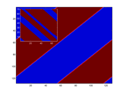
Figure 2: Microstructure obtained from the mean-field analysis of the Square-Rectangle (SR) spin model. The parameters are $L=128$, $\xi^{2}=0.5$, $E_{0}=3$, and $\tau=-2.5$, and stiffness $A_{1}=4$ with $2A_{1}/A_{3}=1$. Twins are oriented along a diagonal as expected. Inset: Twinned ground state from Monte Carlo simulations for the same parameters.

We now i) study effects of external uniform stress, ii) make contact with the phase diagram of the Blume-Capel model with uniform OP and iii) show how the Mean-field equations for $\sigma(\vec{r})$ can be obtained through the least-action principle.

III.1.1 Effects of external stress

Twins with oriented, locked-in domain walls of positive energy cost are metastable states, and the uniform single-variant state without domain walls is the global minimum in free energy. This can be seen by adding an external stress term $h(\vec{r})$ with a simple linear coupling to the meanfield hamiltonian (49):

$${\beta H_{ext}=-\dfrac{D_{0}}{2{\bar{\varepsilon}}(\tau)}\sum_{\vec{r}}h({\vec{r}})S({\vec{r}}}).$$ (57)

The meanfield self-consistency equations become

$${\sigma(\vec{r})=\dfrac{-2\sinh[V(\vec{r})-(D_{0}/2{\bar{\varepsilon}})h(\vec{r})]}{1+2\cosh[V(\vec{r})-(D_{0}/2{\bar{\varepsilon}})h(\vec{r})]}}.$$ (58)

Starting from random texture seeds with a small uniform external stress, $h=0.3$, we obtain a uniform state of $S=\pm 1$ depending on the sign of $h$: the small stress picks out the global minimum. The twins are self-trapped metastable states, that are however quite rigid against stress: for a twinned initial state, a strong stress of about $h=4$ needs to be applied to destroy the twins and to obtain the uniform ground state. Once the twins have vanished, the system fails to return to the original state, i.e. shows hysteretic behavior.

III.1.2 Blume-Capel model phase diagram

To make contact with treatments of the Blume-Capel model, we suppress the nonlocal couplings by setting $A_{1}=0$. The Ginzburg term in (6) can be recast on a lattice, by setting the gradient to a discrete difference operator $\vec{\nabla}\rightarrow\vec{\Delta}$, so that $({\vec{\nabla}}S)^{2}\rightarrow({\vec{\Delta}}S)^{2}=4S^{2}-2\sum_{<{\vec{r}}{\vec{r}}^{\prime}>}S(\vec{r})S(\vec{r}^{\prime})$. Then the hamiltonian is precisely a Blume- Capel model, bilinear in the spins (without the biquadratic term of the Blume-Emery-Griffiths model) R22 ,

$${H=-J(\tau)\sum_{<{\vec{r}}{\vec{r}}^{\prime}>}S(\vec{r})S(\vec{r}^{\prime})+\Delta(\tau)\sum_{\vec{r}}S(\vec{r})^{2}},$$ (59)

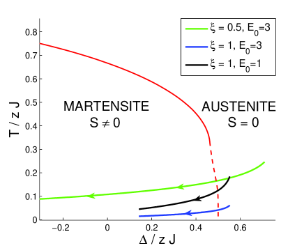
Figure 3: Mean-field phase diagram for the spin-1 model for the Square-Rectangle (SR) transition. The red solid line represents second-order phase transition and the red dashed line represents a first-order phase transition R22 , meeting at a tricritical point. The crystal field $\Delta(\tau)$ depends on the temperature $\tau$, so cooling is a phase-diagram trajectory. Three directed trajectories with different sets of parameters are shown, for cooling from $\tau=4/3$ to $\tau=-2.5$.The lines intersect the first-order transition line (dashed) for $\tau\simeq 1$.

There is temperature-dependence in the on-site crystal field term $\Delta(\tau)\equiv D_{0}(\tau)[g_{L}(\tau)+4\xi^{2}]/(2\beta)$, and in the ferromagnetic coupling $J(\tau)\equiv D_{0}(\tau)\xi^{2}/\beta$.

The model can be studied within the (uniform) mean-field approximation. An expansion of the mean-field free energy yields an analytical expression for the line of critical points $T_{c}=zJ/3$; and the location of the tricritical point, $\Delta_{c}=\frac{2}{3}zJ\log 2$, where $z=4$ is the number of nearest neighbors. Figure 3 shows the well-known phase diagram of this model. Both $\Delta$ and $J$ depend on the temperature $\tau$, so although a given temperature corresponds to a point, a cooling path is a line in the phase diagram. These lines intersect the first-order transition curve for $\tau\simeq 1$, the Landau transition temperature between ’ paramagnetic ’ austenite and ’ ferromagnetic ’ martensite. Figure 4 shows the meanfield phase diagram for two parameter planes $(h,\tau)$ and $(\xi,\tau)$. In a certain range of parameters, the spin model is consistent with the Landau theory that predicts a first-order phase transition at $\tau=1$.

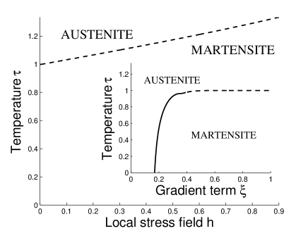
Figure 4: Mean-field phase diagram of the Square-Rectangle (SR) transition in the ($h$,$\tau$) plane for $\xi=1$. The $h=0$ first-order phase transition temperature of $\tau=1$ moves up with applied stress $h$. Inset: Phase diagram in the ($\xi$,$\tau$) plane. For $\xi$ large , there is a first-order phase transition line (dashed) with $\tau=1$, while for $\xi$ small, there is a second-order transition line (solid), that moves to lower temperature.

III.1.3 Field theory for $\sigma(\vec{r})$

We show here how the partition function may be transformed to obtain a field theory for $\sigma(\vec{r})=\langle S(\vec{r})\rangle$, so the mean-field equation (55) results from a saddle-point approximation of a functional integral. Other mean-field equations in this paper can similarly be obtained as saddle point approximations of field theories.

The partition function can be compactly written as

$${Z=\sum_{\left\{S\right\}}\exp\left(\frac{1}{2}\sum_{\vec{r}\vec{r}^{\prime}}S_{\vec{r}}K_{\vec{r}\vec{r}^{\prime}}S_{\vec{r}^{\prime}}\right)},$$ (60)

where $K_{\vec{r}\vec{r}^{\prime}}=\beta J(\tau)\delta_{<\vec{r},\vec{r}^{\prime}>}-\frac{D_{0}A_{1}}{2}U(\vec{r}-\vec{r}^{\prime})-2\beta\Delta(\tau)\delta_{\vec{r},\vec{r}^{\prime}}$. The first Kronecker symbol is non-zero only if $\vec{r}$ and $\vec{r}^{\prime}$ are neighbors. We note that the kernel $K_{\vec{r}\vec{r}^{\prime}}$ can be recast using usual matrix notations

$${K_{\vec{r}\vec{r}^{\prime}}=D_{0}\Braket{\vec{r}}{\xi^{2}\nabla^{2}-\frac{A_{1}}{2}U-g_{L}(\tau)}{\vec{r}^{\prime}}},$$ (61)

where $\langle\vec{r}|U|\vec{r}^{\prime}\rangle=U(\vec{r}-\vec{r}^{\prime})$. We may then use the standard Hubbard-Stratonovich transformation $\int e^{-\sum_{ij}A_{ij}x_{i}x_{j}+\sum_{i}B_{i}x_{i}}d^{n}x=\sqrt{\frac{\pi^{n}}{\det{A}}}e^{\frac{1}{4}B^{T}A^{-1}B}$ to find the exact integral representation of the partition function

$${Z=\frac{1}{(2\pi)^{N/2}\sqrt{\det K}}\int\prod_{\vec{r}}d\phi(\vec{r})\mathrm{e}^{-S[\phi]}},$$ (62)

with the action

$${S[\phi]=\frac{1}{2}\sum_{\vec{r}\vec{r}^{\prime}}\phi(\vec{r})K_{\vec{r}\vec{r}^{\prime}}^{-1}\phi(\vec{r}^{\prime})-\sum_{\vec{r}}\mathrm{log}\left(1+2\cosh(\phi(\vec{r}))\right)}.$$ (63)

Finally, we define $\sigma(\vec{r})=\sum_{\vec{r}^{\prime}}K^{-1}_{\vec{r}\vec{r}^{\prime}}\phi(\vec{r}^{\prime})$. The partition function reads

$${Z=\int\mathcal{D}[\sigma(\vec{r})]\mathrm{e}^{-S[\sigma]}},$$ (64)

where we have defined the formal measure $\mathcal{D}[\sigma(\vec{r})]=\sqrt{\det{K}}/(2\pi)^{N/2}\prod_{\vec{r}}d\sigma(\vec{r})$. With this field-theoretical formulation of the partition function, our problem, the Mean-field approximation is obtained by minimizing the action

$$\displaystyle S[\sigma] =\frac{1}{2}\sum_{\vec{r}\vec{r}^{\prime}}\sigma(\vec{r})K_{\vec{r}\vec{r}^{\prime}}\sigma(\vec{r}^{\prime})$$ (65)

$$-\sum_{\vec{r}}\mathrm{log}\left(1+2\cosh(\sum_{\vec{r}^{\prime}}K_{\vec{r}\vec{r}^{\prime}}\sigma(\vec{r}^{\prime}))\right).$$

Within the saddle-point approximation, $\sigma(\vec{r})=\langle S(\vec{r})\rangle$ so that the field $\sigma$ is indeed the statistical average of the spin. We note that $V(\vec{r})=-\sum_{\vec{r}^{\prime}}K_{\vec{r}\vec{r}^{\prime}}\sigma(\vec{r}^{\prime})$ (eq. (52)), so the minimization of the action yields the mean-field equation (55), as expected.

III.2 Triangle/Centred-Rectangle (TCR) meanfield: $N_{OP}=1,N_{V}=3$

The TCR case spin hamiltonian is (38), with spin values $\vec{S}=(0,0),(1,0)(-1/2,\pm\sqrt{3}/2)$ of (36) and $g_{L}$ as in (37). Since $N_{OP}=2$ for the TCR, SO, TO and CT transitions, their meanfield equations are all formally the same. From the substitution $\vec{S_{\ell}}(\vec{r})=\vec{\sigma_{\ell}}(\vec{r})+\delta\vec{S}(\vec{r})$ and linearization in $\delta\vec{S}(\vec{r})\equiv\vec{S_{\ell}}(\vec{r})-\vec{\sigma_{\ell}}(\vec{r})$ the meanfield hamiltonian is $\beta H_{MF}\equiv\sum_{\vec{r}}\beta h_{MF}(\vec{r})-C$, as in (49) but the local contribution is now

$${\sum_{\vec{r}}\beta h_{MF}(\vec{r})=\sum_{{\vec{r}},\ell=2,3}V_{\ell}(\vec{r})S_{\ell}(\vec{r})=\sum_{{\vec{k}},\ell}V_{\ell}(\vec{k})S_{\ell}(\vec{k})^{*}}$$ (66)

and $C\equiv\frac{1}{2}\sum\langle\beta h_{MF}\rangle=\frac{1}{2}\sum_{\vec{k},\ell}V_{\ell}(\vec{k})\sigma_{\ell}(\vec{k})^{*}$. The functions $V_{2}$ and $V_{3}$ are defined in Fourier space by

$${V_{2}(\vec{k})=P_{2}^{0}(\vec{k})\sigma_{2}(\vec{k})+\frac{D_{0}A_{1}}{2}U_{23}(\vec{k})\sigma_{3}(\vec{k})},$$ (67)

$${V_{3}(\vec{k})=P_{3}^{0}(\vec{k})\sigma_{3}(\vec{k})+\frac{D_{0}A_{1}}{2}U_{32}(\vec{k})\sigma_{2}(\vec{k})}.$$ (68)

where

$${P_{\ell}^{0}(\vec{k})=D_{0}[g_{L}+\xi^{2}\vec{k}^{2}+\frac{A_{1}}{2}U_{\ell\ell}(\vec{k})]}.$$ (69)

Defining $P_{\ell}$ in Fourier space as $P_{\ell}(\vec{k})\equiv P_{\ell}^{0}(\vec{k})\sigma_{\ell}(\vec{k})$, the coordinate space meanfield hamiltonian of (III.2) is then

$$\displaystyle\beta h_{MF}(\vec{r}) =\sum_{\ell}P_{\ell}(\vec{r})S_{\ell}(\vec{r})$$ (70)

$$+\dfrac{D_{0}A_{1}}{2}\sum_{\vec{r}^{\prime}}U_{23}(\vec{r}-\vec{r}^{\prime})[\sigma_{2}(\vec{r})S_{3}(\vec{r}^{\prime})+\sigma_{3}(\vec{r}^{\prime})S_{2}(\vec{r}))].$$

The partition function of this linearized meanfield Hamiltonian can again be factorized as in (53).

The self-consistency equations as in (53), (54) for the statistical averages $\left\{\vec{\sigma}(\vec{r})\right\}$ again have the constant $C$ cancelling, so now with $\vec{V}=(V_{2},V_{3})$ and $\vec{S}=(S_{2},S_{3})$,

$${\vec{\sigma}(\vec{r})=\sum_{\vec{S}(\vec{r})}~{}\vec{S}(\vec{r})\mathrm{e}^{-{\vec{V}}(\vec{r}).{\vec{S}}(\vec{r})}/\sum_{\vec{S}(\vec{r})}\mathrm{e}^{-{\vec{V}}(\vec{r}).{\vec{S}}(\vec{r})}}.$$ (71)

In terms of the $N_{V}$ variant states $\vec{S}=(\cos\phi_{m},\sin\phi_{m})$ with $m=1,2...N_{V}$ this can be formally expressed for TCR, SO, TO and CT cases as

$${\sigma_{2}=\dfrac{\sum_{m=1}^{N_{V}}\cos\phi_{m}\mathrm{e}^{-(\cos\phi_{m}V_{2}+\sin\phi_{m}V_{3})}}{1+\sum_{m=1}^{N_{V}}\mathrm{e}^{-(\cos\phi_{m}V_{2}+\sin\phi_{m}V_{3})}}},$$ (72)

$${\sigma_{3}=\dfrac{\sum_{m=1}^{N_{V}}\sin\phi_{m}\mathrm{e}^{-(\cos\phi_{m}V_{2}+\sin\phi_{m}V_{3})}}{1+\sum_{m=1}^{N_{V}}\mathrm{e}^{-(\cos\phi_{m}V_{2}+\sin\phi_{m}V_{3})}}}.$$ (73)

For the TCR case sums over the $N_{V}=3$ spin values of (36), this is

$${\sigma_{2}=\dfrac{1}{2}\dfrac{\textrm{e}^{-\frac{3}{2}V_{2}}-\cosh(\frac{\sqrt{3}}{2}V_{3})}{[\textrm{e}^{-V_{2}}\cosh(\frac{V_{2}}{2})+\cosh(\frac{\sqrt{3}}{2}V_{3})]}},$$ (74)

$${\sigma_{3}=-\dfrac{\sqrt{3}}{2}\dfrac{\sinh(\frac{\sqrt{3}}{2}V_{3})}{[\textrm{e}^{-V_{2}}\cosh(\frac{V_{2}}{2})+\cosh(\frac{\sqrt{3}}{2}V_{3})]}}.$$ (75)

where the position dependences of $\sigma_{\ell}(\vec{r})$ and $V_{\ell}(\vec{r})$ are left implicit. The coupled equations (74), (75) were solved iteratively on a $L\times L=256\times 256$ lattice with periodic boundary conditions with parameter values $\xi^{2}=0.8$, $A_{1}=5$, $\tau=-6.5$, and $E_{0}=0.01$. Here, and throughout the following other cases, $T_{0}=1.0$, $T_{c}=0.9$.

Figure 5 shows the relaxed microstructure obtained after $10^{5}$ iteration steps. As in continuous-variable simulations in strains or displacements R4 ; R7 we also obtain nested-star patterns as observed in experiments R8 for lead orthovanadate. However, unlike the continuous-variable models which are computationally intensive, the spin models and the local meanfield solutions reach the complex microstructure relatively rapidly.

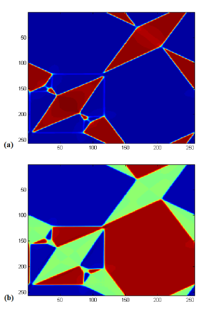
Figure 5: Final-state microstructure obtained from meanfield self-consistency equations for the Triangle-Centred Rectangle (TCR) transition: (a) strain component $e_{2}$ ; (b) strain component $e_{3}$. The color code of red (blue) corresponds to positive (negative) values, and green to zero. Note the sharp domain walls. Parameters are $L=256$, $\xi^{2}=0.8$, $E_{0}=0.01$, scaled temperature $\tau=-6.5$ and stiffness $A_{1}=5$.

III.3 Square/Oblique (SO) meanfield: $N_{OP}=2,N_{V}=4$

The SO case spin Hamiltonian is formally the same as (38) but with SO case spin values $\vec{S}=(\pm 1/\sqrt{2},\pm 1/{2})$ of (43), and $g_{L}$ is as in (44). Doing a local meanfield approximation as before, the formal self-consistency equations of  (72),  (73) become

$${\sigma_{2}=-\dfrac{1}{\sqrt{2}}\dfrac{2\sinh(\frac{V_{2}+V_{3}}{\sqrt{2}})+2\sinh(\frac{V_{2}-V_{3}}{\sqrt{2}})}{[1+2\cosh(\frac{V_{2}+V_{3}}{\sqrt{2}})+2\cosh(\frac{V_{2}-V_{3}}{\sqrt{2}})]}},$$ (76)

$${\sigma_{3}=-\dfrac{1}{\sqrt{2}}\dfrac{2\sinh(\frac{V_{2}+V_{3}}{\sqrt{2}})-2\sinh(\frac{V_{2}-V_{3}}{\sqrt{2}})}{[1+2\cosh(\frac{V_{2}+V_{3}}{\sqrt{2}})+2\cosh(\frac{V_{2}-V_{3}}{\sqrt{2}})]}}.$$ (77)

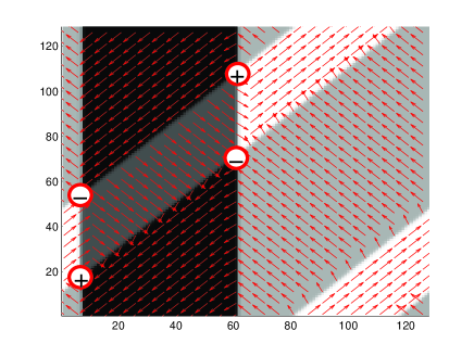
Figure 6: Final state microstructure from meanfield equations for the Square-Oblique (SO). The four variants are in four different colors, and pseudospin spins orientations are also denoted. The discretized vortices (topological charge $+1$) and anti-vortices (topological charge $-1$), expected in the classical clock models, are also identified. Parameters used are $L=128$, $\xi^{2}=0.3$, $E_{0}=0.2$, and $\tau=-2.5$ and $A_{1}=6$.

The coupled equations were solved iteratively on a $128\times 128$ lattice with periodic boundary conditions and for different temperatures $\tau$, starting from an initial random texture. Figure 6 shows that the microstructure obtained for $\tau=-2.5$, has vortices, as in the classical clock models or in the XY model. This vortex in the strain field differs of course, from an edge dislocation that is a structural defect in the displacement field. The pseudospin vortex at the meeting point of domain walls is characterized by the winding number or topological charge

$${q_{i}=\frac{1}{2\pi}\oint_{\Gamma_{i}}\vec{\nabla}\theta.d\vec{r}},$$ (78)

where $\theta(\vec{r})$ is the polar angle of the spin $\vec{S}(\vec{r})$, that equals $\phi_{m}$ in the variant regions, and $\Gamma_{i}$ is an arbitrary contour surrounding the $i$-th vortex. The topological charge is $q_{i}=1$ for a vortex and $q_{i}=-1$ for an anti-vortex. Thanks to the periodic boundary conditions, we have $\sum_{i}q_{i}=0$. Vortex solutions for complex fields at three-domain meeting points have been considered R23 .

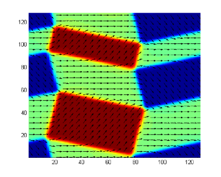
Figure 7: Final state microstructure from meanfield equations for the Triangle-Oblique (TO). The three variants are in three different colors, and spin orientations are also shown. Only three of the six variants (see Fig 8), finally survive. Parameters used are $L=128$, $\xi^{2}=0.35$, $E_{0}=0.2$, scaled temperature $\tau=-2.6$, and stiffness $A_{1}=5$.

III.4 Triangle/Oblique (TO) meanfield: $N_{OP}=2,N_{V}=6$

The TO case hamiltonian is as in (38) but with TO case spin values $\vec{S}=(0,0),(\pm 1,0),(\pm 1/2,\pm\sqrt{3}/2)$ from  (47), and $g_{L}$ is as in (48). The general meanfield self-consistency equations of (72),  (73) are then

$${\sigma_{2}=-\dfrac{2\sinh(V_{2})+\sinh(I)+\sinh(J)}{1+2\cosh(V_{2})+2\cosh(I)+2\cosh(J)}},$$ (79)

$${\sigma_{3}=-\frac{\sqrt{3}}{2}\dfrac{2\sinh(I)-2\sinh(J)}{1+2\cosh(V_{2})+2\cosh(I)+2\cosh(J)}},$$ (80)

where $I=(V_{2}+\sqrt{3}V_{3})/2$ and $J=(V_{2}-\sqrt{3}V_{3})/2$. Figure 7 shows the ground state obtained from these coupled meanfield equations with parameters $L=128$, $\xi^{2}=0.35$, $E_{0}=0.2$, $\tau=-2.6$ and $A_{1}=5$. We note that discrete vortices at the junction of the six martensite variants, are seen only during the iterations through transient states as in Figure 8. The final state microstructure shows no vortices, and only three out of the six variants finally remain, bounded by nonintersecting domain walls, as the other variants vanish during the course of the textural evolution. The suppression of vortices at least for these parameter values, could be due to the energy costs of the gradient and powerlaw terms.

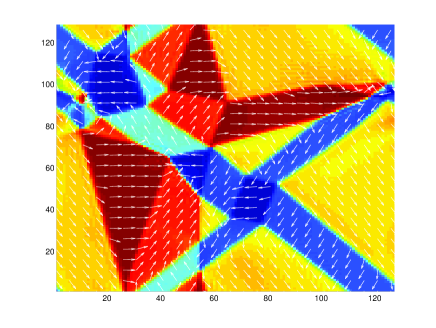
Figure 8: Transient state for the (TO) transition with the six variants with different colors, with parameters as for Fig 7.

IV PSEUDOSPIN HAMILTONIAN AND LOCAL MEANFIELD IN THREE SPATIAL DIMENSIONS

We outline the hamiltonian derivations for the cubic/tetragonal case and then do a meanfield analysis. The approach can also be followed for other 3D transitions R17 .

IV.1 Cubic/Tetragonal (CT) hamiltonian: $N_{OP}=2,N_{V}=3$

For the cubic-to-tetragonal or ’CT’ transition, the symmetry-adapted strains are the dilatation $e_{1}=(1/\sqrt{3})(e_{xx}+e_{yy}+e_{zz})$, the two deviatoric OP strains $e_{2}=(1/\sqrt{2})(e_{xx}-e_{yy})$, $e_{3}=(1/\sqrt{6})(e_{xx}+e_{yy}-2e_{zz})$, and the three shear strains $e_{4}=2e_{yz}$, $e_{5}=2e_{zx}$, $e_{6}=2e_{xy}$.

The OP components are the two deviatoric strains $\vec{e}=(e_{3},e_{2})$, and the remaining four non-OP compressional and shear strains are $e_{1},e_{4},e_{5},e_{6}$. The Landau free energy invariant under symmetries of the cubic unit-cell, was originally given by Barsch and Krumhansl R10 , where the cubic invariant is now $I_{3}=(e_{3}^{3}-3e_{3}e_{2}^{2})$, and in scaled form is

$$f_{L}=\tau(e_{2}^{2}+e_{3}^{2})-2(e_{3}^{3}-3e_{3}e_{2}^{2})+(e_{2}^{2}+e_{3}^{2})^{2}.$$ (81)

The Ginzburg term is formally identical to (29) but in 3D.

The non-OP terms, harmonic in the four remaining physical strains are

$${f_{non}=\frac{A_{1}}{2}e_{1}^{2}+\frac{A_{4}}{2}(e_{4}^{2}+e_{5}^{2}+e_{6}^{2})}.$$ (82)

and are minimized subject to the compatibility constraint (8) in 3D. There are six equations, from cyclic permutations of the labels $x,y,z$ of the two equations

$${2\partial_{x}\partial_{y}e_{yz}-\partial^{2}_{z}e_{yy}-\partial^{2}_{y}e_{zz}=0},$$ (83)

$${\partial_{y}\partial_{z}e_{xx}+\partial^{2}_{x}e_{yz}-\partial_{x}\partial_{y}e_{zx}-\partial_{x}\partial_{z}e_{xy}=0}.$$ (84)

By going to Fourier space one finds the second set is an identity, if the first set is satisfied. These constraint equations can be recast in terms of the symmetry-adapted strains $e_{1},e_{2}...e_{6}$. Minimizing ${\bar{F}}_{non}$ with these constraints (either through Lagrange multipliers R7 , or through direct solution for $e_{4},e_{5},e_{6}$ and minimization R17 in the remaining $e_{1}$), yields the non-OP strains in terms of the OP strains $e_{2}$ and $e_{3}$. Substitution into the harmonic non-OP free energy yields the compatibility term

$${{\bar{F}}_{compat}=\frac{1}{2}\sum_{\ell,\ell^{\prime}=2,3}\sum_{\vec{k}}A_{1}U_{\ell\ell^{\prime}}(\vec{k})e_{\ell}(\vec{k})e_{\ell^{\prime}}(\vec{k})^{*}},$$ (85)

where the kernels $U_{\ell,\ell^{\prime}}(\vec{k})$ in Fourier space R17 are given in the Appendix.

The procedure is formally just as in the TCR case, as the CT case also has the same $N_{OP}=2,N_{V}=3$, pseudo-spin values $\vec{S}=(0,0),(1,0),(-1/2,\pm\sqrt{3}/2)$ and again $\bar{\varepsilon}(\tau)=3/4(1+\sqrt{1-8\tau/9})$. The spatial dimension only enters in the 3D compatibility potential of kernels (85), and in the 3D lattice positions $\vec{r}=(x,y,z)$ and Brillouin zone wave-vectors $\vec{k}=(k_{x},k_{y},k_{z})$.

IV.2 Cubic/Tetragonal meanfield : $N_{OP}=2,N_{V}=3$

We numerically solved the CT meanfield equations (74), (75) that are as for the TCR case, with the kernels as in the Appendix. We took a $32\times 32\times 32$ lattice with periodic boundary conditions, and parameters $\xi^{2}=10$, $E_{0}=0.001$, $T_{0}=1,T_{c}=0.9$, and stiffnesses $A_{1}=4.8$, $A_{4}=2.4$. Fourier transforms enable a computation at each step, of the functions $V_{2}(\vec{r})$ and $V_{3}(\vec{r})$. Figure 9 shows the microstructure, with twins at diagonal orientations, as found in continuous-variable simulations.

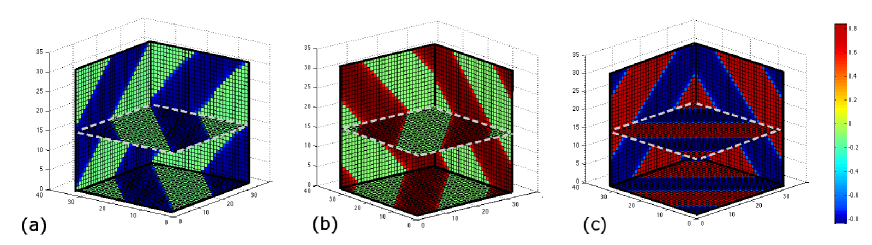
Figure 9: Twins in the (111) plane obtained from the meanfield self-consistency equations for the 3D cubic-to-tetragonal transformation. The color bar represents $S_{y}$. The parameters are $L=32$, $\xi^{2}=10$, $E_{0}=0.001$, scaled temperature $\tau=-0.5$ and stiffnesses $A_{1}=4.8$, $A_{4}=2.4$. The microstructures (a),(b), and (c) show three different twin orientations obtained, for different runs.

V OTHER RELATED MODELS

Modified truncations of these structural-transition free energies can induce other hamiltonians, that can be studied purely as interesting spin models in statistical mechanics.

Let us suppress the zero state, and fix only the circle radius $\varepsilon\rightarrow{\bar{\varepsilon}}(\tau)$, while keeping all continuous polar angles, now denoted by $\theta(\vec{r})$, with values $2\pi>\theta\geq 0$,

$$\vec{e}(\vec{r})=\begin{pmatrix}e_{2}(\vec{r})\\ e_{3}(\vec{r})\end{pmatrix}\rightarrow{\bar{\varepsilon}}(\tau)\begin{pmatrix}\cos\theta(\vec{r})\\ \sin\theta(\vec{r})\end{pmatrix}$$ (86)

so as in the XY model of planar spins, ${\vec{S}}=(\cos\theta,\sin\theta)$. The Ginzburg discrete-difference term of (6) then induces an XY- like ferromagnetic interaction. The Landau free energy in polar coordinates in all cases has angular dependence ${\bar{f}}_{L}\sim-B\cos N_{V}\phi$ as in  (27),  (42),  (46). Putting all this together, the free energy induces an XY ferromagnet model with a long-range potential, and a symmetry-breaking local field :

$$\displaystyle\beta H =\frac{D_{0}}{2}[-B\sum_{\vec{r}}\cos[N_{V}\theta(\vec{r})]$$

$$-2\xi^{2}\sum_{<\vec{r},\vec{r}^{\prime}>}\cos(\theta(\vec{r})-\theta(\vec{r}^{\prime}))]+\beta H_{C}(\{\theta\})$$ (87)

Here as ${\vec{S}}^{2}=1$, there is no quadratic local term, and $\beta H_{C}(\{\theta\})$ is a term coupling the continuous-angle variables $\cos\theta(\vec{r})$ and $\sin\theta(\vec{r})$,

$$\displaystyle\beta H_{C}[\{\theta\}] =\frac{A_{1}D_{0}}{4}\sum_{{\vec{r}},{\vec{r}}^{\prime}}U_{22}\cos\theta(\vec{r})\cos\theta(\vec{r}^{\prime})$$

$$+U_{33}\sin\theta(\vec{r})\sin\theta(\vec{r}^{\prime})$$

$$+U_{23}\cos\theta(\vec{r})\sin\theta(\vec{r}^{\prime})+U_{32}\sin\theta(\vec{r})\cos\theta(\vec{r}^{\prime})$$ (88)

and a partition function

$${Z=\int_{[0,2\pi]^{N}}\prod_{\vec{r}}d\theta(\vec{r})\exp(-\beta H[\{\theta(\vec{r})\};\tau])}.$$ (89)

This model includes all angles, even away from minima, and so can describe slowly transiting states across $N_{V}$ saddle points, as in experiment R24 .

Similar XY models with symmetry-breaking fields (without the powerlaw interaction) have been studied R24 . A dual transform in that case extracts the topological vortices with logarithmic interactions, and in this model could also induce a powerlaw anisotropic vortex interaction. A real-space renormalization group analysis of the 2D Coulomb gas as in the Kosterlitz -Thouless transition is well-known R25 , and could be repeated for this model. Renormalization flows in the context of martensitic transitions have been studied in other models R26 .

For strong symmetry-breaking in minima angular directions ( $|B|$ large), the continuous angle $\theta$ become discrete and takes on values that we denote as $\theta\rightarrow\phi=\phi_{m}$, and one gets pure clock models ($\mathbb{Z}_{N_{V}}$) with a Hamiltonian that now has powerlaw potentials,

$${\beta H_{clock}=-D_{0}\xi^{2}\sum_{<{\vec{r}}{\vec{r}^{\prime}}>}\cos[\phi(\vec{r})-\phi(\vec{r}^{\prime})]+\beta H_{C}(\{\phi\})}.$$ (90)

We can even make one more approximation by reducing the XY interaction to a Kronecker-delta coupling, yielding a $q$-state Potts R19 model with $q=N_{V}$:

$${\beta H_{Potts}=-D_{0}\xi^{2}\sum_{<{\vec{r}}{\vec{r}^{\prime}}>}\delta_{\vec{S}(\vec{r}),\vec{S}(\vec{r}^{\prime})}+\beta H_{C}(\{\phi\})}.$$ (91)

Potts hamiltonians with large number of spin components $q$ have been studied as models for configurational glasses R19 .

VI Conclusion

A standard approach to obtaining microstructure of structural transitions is to solve evolution equations for relaxation to a minimum, in continuous variables such as displacements, phase fields or strains R4 ; R5 ; R6 ; R7 . We have here considered the reduced hamiltonian models in discrete pseudospins describing four structural transitions in two dimensions, as well as the three dimensional cubic-to-tetragonal transition. These ’clock-zero’ models have a zero state as well as clock states, and the pseudospin hamiltonian has an on-site term, an exchange interaction and a powerlaw interaction term. For the square/rectangle case, the pseudo-spin model without powerlaw interactions corresponds to the Blume-Capel spin-1 model with temperature-dependent couplings. Using a local meanfield approach, we have obtained the microstructure for 2D and 3D transitions, as obtained in continuous-variable strain dynamics. For example, the characteristic nested star microstructure of the triangle transition emerges easily from the meanfield solution.

The textures of the square/oblique (SO) and triangle/oblique (TO) transitions, with $N_{V}=4,6$, which have not been previously studied, include vortex configurations of the $\mathbb{Z}_{N_{V}+1}$ clock models, at intersections between variant domain walls. The SO final microstructure has positive/negative vortices in regular patterns, and all four variants are present. For the TO case, at least for particular parameters, we find the six-variant-vortices appear only as transient solutions, with the final state having no vortices, with only non-intersecting closed-domains of three variants. Finally, for the three dimensional cubic/tetragonal transition, we obtain the diagonal twinning that is consistent with previous studies R4 ; R6 ; R7 . In all cases, the local meanfield final microstructure emerges relatively rapidly, compared to the slow evolution towards steady-state of the continuum differential-equation dynamics.

Further work can involve studies of pseudospin hamiltonians R17 for other structural transitions in 2D and 3D in the local meanfield approach. By including quenched disorder, such pseudo-spin models may be used to study strain glass behavior in martensitic alloys R21 , and relate solutions to the tweed precursors R5 in analogy with spin-glass like behavior, and to random-field models R16 . Monte Carlo simulations can be used to study martensitic nucleation and growth R27 . Other related spin models of interest in their own right may include geometric nonlinearities that yield complex heirarchical-twin patterns R2 ; R4 .

In conclusion, the discrete-variable pseudospin model in local meanfield approximation, is therefore a useful approach to the study of martensitic texturing.

Appendix A Kernels for the cubic-to-tetragonal transition

In this Appendix we state the explicit form of the bulk kernels $U_{\ell\ell^{\prime}}$ obtained elsewhere R17 for the 3D cubic-to-tetragonal transition. To do so we define the coefficients $O^{(s)}_{\alpha}$ and $O_{\alpha}$ by

$${O_{1}^{(4)}=\frac{-1}{\sqrt{3}}(k_{y}^{2}+k_{z}^{2}),O_{2}^{(4)}=\frac{k_{z}^{2}}{\sqrt{2}},O_{3}^{(4)}=\frac{1}{\sqrt{6}}(2k_{y}^{2}-k_{z}^{2})},$$ (92)

$${O_{1}^{(5)}=\frac{-1}{\sqrt{3}}(k_{x}^{2}+k_{z}^{2}),O_{2}^{(5)}=\frac{-k_{z}^{2}}{\sqrt{2}},O_{3}^{(5)}=\frac{1}{\sqrt{6}}(2k_{x}^{2}-k_{z}^{2})},$$ (93)

$${O_{1}^{(6)}=\frac{-1}{\sqrt{3}}(k_{y}^{2}+k_{x}^{2}),O_{2}^{(6)}=\frac{1}{\sqrt{2}}(k_{x}^{2}-k_{y}^{2}),O_{3}^{(6)}=\frac{-1}{\sqrt{6}}(k_{x}^{2}+k_{y}^{2})},$$ (94)

$${O_{4}=k_{y}k_{z},O_{5}=k_{x}k_{z},O_{6}=k_{x}k_{y}},$$ (95)

Let $\bar{O}^{(s)}_{\alpha}=O^{(s)}_{\alpha}/O_{s}$ and $G_{\alpha\beta}=\sum_{s}(A_{s}/A_{1})\bar{O}^{(s)}_{\alpha}\bar{O}^{(s)}_{\beta}$. The compatibility kernel for the cubic/tetragonal transition can then be written as the $2\times 2$ matrix

$${U_{\ell,\ell^{\prime}}=\nu(\vec{k})\dfrac{G_{\ell\ell^{\prime}}+\{G_{\ell\ell^{\prime}}G_{11}-G_{\ell 1}G_{\ell^{\prime}1}\}}{1+G_{11}}}.$$ (96)

where $\nu(\vec{k})\equiv(1-\delta_{{\vec{k}},0})$ sets the non-OP harmonic-energy contribution for uniform strains to its minimum value of zero.