On non-local representations of the ageing algebra

Malte Henkel^a and Stoimen Stoimenov^b

^a Groupe de Physique Statistique, Département de Physique de la Matière et des Matériaux,

Institut Jean Lamour,Nancy Université (UMR 7198 – CNRS – UHP – INPL – UPVM)

B.P. 70239, F – 54506 Vandœuvre lès Nancy Cedex, France

^b Institute of Nuclear Research and Nuclear Energy, Bulgarian Academy of Sciences,

72 Tsarigradsko chaussee, Blvd., BG – 1784 Sofia, Bulgaria

The ageing algebra is a local dynamical symmetry of many ageing systems, far from equilibrium, and with a dynamical exponent $z=2$. Here, new representations for an integer dynamical exponent $z=n$ are constructed, which act non-locally on the physical scaling operators. The new mathematical mechanism which makes the infinitesimal generators of the ageing algebra dynamical symmetries, is explicitly discussed for a $n$-dependent family of linear equations of motion for the order-parameter. Finite transformations are derived through the exponentiation of the infinitesimal generators and it is proposed to interpret them in terms of the transformation of distributions of spatio-temporal coordinates. The two-point functions which transform co-variantly under the new representations are computed, which quite distinct forms for $n$ even and $n$ odd. Depending on the sign of the dimensionful mass parameter, the two-point scaling functions either decay monotonously or in an oscillatory way towards zero.

1 Introduction

Non-relativistic space-time transformations have recently met with a lot of interest – in addition to fields such as hydrodynamics [43, 52], they have been playing an increasing rôle in the analysis of the long-time behaviour of strongly interacting many-body systems far from equilibrium [12, 27] and even more recently have arisen in non-relativistic limits of the AdS/CFT correspondence, see e.g. [4, 38, 3, 32], with interesting applications to cold atoms [47, 15]. One of the ingredients for physically interesting sets of space-time transformations appears to be some kind of conformal invariance and recently, a classification of non-relativistic conformal space-time transformations was presented [14]. An important sub-set of these is characterised by a finite dynamical exponent $0<z<\infty$. Indeed, the list of sets of admissible generators which close into a Lie algebra is a rather short one, in $d+1$ space-time dimensions:

1. the conformal algebra itself, in $d+1$ dimensions, with $z=1$.

2. the Schrödinger algebra, which was discovered by Lie in 1881 as a dynamical symmetry algebra of the $1D$ free diffusion equation. The dynamical exponent is $z=2$. This algebra was rediscovered in physics as a symmetry of free non-relativistic particles several times around 1970, including [33, 18, 40, 31]. Non-linear examples of Schrödinger-invariant equations include the Navier-Stokes equation [43, 19, 42] or Burger’s equation [41, 30], see e.g. [27] and refs. therein for a short summary of further examples. Schrödinger symmetry (or rather its sub-algebra with time-translations left out) also arises in the far-from-equilibrium dynamics of statistical systems [21], for example in simple magnets quenched to a temperature $T<T_{c}$ below the critical temperature $T_{c}>0$ from a fully disordered initial state when $z=2$ is known [9, 12, 27].

3. the conformal galilean algebra cga$(d)$ appears to have been first identified in [20], but was independently rediscovered in different contexts [22, 39]. It is usually obtained, by a contraction, as the non-relativistic limit of the $(d+2)$-dimensional conformal algebra (itself obtained by a non-relativistic holographic construction) [24, 37, 1, 2, 34, 35, 32]. In $d=1$ space dimension, there exists an infinite-dimensional extension which can be constructed from a contraction of a pair of commuting Virasoro algebras [23, 26, 2]. In most representations, one has $z=1$, but representations with $z=2$ are also known [26].

4. in $d=2$ space dimensions, there exists the exotic conformal galilean algebra ecga, which is the central extension of the non-semi-simple cga$(2)$ [36]. Although one may readily identify linear equations invariant under ecga [37], the construction of invariant non-linear equations is not straightforward [52, 11]. The dynamical exponent is $z=1$. See [29] for a recent review and the relationship with non-commutative mechanics.

5. finally, there exists for $d=1$ a closed algebra with $z=\frac{3}{2}$ [23]. It is not yet clear how this might fit into the general scheme of [14], since it does not contain the full conformal structure and furthermore its generators contain fractional space derivatives.

This short list illustrates the practical difficulty of constructing sets of ‘conformal’ space-time transformations for a generic dynamical exponent $z\neq 1,2$ such that a Lie algebra is obtained. It is at present not fully understood how to construct a dynamical symmetry even for a simple linear equation of the form (where $z\neq 1,2$)

$${\cal S}\psi(t,r):=\bigl{(}z\mu\partial_{t}-\partial_{r}^{z}\bigr{)}\psi(t,r)=0$$ (1.1)

which arises as one of the most simple equations of motion of the order-parameter in studies of ageing far from equilibrium [10, 8]. Indeed, current attempts to find further dynamical symmetries of eq. (1.1) beyond the obvious translation-, dilatation- and rotation-symmetries (if $d>1$) only succeed at the price that the further generators must be required to vanish on certain states (which are then declared to be the ‘physical’ ones) [22, 23, 27]. Furthermore, these generators cannot, in general, be expressed in terms of first-order differential operators (‘vector fields’ in mathematical terminology). In the context of statistical physics, the order- parameter does not really satisfy a deterministic equation, but rather the r.h.s of (1.1) is replaced by a random noise term, which leads to a Langevin equation. However, since the non-relativistic algebras mentioned above are all non-semi-simple and their representations are projective, it is possible to study first the symmetries of the deterministic equation (1.1) and then use the resulting Bargman super-selection rules [5] in order to reduce the calculation of any average to the calculation of averages within the deterministic part of the theory as defined by (1.1) [44]. This procedure works not only for thermal noises and a simple diffusion equation with $z=2$, but can be generalised to generic values of $z$ and fairly general noises, such as they may arise in reaction-diffusion systems [6, 45, 7, 8, 13], see [27] for a systematic presentation.

In this paper, we shall explore properties of a new kind of representations of the common sub-algebra $\mathfrak{age}(d)$ of the Schrödinger and conformal galilean algebras. For the sake of notational simplicity, we shall restrict from now on to $d=1$ spatial dimensions. Then the standard representation, on sufficiently differentiable space-time functions $f(t,r)$, of the Lie algebra $\mathfrak{age}(1):=\bigl{\langle}X_{0,1},Y_{\pm\frac{1}{2}},M_{0}\bigr{\rangle}$ is given by

$$X_{0} = -t\partial_{t}-\frac{1}{2}r\partial_{r}-\frac{x}{2}\hskip 89.626pt\mbox{\rm dilatation}$$

$$X_{1} = -t^{2}\partial_{t}-tr\partial_{r}-\frac{\cal M}{2}r^{2}-(x+\xi)t\hskip 14.22636pt\mbox{\rm special transformation}$$

$$Y_{-\frac{1}{2}} = -\partial_{r}\hskip 154.21388pt\mbox{\rm space-translations}$$ (1.2)

$$Y_{\frac{1}{2}} = -t\partial_{r}-{\cal M}r\hskip 114.38019pt\mbox{\rm Galilei-transformation}$$

$$M_{0} = -{\cal M}\hskip 149.94614pt\mbox{\rm phase shift}$$

See (2.2) for the commutators. This representation is characterised by the ‘mass’ $\cal M$ and the pair of scaling dimensions $(x,\xi)$ whose values depend on the scaling operator on which these generators act. If one defines the Schrödinger operator

$${\cal S}:=2{\cal M}\partial_{t}-\partial_{r}^{2}+2{\cal M}\left(x+\xi-\frac{1}{2}\right)\frac{1}{t}$$ (1.3)

then the equation ${\cal S}\psi(t,r)=0$ has $\mathfrak{age}(1)$ as dynamical symmetry, because of the commutation relations

$$\bigl{[}{\cal S},Y_{\pm\frac{1}{2}}\big{]}\>=\>\bigl{[}{\cal S},M_{0}\bigr{]}\>=\>0\;\;,\;\;\bigl{[}{\cal S},X_{0}\bigr{]}\>=\>-{\cal S}\;\;,\;\;\bigl{[}{\cal S},X_{1}\bigr{]}=-2t{\cal S}$$ (1.4)

which imply that any solution of ${\cal S}\psi=0$ is mapped onto another solution of the same equation. A physical example for (1.3) is given by the relaxation kinetics of the spherical model, or equivalently the $N\to\infty$ limit of the O($N$) model, after a quench to a temperature $T\leq T_{c}$ at or below its critical temperature $T_{c}>0$ [16]. The representation (1.2) has a dynamical exponent $z=2$ and acts locally on the space-time coordinates. We point out that because time-translations (with a generator $X_{-1}=-\partial_{t}$) are not included and hence a system with an $\mathfrak{age}$-symmetry is not at a stationary state, the scaling dimension $\xi$ arises as a further universal characteristics of the relaxation process. By the transformation $\phi(t,r)=t^{\xi_{\phi}}\Phi(t,r)$, the physical $\mathfrak{age}$-quasi-primary field $\phi$ with scaling dimensions $(x_{\phi},\xi_{\phi})$ can be related to the Schrödinger-quasi-primary field $\Phi$ with scaling dimensions $(x_{\Phi}=x_{\phi}+2\xi_{\phi},\xi_{\Phi}=0)$ [25] and in the transformed eq. (1.3) $x+\xi$ is replaced by $x_{\Phi}$. If this option is chosen, one must give up the identity of physical and quasi-primary scaling operators, familiar from conformal invariance, which holds for stationary, equilibrium systems. The potential term in (1.3) can of course be eliminated by a similar transformation or else by imposing the constraint $x+\xi=\frac{1}{2}$.

When trying to extend (1.2) to a representation of cga$(1)\supset\mathfrak{age}(1)$, the extra generators are not necessarily first-order differential operators [24]. We believe that this fact should be taken seriously and its consequences studied. For this reason, and in order to find further representations of $\mathfrak{age}(1)$ with different values of $z$, we shall give in section 2 non-local representations of $\mathfrak{age}(1)$, which admit any integer value $z=n\in\mathbb{N}$, but which cannot be reduced to first-order differential operators. As we shall see, closure of these representations requires to restrict the representation space by performing a quotient with respect to the Schrödinger equation ${\cal S}\psi=0$. In section 3, we address the question how to interpret geometrically such infinitesimal generators by explicitly constructing the finite space-time transformations given by the exponentiated generators. The examples studied here suggest that these finite transformations might be viewed as transformations of distributions of space-time coordinates, instead of precise transformations of the coordinates. An appendix compares this with the finite Galilei-transformations. Next, in section 4, we derive the co-variant two-point functions which depend strongly on the parity of $n$. We conclude in section 5.

2 Non-local representation of the ageing algebra $\mathfrak{age}(1)$

Consider a dynamical exponent with integer values $2\leq z=n\in\mathbb{N}$. The generators of $\mathfrak{age}(1)$ we are interested in take the form

$$X_{0} = -\frac{n}{2}t\partial_{t}-\frac{1}{2}r\partial_{r}-\frac{x}{2}$$

$$X_{1} = -\frac{n}{2}t^{2}\partial_{t}\partial_{r}^{n-2}-tr\partial_{r}^{n-1}-\frac{1}{2}\mu r^{2}-(x+\xi)t\partial_{r}^{n-2}$$

$$Y_{-\frac{1}{2}} = -\partial_{r}$$ (2.1)

$$Y_{\frac{1}{2}} = -t\partial_{r}^{n-1}-\mu r$$

$$M_{0} = -\mu$$

and satisfy the commutators of $\mathfrak{age}(1)$, of which we give the non-vanishing ones

$$\bigl{[}X_{0},Y_{\pm\frac{1}{2}}\bigr{]}\>=\>\mp\frac{1}{2}Y_{\pm\frac{1}{2}}\;\;,\;\;\bigl{[}X_{0},X_{1}\bigr{]}\>=\>-X_{1}\;\;,\;\;\bigl{[}Y_{\frac{1}{2}},Y_{-\frac{1}{2}}\bigr{]}\>=\>M_{0}.$$ (2.2)

However, there is a notable exception, namely

$$\bigl{[}X_{1},Y_{\frac{1}{2}}\bigr{]}\>=\>\frac{n-2}{2}t^{2}\partial_{r}^{n-3}{\cal S}$$ (2.3)

with the Schrödinger operator

$${\cal S}:=n\mu\frac{\partial}{\partial t}-\frac{\partial^{n}}{\partial r^{n}}+2\mu\left(x+\xi-\frac{n-1}{2}\right)\frac{1}{t}.$$ (2.4)

The generators (2.1) form a dynamical symmetry of the Schrödinger equation ${\cal S}\psi(t,r)=0$, as can be seen from the commutators

$$\bigl{[}{\cal S},Y_{\pm\frac{1}{2}}\big{]}\>=\>\bigl{[}{\cal S},M_{0}\bigr{]}\>=\>0\;\;,\;\;\bigl{[}{\cal S},X_{0}\bigr{]}\>=\>-\frac{n}{2}{\cal S}\;\;,\;\;\bigl{[}{\cal S},X_{1}\bigr{]}=-nt\partial_{r}^{n-2}{\cal S}.$$ (2.5)

In order to close the representation (2.1), we must restrict the function space modulo solutions of ${\cal S}\psi=0$. Then a natural function space for our purposes is ${\cal F}:=\left.C^{1}\bigl{(}\mathbb{R}_{+},C^{n}(\mathbb{R})\bigr{)}\right/\sim$, the space of functions which are continuously differentiable in time and $n$ times differentiable in space or alternatively ${\cal F}=\left.C^{1}\bigl{(}\mathbb{R}_{+},H^{n}(\mathbb{R})\bigr{)}\right/\sim$, where the Sobolev space $H^{n}(\mathbb{R})$ of $n$-times differentiable functions which together with their derivatives are also square-integrable is used such that Fourier transforms with respect to $r$ exist; and at the end with the quotient taken with respect to the Schrödinger equation ${\cal S}\psi=0$.

Restricted to the space $\cal F$, the generators (2.1) give for each integer $n>2$ a non-local representation of $\mathfrak{age}(1)$ which is a dynamical symmetry of the Schrödinger equation ${\cal S}\psi=0$.

3 Finite transformations

Besides the usual local generators of dilatations $X_{0}$, of spatial translations $Y_{-\frac{1}{2}}$ and of phase shifts $M_{0}$, the representation (2.1) also contains the non-local generators $Y_{\frac{1}{2}},X_{1}$ whose effect cannot be interpreted as a simple space-time coordinate transformation $t\mapsto t^{\prime}(t,r)$, $r\mapsto r^{\prime}(t,r)$. On the other hand, we can still write the formal Lie series $F(\varepsilon,t,r)=e^{-\varepsilon Y_{1/2}}F(0,t,r)$ and $F(\varepsilon,t,r)=e^{-\varepsilon X_{1}}F(0,t,r)$. They are given as the solutions of the two initial-value problems

$$\Bigl{(}\partial_{\varepsilon}-t\partial_{r}^{n-1}-\mu r\Bigr{)}F(\varepsilon,t,r)=0\;\;,\;\;F(0,t,r)=\phi(t,r)$$ (3.1)

$$\Bigl{(}\partial_{\varepsilon}-\frac{n}{2}t^{2}\partial_{t}\partial_{r}^{n-2}-tr\partial_{r}^{n-1}-xt\partial_{r}^{n-2}-\frac{1}{2}\mu r^{2}\Bigr{)}F(\varepsilon,t,r)=0\;\;,\;\;F(0,t,r)=\phi(t,r)$$ (3.2)

such that the initial function $\phi\in{\cal F}$.

Table 1: Comparison of the finite transformations $e^{-\varepsilon Y_{1/2}}\phi(t,r)$ for the generalised, non-local Galilei-transformation when $z=n>2$ with the standard local Galilei-transformation for $z=n=2$. The initial distribution $\phi\in{\cal F}$ and $\mu=0$.

$\phi(t,r)$	non-local, $n>2$	local, $n=2$
$t^{m}$	$t^{m}$	$t^{m}$	$m\in\mathbb{N}$
$r^{k}$	$r^{k}$	$(r+t\varepsilon)^{k}$	$1\leq k\leq n-2$
$r^{n-1}$	$r^{n-1}+(n-1)!\,t\varepsilon$	$\bigl{(}r+t\varepsilon\bigr{)}^{n-1}$

Table 2: Comparison of the finite transformations $e^{-\varepsilon X_{1}}\phi(t,r)$ for the generalised, non-local special Schrödinger-transformation when $z=n=3$ or $4$ with the standard local special Schrödinger-transformation for $z=n=2$. The initial distribution $\phi\in{\cal F}$ and $\mu=0$.

	non-local		local
$\phi(t,r)$	$n=3$	$n=4$	$n=2$
$t^{m}$	$t^{m}$	$t^{m}$	$t^{m}/(1-t\varepsilon)^{m+x+\xi}$	$m\in\mathbb{N}$
$r$	$r+(x+\xi)t\epsilon$	$r$	$r/(1-t\varepsilon)^{1+x+\xi}$
$r^{2}$	$r^{2}+2(x+\xi+1)tr\varepsilon$	$r^{2}+2(x+\xi)t\varepsilon$	$r/(1-t\varepsilon)^{2+x+\xi}$
	$\>+\frac{1}{2}{(x+\xi+1)(2x+2\xi+3)}t^{2}\varepsilon^{2}$
$r^{3}$	——	$r^{3}+6(x+\xi+1)tr\varepsilon$	$r/(1-t\varepsilon)^{3+x+\xi}$

In tables 1 and  2, we illustrate these Lie series for the choices $\phi(t,r)=t^{m}$ and $\phi(t,r)=r^{k}$ with $m\in\mathbb{N}$ and $1\leq k\leq n-1$, which for $\mu=0$ solve the Schrödinger equation ${\cal S}\phi(t,r)=0$. Comparison with the effects of the local Galilei- and special Schrödinger transformation shows important differences. For example, although the spatial coordinate $r$ is left invariant by both generators when $n>2$, this does not imply that these generators would not generate any spatial transformation, as we see from the transformation behaviour of the higher powers of $r$. While in the local case $n=2$, the transformation of the powers $r^{k}$ is simply given by taking the corresponding power of the transformation law of $r$ itself, this is no longer true in the non-local cases $n>2$. While the action of the generators $Y_{\frac{1}{2}}$ and $X_{1}$, in our example, cannot be interpreted in terms of a local coordinate transformation, the results look reminiscent to a transformation of a statistical distribution, where the first moment happens to be invariant, but the higher ones change. Therefore, these examples suggest that a better interpretation might be to consider a transformation of an initial distribution of spatial (or temporal) coordinates, where $\phi(t,r)$ would then take the rôle of a distribution function.

In what follows, we give further results on the transformation of $\phi(t,r)$ and discuss possible consequences for an interpretation. In order to keep the expressions to a manageable size, we shall concentrate on the two cases $z=3$ and $z=4$. These are the values of $z$ in the Bray-Rutenberg theory of the growth of the relevant time-dependent length scale $L(t)\sim t^{1/z}$ in O($n$)-symmetric systems with a conserved order parameter and quenched to $T<T_{c}$ [9].

3.1 The case $z=n=3$

We now give the full transformation laws of the distribution $\phi(t,r)$. We begin with the generalised Galilei transformation (3.1) and use the Fourier representation

$$F(\varepsilon,t,r)=\frac{1}{\sqrt{2\pi\,}\,}\int_{\mathbb{R}}\!{\rm d}k\>e^{{\rm i}kr}\widehat{F}(\varepsilon,t,k)$$ (3.3)

This leads to the equation $\bigl{(}\partial_{\varepsilon}+tk^{2}-{\rm i}\mu\partial_{k}\bigr{)}\widehat{F}=0$. Letting $v:=\varepsilon-{\rm i}k/\mu$ and $\widehat{F}(\varepsilon,t,k)=\widehat{G}(v,t,k)$, it readily follows that $\widehat{G}(v,t,k)=\widehat{G}_{0}(v,t)\exp\bigl{(}-{\rm i}tk^{3}/(3\mu)\bigr{)}$ and where $\widehat{G}_{0}(v,t)$ must be found from the initial condition, with the result $\widehat{G}_{0}(v,t)=\widehat{\phi}(t,{\rm i}\mu k)\exp\bigl{(}t\mu^{2}k^{3}/3\bigr{)}$. This gives the transformed distribution in Fourier space

$$\widehat{\phi}(t,k)\mapsto\widehat{F}(\varepsilon,t,k)=\widehat{\phi}(t,k+{\rm i}\mu\varepsilon)\,\exp\left[-tk^{2}\varepsilon-{\rm i}\mu tk\varepsilon^{2}+\frac{1}{3}\mu^{2}t\varepsilon^{3}\right]$$ (3.4)

and finally in direct space, after having performed the integral over $k$, the general solution to eq. (3.1) becomes

$$F(\varepsilon,t,r)=\frac{1}{\sqrt{4\pi t\varepsilon\,}\,}\int_{\mathbb{R}}\!{\rm d}r^{\prime}\>\phi(t,r^{\prime})\exp\left[-\frac{1}{4t\varepsilon}\left(\bigl{(}r-r^{\prime}-t\mu\varepsilon^{2}\bigr{)}^{2}-4\mu tr^{\prime}\varepsilon^{2}-\frac{4}{3}\mu^{2}t^{2}\varepsilon^{4}\right)\right].$$ (3.5)

Setting $\mu=0$, we obtain the entries in table 1. Up to the $\mu$-dependent terms, eq. (3.5) is a convolution of the initial distribution with a gaussian and using the form (3.4), it is readily checked that the group property holds true.

Specifically, we list some examples of finite transformations when $\mu\neq 0$:

$$r^{\prime} = (r+\mu t\epsilon^{2})e^{\mu\epsilon r+{\mu t\epsilon^{3}}/{3}}$$

$$(r^{2})^{\prime} = \left((r+\mu\epsilon^{2}t)^{2}+2t\epsilon\right)e^{\mu\epsilon r+{\mu t\epsilon^{3}}/{3}}$$

$$\left(t+\frac{\mu}{2}r^{3}\right)^{\prime} = \left(t+\frac{\mu}{2}(r+\mu\epsilon^{2}t)^{3}+3\mu t\epsilon(r+\mu t\epsilon^{2})\right)e^{\mu\epsilon r+{\mu t\epsilon^{3}}/{3}}.$$ (3.6)

We have checked that these solve (3.1), as well as the Schrödinger equation with $n=3$.

In particular, if one tentatively interprets $\phi(r)$ as a probability distribution such that $\int_{\mathbb{R}}\!{\rm d}r\>\phi(t,r)=1$, this normalisation condition remains unchanged for $\mu=0$, viz. $\left.\int_{\mathbb{R}}\!{\rm d}r\,F(\varepsilon,t,r)\right|_{\mu=0}=1$. Furthermore, one may consider

$$\widehat{\phi}(t,k)=\left\langle e^{-{\rm i}kr}\right\rangle=\frac{1}{\sqrt{2\pi\,}\,}\int_{\mathbb{R}}\!{\rm d}r\>e^{-{\rm i}kr}\phi(t,r)$$ (3.7)

as the associated characteristic function. For example, if we consider a shifted gaussian with characteristic function $\widehat{\phi}(t,k)=\exp\bigl{(}-\lambda k^{2}+{\rm i}\gamma k\bigr{)}$, this transforms into

$$\widehat{\phi}(t,k)\mapsto\widehat{F}(\varepsilon,t,k)=e^{-(\lambda+t\varepsilon)k^{2}+{\rm i}\gamma k}\,e^{-{\rm i}k(2\mu\lambda\varepsilon+\mu t\varepsilon^{2})}\,e^{\mu^{2}(\lambda+t\varepsilon/3)\varepsilon^{2}-\mu\gamma\varepsilon}$$ (3.8)

For $\mu=0$ the centre stays unchanged at $\gamma$, while the width becomes $\lambda\mapsto\lambda+t\varepsilon$. Gaussian distributions are therefore co-variant under the generalised Galilei generator $Y_{\frac{1}{2}}$ with $\mu=0$. However, since the gaussian distribution is not a solution of the Schrödinger equation with $n\neq 2$, one can realise a gaussian distribution at best as an initial condition which has to be evolved in time. This illustrates the non-trivial constraint of remaining within the reduced function space, introduced in section 2.

The integration of the generalised special transformation (3.2) runs along similar lines. For the sake of brevity, we set $\mu=0$ from now on. In Fourier space, we introduce the new variables $u:=\varepsilon+2{\rm i}/(kt)$ and $v:=kt^{2/3}$ and find $\widehat{F}(\varepsilon,t,k)=\widehat{G}(t,u,v)=t^{2(2-x-\xi)/3}\widehat{G}_{0}(u,v)$. The as yet undetermined function $\widehat{G}_{0}$ is related to the initial distribution via

$$\widehat{G}_{0}(\alpha,\beta)=\frac{1}{\sqrt{2\pi\,}\,}\left(\frac{2{\rm i}}{\alpha\beta}\right)^{2(x+\xi-2)}\int_{\mathbb{R}}\!{\rm d}r^{\prime}\>\exp\left(\frac{{\rm i}}{4}r^{\prime}\alpha^{2}\beta^{3}\right)\phi\left(\left(\frac{2{\rm i}}{\alpha\beta}\right)^{3},r^{\prime}\right)$$ (3.9)

Hence, the final form for the solution of (3.2) with $\mu=0$ reads

$$F(\varepsilon,t,r)=\frac{1}{2\pi}\int_{\mathbb{R}^{2}}\!{\rm d}k{\rm d}r^{\prime}\>e^{{\rm i}k(r-r^{\prime})}\,\left(1+\frac{tk\varepsilon}{2{\rm i}}\right)^{2(1-x-\xi)}\phi\left(t\left(1+\frac{tk\varepsilon}{2{\rm i}}\right)^{-3},r^{\prime}\left(1+\frac{tk\varepsilon}{2{\rm i}}\right)^{-2}\right)$$ (3.10)

In particular, the entries in table 2 are recovered.

When we consider a gaussian distribution, we find the formal transformation

$$\widehat{\phi}(t,k)=\sqrt{\frac{\lambda}{\pi}\,}\,e^{-\lambda k^{2}}\mapsto\widehat{F}(\varepsilon,t,k)=\left(1+\frac{tk\varepsilon}{2{\rm i}}\right)^{2(1-x-\xi)}\sqrt{\frac{\lambda_{\rm eff}(tk)}{\pi}\,}\,e^{-\lambda_{\rm eff}(tk)k^{2}}$$ (3.11)

but now with a $k$-dependent effective width $\lambda_{\rm eff}(tk)=\lambda\bigl{(}1+tk\varepsilon/(2{\rm i})\bigr{)}^{4}$. In contrast to the generalised Galilei transformation studied before, the transformation law also depends on the value of the scaling dimension $x+\xi$ and we see that the companion factor reduces to unity, if $x+\xi=1$, that is precisely when the time-dependent potential term in the Schrödinger equation ${\cal S}\psi=0$ vanishes. Again, a gaussian distribution can at best be realised as an initial distribution.

Alternatively, one may implement the constraint of resting in the reduced function space of solutions of the Schrödinger equation directly, which we now illustrate for $\mu\neq 0$. Together with eq. (3.2), we must require the Schrödinger equation

$${\cal S}F(\varepsilon,t,r)=\left(3\mu\partial_{t}+(x+\xi-1)\frac{2\mu}{t}-\partial_{r}^{3}\right)F(\varepsilon,t,r)\stackrel{{\scriptstyle!}}{{=}}0.$$ (3.12)

This system of equations is best solved in Fourier space, where we have

$$\left(\partial_{\varepsilon}-\frac{3{\rm i}}{2}kt^{2}\partial_{t}+{\rm i}tk^{2}\partial_{k}-{\rm i}(x-2)tk+\frac{\mu}{2}\partial_{k}^{2}\right)\widehat{F}(\varepsilon,t,k) = 0$$

$$\left(3\mu\partial_{t}+{\rm i}k^{3}+2\mu(x+\xi-1)t^{-1}\right)\widehat{F}(\varepsilon,t,k) = 0$$ (3.13)

together with the initial condition $\widehat{F}(0,t,k)=\widehat{\phi}(t,k)$. The second of these is solved by

$$\widehat{F}(\varepsilon,t,k)=t^{-2(x+\xi-1)/3}\>e^{-{{\rm i}k^{3}t}/{3\mu}}\>\widehat{f}(\epsilon,k).$$ (3.14)

and the first condition (3.13) then leads to a diffusion equation

$$\left(\partial_{\epsilon}+\frac{\mu}{2}\partial^{2}_{k}\right)\widehat{f}(\epsilon,k)=0.$$ (3.15)

where the diffusion constant is given by $-\mu/2$. Standard methods give the general solution $\widehat{f}$ and using (3.14) we have formally

$$\widehat{F}(\varepsilon,t,k)=\frac{1}{\sqrt{-2\pi\mu\varepsilon\,}}\int_{\mathbb{R}}\!{\rm d}\ell\>\widehat{F}(0,t,\ell)\exp\left[\frac{(k-\ell)^{2}}{2\mu\varepsilon}+\frac{{\rm i}t}{3\mu}(\ell^{3}-k^{3})\right]$$ (3.16)

Going back to direct space, we finally have (using analytic continuation where necessary)

$$F(\varepsilon,t,r)=\frac{1}{\sqrt{-8\pi^{3}\mu\varepsilon\,}}\int_{\mathbb{R}^{3}}\!{\rm d}r^{\prime}\,{\rm d}k\,{\rm d}\ell\>\phi(t,r^{\prime})e^{{\rm i}(k-\ell)r+{\rm i}\ell(r-r^{\prime})}\exp\left[\frac{(k-\ell)^{2}}{2\mu\varepsilon}-\frac{{\rm i}t}{3\mu}(k-\ell)(k^{2}+k\ell+\ell^{2})\right]$$ (3.17)

$$= \frac{1}{\sqrt{-8\pi^{3}\mu\varepsilon\,}}\int_{\mathbb{R}^{2}}\!{\rm d}r^{\prime}\,{\rm d}m\>\phi(t,r^{\prime}+r-tm^{2}/\mu)e^{{\rm i}m(r-tm^{2}/3\mu)+m^{2}/(2\mu\varepsilon)}\int_{\mathbb{R}}\!{\rm d}\ell\>\exp\left[-{\rm i}\ell r^{\prime}-{\rm i}\ell^{2}tm/\mu\right]$$

$$= \frac{1}{\sqrt{-8\pi^{2}{\rm i}\varepsilon t\,}}\int_{\mathbb{R}^{2}}\!{\rm d}r^{\prime}\,\frac{{\rm d}m}{m^{1/2}}\;\phi(t,r^{\prime}+r-tm^{2}/\mu)\exp\left[{\rm i}m\left(r-\frac{t}{3\mu}m^{2}\right)+\frac{{\rm i}\mu r^{\prime 2}}{4tm}+\frac{m^{2}}{2\mu\varepsilon}\right]$$

where in the last step the Fresnel integrals were used. We remark that the scaling dimension $x+\xi$ does not appear explicitly.

For illustration, we write down the transformed time, which can be derived as follows. From (3.17), we have with $\phi(t,r)=t$, carrying out first the integral over $r^{\prime}$ via a Fresnel integral

$$t^{\prime} = \frac{t}{\sqrt{-8\pi^{2}{\rm i}\varepsilon t\,}}\int_{\mathbb{R}}\!{\rm d}r^{\prime}\>e^{{\rm i}\mu/(4tm)r^{\prime 2}}\int_{\mathbb{R}}\!\frac{{\rm d}m}{m^{1/2}}\;e^{{\rm i}m(r-(t/3\mu)m^{2})+m^{2}/(2\mu\varepsilon)}$$ (3.18)

$$= \frac{t}{\sqrt{2\pi\mu\varepsilon\,}}\int_{\mathbb{R}}\!{\rm d}m\>\exp\left[-\frac{{\rm i}t}{3\mu}\left(m^{3}-\frac{3}{2{\rm i}}\frac{1}{t\varepsilon}m^{2}-\frac{3\mu r}{t}m\right)\right]$$

$$= t\;\sqrt{\frac{2\pi}{\mu\varepsilon}\,}\left(\frac{\mu}{t}\right)^{1/3}\exp\left[\frac{1}{2t\varepsilon}\left(r-\frac{1}{6\mu t\varepsilon^{2}}\right)\right]\mbox{\rm Ai}\left(-\left(\frac{\mu}{t}\right)^{1/3}\left(r-\frac{1}{4\mu t\varepsilon^{2}}\right)\right)$$

where Ai is the Airy function and in the second line we performed a shift in the integration variable in order to eliminate the terms $\sim m^{2}$ in the exponential.

3.2 The case $z=n=4$

The finite form of the generalised Galilei transformation is found by solving (3.1) along the same lines as for the case $z=3$. In Fourier space, we obtain

$$\widehat{\phi}(t,k)\mapsto{\widehat{F}}(\varepsilon,t,k)=e^{t\mu^{3}\varepsilon^{4}/4}\exp\left({\rm i}t\mu^{2}\varepsilon^{3}k+\frac{3}{2}t\mu\varepsilon^{2}k^{2}-{\rm i}t\varepsilon k^{3}\right){\widehat{\phi}}(t,k+{\rm i}\mu\varepsilon)$$ (3.19)

quite analogous to (3.4). From this, we find in direct space

$$F(\varepsilon,t,r)=\frac{\exp({t\mu^{3}\varepsilon^{4}/4})}{2\pi}\int_{\mathbb{R}}\!{\rm d}r^{\prime}{\;}\phi(t,r^{\prime})\,e^{\mu\varepsilon r^{\prime}}\int_{\mathbb{R}}\!{\rm d}k{\;}e^{{\rm i}k(r-r^{\prime}+t\mu^{2}\varepsilon^{3})+\frac{3}{2}t\mu\varepsilon^{2}k^{2}-{\rm i}t\varepsilon k^{3}}.$$ (3.20)

Setting $\mu=0$, the results in table 1 can be recovered and we also have the same conservation of the normalisation, when $\mu=0$. Some explicit examples for transformations with $\mu\neq 0$ read

$$r^{\prime} = (r+\mu^{2}t\epsilon^{3})e^{\mu\epsilon r+{\mu^{3}t\epsilon^{4}}/{4}}$$

$$\left(r^{2}\right)^{\prime} = \left((r+\mu^{2}\epsilon^{3}t)^{2}+3\mu t\epsilon^{2}\right)e^{\mu\epsilon r+{\mu^{3}t\epsilon^{4}}/{4}}$$

$$\left(r^{3}\right)^{\prime} = \left((r+\mu^{2}\epsilon^{3}t)^{3}+9\mu t\epsilon^{2}(r+\mu^{2}t\epsilon^{3})+6t\epsilon\right)e^{\mu\epsilon r+{\mu^{3}t\epsilon^{4}}/{4}}.$$ (3.21)

Next, we integrate the special generator $X_{1}$ by solving (3.2). Again, this is best done in Fourier space and we set $\mu=0$ for brevity. Since with respect to the case $n=3$, some subtleties arise, we proceed step by step. First, we introduce the new variable $v=kt^{1/2}$ and set $\widehat{F}(\varepsilon,t,k)=\widehat{G}(\varepsilon,t,v)$ which satisfies the equation

$$\bigl{(}\partial_{\varepsilon}+2v^{2}t\partial_{t}+(x+\xi-3)v^{2}\bigr{)}\widehat{G}(\varepsilon,t,v)=0$$ (3.22)

This in turn is solved by setting $u=\varepsilon-{\ln t}/(2y^{2})$ and we find

$$\widehat{G}(\varepsilon,t,v)=\widehat{g}_{0}(u,v)t^{-(x+\xi-3)/2}$$ (3.23)

where $\widehat{g}_{0}(u,v)$ is determined from the initial condition

$${\hat{g}}_{0}(u,v)=e^{-(x+\xi-3)uv^{2}}\widehat{\phi}\left(e^{-2uv^{2}},e^{uv^{2}}v\right).$$ (3.24)

Using the inverse transformations $t=e^{-2uv^{2}}$, $k=e^{uv^{2}}v$, the final form is

$$\widehat{\phi}(t,k)\mapsto\widehat{F}(\varepsilon,t,k)=e^{-(x+\xi-3)\varepsilon tk^{2}}\>\widehat{\phi}\left(e^{-2\varepsilon tk^{2}}t,e^{\varepsilon tk^{2}}k\right).$$ (3.25)

and this gives in direct space (with $\mu=0$)

$$F(\varepsilon,t,r)=\frac{1}{2\pi}\int_{\mathbb{R}^{2}}\!{\rm d}k{\rm d}r^{\prime}{\;}e^{{\rm i}k(r-r^{\prime})-(x+\xi-2)\varepsilon tk^{2}}\>\phi\left(e^{-2\varepsilon tk^{2}}t,e^{-\varepsilon tk^{2}}r^{\prime}\right)$$ (3.26)

from which the corresponding entries in table 2 follow. The main difference with respect to (3.10) is the exponential rescaling of time and space. The case $\mu\neq 0$ can be treated in the same way as $n=3$ case. We omit the calculation.

4 Covariant two-point functions

We now derive the form of the co-variant two-point function

$$F=F(t_{1},t_{2};r_{1},r_{2})=\left\langle\phi_{1}(t_{1},r_{1})\phi_{2}(t_{2},r_{2})\right\rangle$$ (4.1)

and where the scaling operators $\phi_{i}$ have scaling dimension $(x_{i},\xi_{i})$ and mass $\mu_{i}$. The co-variance of $F$ is expressed by the conditions $X^{(2)}F=0$, where $X^{(2)}$ is the two-body extension of the generators $X\in\mathfrak{age}(1)$ constructed in section 2.

Spatial translation-invariance $Y_{-\frac{1}{2}}F=0$ leads to $F=F(t_{1},t_{2},r)$, with $r=r_{1}-r_{2}$. The mass-invariance $M_{0}F=0$ gives the Bargman super-selection rule $\mu_{1}+\mu_{2}=0$. The requirement of generalised Galilei-invariance $Y_{\frac{1}{2}}F\stackrel{{\scriptstyle!}}{{=}}0$ leads to, using again the Bargman super-selection rule

$$Y_{\frac{1}{2}}F=\left(-t_{1}\frac{\partial^{n-1}}{\partial r_{1}^{n-1}}-\mu_{1}r_{1}-t_{2}\frac{\partial^{n-1}}{\partial r_{2}^{n-1}}-\mu_{2}r_{2}\right)F=\left(-\left(t_{1}+(-1)^{n-1}t_{2}\right)\frac{\partial^{n-1}}{\partial r^{n-1}}-\mu_{1}r\right)F=0$$ (4.2)

It follows that one must distinguish between the cases (i) $n$ even and (ii) $n$ odd.

1. $n$ even. We rewrite the two-point function as

$$F=F(u,v,r)\;\;,\;\;u:=t_{1}-t_{2}\;\;,\;\;v:=t_{1}/t_{2}\;\;,\;\;r:=r_{1}-r_{2}$$ (4.3)

and obtain from the three co-variance conditions $Y_{\frac{1}{2}}F=0$, $X_{0}F=0$ and $X_{1}F=0$ the equations

$$\left[-u\partial_{r}^{n-1}-\mu_{1}r\right]F = 0$$ (4.4)

$$\left[-\frac{n}{2}u\partial_{u}-\frac{1}{2}r\partial_{r}-\frac{x_{1}+x_{2}}{2}\right]F = 0$$ (4.5)

$$\left[-\frac{n}{2}u^{2}\frac{v+1}{v-1}\partial_{u}\partial_{r}^{n-2}-\frac{n}{2}uv\partial_{v}\partial_{r}^{n-2}-\frac{uv}{v-1}r\partial_{r}^{n-1}\right.$$

$$\left.-(x_{1}+\xi_{1})\frac{uv}{v-1}\partial_{r}^{n-2}-(x_{2}+\xi_{2})\frac{u}{v-1}\partial_{r}^{n-2}-\frac{1}{2}\mu_{1}r^{2}\right]F = 0$$ (4.6)

Acting with $\partial_{r}^{n-2}$ on (4.5), eq. (4.6) can be simplified to

$$\partial_{r}^{n-2}\left(nv\partial_{v}+\frac{v}{v-1}\left(x_{1}-x_{2}+2\xi_{1}-n+2\right)+\frac{1}{v-1}\left(x_{2}-x_{1}+2\xi_{2}-n+2\right)\right)F=0$$ (4.7)

It clear that each of the equations (4.4,4.5,4.7) will fix the dependence of $F=F(u,v,r)$ on one of its variables. In fact, the scaling form obtained from eqs. (4.4,4.5) implies that the dependence of $F$ on $v$ factorises such that the $(n-2)$-fold derivative in (4.7) can be dropped. It can also be explicitly checked that the closure condition of our representation is automatically satisfied, as it should be. We find the following scaling form

$$F(u,v,r)=t_{2}^{-(x_{1}+x_{2})/n}\>(v-1)^{-\frac{2}{n}[(x_{1}+x_{2})/2+\xi_{1}+\xi_{2}-n+2]}\>v^{-\frac{1}{n}[x_{2}-x_{1}+2\xi_{2}-n+2]}\>f\left(ru^{-1/n}\right)$$ (4.8)

where the form of the last scaling function $f=f(y)$ follows form eq. (4.4)

$$\frac{{\rm d}^{n-1}f(y)}{{\rm d}y^{n-1}}+\mu_{1}yf(y)=0$$ (4.9)

2. $n$ odd. We rewrite the two-point function as

$$F=F(u,v,r)\;\;,\;\;u:=t_{1}+t_{2}\;\;,\;\;v:=t_{1}/t_{2}\;\;,\;\;r:=r_{1}-r_{2}$$ (4.10)

and now obtain from the three co-variance conditions $Y_{\frac{1}{2}}F=0$, $X_{0}F=0$ and $X_{1}F=0$ again the equations (4.4,4.5), of course with the modified relationship between $u$ and $t_{1,2}$, while (4.6) is replaced by

$$\left[-\frac{n}{2}u^{2}\frac{v-1}{v+1}\partial_{u}\partial_{r}^{n-2}-\frac{n}{2}uv\partial_{v}\partial_{r}^{n-2}-\frac{uv}{v+1}r\partial_{r}^{n-1}\right.$$

$$\left.-(x_{1}+\xi_{1})\frac{uv}{v+1}\partial_{r}^{n-2}-(x_{2}+\xi_{2})\frac{u}{v+1}\partial_{r}^{n-2}-\frac{1}{2}\mu_{1}r^{2}\right]F = 0$$ (4.11)

Using again (4.5), we find the more simple condition

$$\partial_{r}^{n-2}\left(nv\partial_{v}+\frac{v}{v+1}\left(x_{1}-x_{2}+2\xi_{1}-n+2\right)+\frac{1}{v+1}\left(x_{2}-x_{1}+2\xi_{2}-n+2\right)\right)F=0$$ (4.12)

This leads to the scaling form

$$F(u,v,r)=t_{2}^{-(x_{1}+x_{2})/n}\>(v+1)^{-\frac{2}{n}[(x_{1}+x_{2})/2+\xi_{1}+\xi_{2}-n+2]}\>v^{-\frac{2}{n}[x_{2}-x_{1}+\xi_{1}-\xi_{2}]}\>f\left(ru^{-1/n}\right)$$ (4.13)

and where the scaling function $f(y)$ is again given by eq. (4.9).

It remains to discuss the remaining scaling function $f(y)$. The general solution of (4.9) is

$$f(y)=\sum_{\ell=0}^{n-2}f_{\ell}\,y^{\ell}\,{}_{1}F_{n-1}\left(1;\frac{2+\ell}{n},\frac{3+\ell}{n},\ldots,\frac{n+\ell}{n};-\frac{\mu_{1}y^{n}}{n^{n-1}}\right)$$ (4.14)

where ${}_{1}F_{n-1}$ are generalised hyper-geometric functions and the $f_{\ell}$ are normalisation constants. On this, physically reasonable boundary conditions must be imposed, especially $\lim_{y\to\infty}f(y)=0$. It may be more instructive, however, to look at explicit examples.

1. $n=3$. In this case, eq. (4.9) reduces essentially to Airy’s equation and the solutions can be compactly expressed in terms of Airy’s functions and the normalisation constants $f_{1,2}$

$$f(y)=f_{1}\mbox{\rm Ai}\left(-\mu_{1}^{1/3}y\right) \mu_{1}>0$$ ;

$$f(y)=f_{1}\mbox{\rm Ai}\left(|\mu_{1}|^{1/3}y\right)+f_{2}\mbox{\rm Bi}\left(|\mu_{1}|^{1/3}y\right) \mu_{1}<0$$ ; (4.15)

For $\mu_{1}>0$, the second independent solution of (4.9) was suppressed, since it diverges for $y\to\infty$. Figure 1 illustrates the behaviour of the scaling function, for positive and negative values of $\mu_{1}$. We discuss the shape of the scaling functions below.

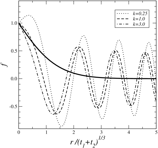
Figure 1: Scaling function $f(y)$ in the case $z=n=3$, normalised to $f(0)=1$. The solid line gives the behaviour if $\mu_{1}=1>0$, while the broken lines indicate the behaviour, for $\mu_{1}=-8<0$ and several values of $k$, of the function $f(y)=(\mbox{\rm Ai}(|\mu_{1}|^{1/3}y)+k\mbox{\rm Bi}(|\mu_{1}|^{1/3}y))/(\mbox{\rm Ai}(0))+k\mbox{\rm Bi}(0))$.

2. $n=4$. The solution of (4.9) now takes the more simple form

$$f(y)=f_{0}\>{}_{0}F_{2}\left(\frac{1}{2},\frac{3}{4};-\frac{\mu_{1}y^{4}}{64}\right)+f_{1}\,y\>{}_{0}F_{2}\left(\frac{3}{4},\frac{5}{4};-\frac{\mu_{1}y^{4}}{64}\right)+f_{2}\,y^{2}\>{}_{0}F_{2}\left(\frac{5}{4},\frac{3}{2};-\frac{\mu_{1}y^{4}}{64}\right)$$ (4.16)

This may be analysed using the leading asymptotic behaviour of the hyper-geometric function ${}_{0}F_{2}$, which may be read off from Wright’s formulæ [50]

$${}_{0}F_{2}(a,b;z) \stackrel{{\scriptstyle z\to\infty}}{{\simeq}} \frac{\Gamma(a)\Gamma(b)}{2\pi\sqrt{3\,}}\>z^{(1-a-b)/3}\;e^{3z^{1/3}}$$

$${}_{0}F_{2}(a,b;-z) \stackrel{{\scriptstyle z\to\infty}}{{\simeq}} \frac{\Gamma(a)\Gamma(b)}{\pi\sqrt{3\,}}\>z^{(1-a-b)/3}\;e^{3z^{1/3}/2}\cos\left(\frac{3\sqrt{3\,}}{2}z^{1/3}+\frac{\pi}{3}(1-a-b)\right)$$ (4.17)

For both $\mu_{1}>0$ and $\mu_{1}<0$, this implies that the function $f(y)$ diverges exponentially fast as $y\to\infty$. We absorb this divergence by choosing the constants $f_{0,1,2}$ accordingly and then find

$$f(y)=f_{0}\left[{}_{0}F_{2}\left(\frac{1}{2},\frac{3}{4};-\frac{\mu_{1}y^{4}}{64}\right)-\frac{\sqrt{2\,}\,\Gamma(3/4)}{\Gamma(1/2)}\mu_{1}^{1/4}y\>{}_{0}F_{2}\left(\frac{3}{4},\frac{5}{4};-\frac{\mu_{1}y^{4}}{64}\right)\right.$$

$$\left.+\frac{\Gamma(3/4)}{\Gamma(1/4)}\mu_{1}^{1/2}y^{2}\>{}_{0}F_{2}\left(\frac{5}{4},\frac{3}{2};-\frac{\mu_{1}y^{4}}{64}\right)\right] \mu_{1}>0$$ ; (4.18)

$$f(y)=f_{(0)}\bigl{[}{\cal F}_{1}(y)+k{\cal F}_{2}(y)\bigr{]}\hskip 216.2411pt \mu_{1}<0$$ ;

where $f_{0}$ and $f_{(0)}$ are normalisation constants, $k$ is a free parameter and

$${\cal F}_{1}(y) := |\mu_{1}|^{1/4}y\>{}_{0}F_{2}\left(\frac{3}{4},\frac{5}{4};\frac{|\mu_{1}|y^{4}}{64}\right)-\frac{\Gamma(1/2}{\Gamma(3/4)}\>{}_{0}F_{2}\left(\frac{1}{2},\frac{3}{4};\frac{|\mu_{1}|y^{4}}{64}\right)$$

$${\cal F}_{2}(y) := |\mu_{1}|^{1/2}y^{2}\>{}_{0}F_{2}\left(\frac{5}{4},\frac{3}{2};\frac{|\mu_{1}|y^{4}}{64}\right)-\frac{\Gamma(1/4}{\Gamma(3/4)}\>{}_{0}F_{2}\left(\frac{1}{2},\frac{3}{4};\frac{|\mu_{1}|y^{4}}{64}\right)$$ (4.19)

The behaviour of these scaling functions is illustrated in figure 2. We observe that once having eliminated the asymptotically leading term eq. (4.17), the physically required boundary condition $\lim_{y\to\infty}f(y)=0$ is satisfied.

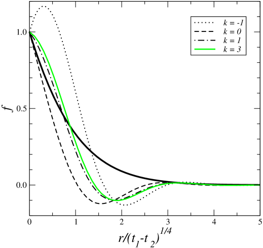
Figure 2: Scaling function $f(y)$ in the case $z=n=4$, normalised to $f(0)=1$. The thick solid line gives the behaviour if $\mu_{1}=1>0$. The broken lines and the grey line indicate the behaviour, for $\mu_{1}=-8<0$ and several values of $k$, of the function $f(y)=({\cal F}_{1}(y)+k{\cal F}_{2}(y))/({\cal F}_{1}(0)+k{\cal F}_{2}(0))$, with the ${\cal F}_{i}(y)$ defined in (4.19).

Comparing figures 1 and 2, we notice that although the scaling function satisfies for both $n$ odd and $n$ even the same differential equation (4.9), the interpretation of the scaling variable $|\mu_{1}|^{1/4}y$ is different. Indeed, for $n=3$, the time difference $t_{1}-t_{2}$ enters into $y$, whereas for $n=4$ it is the sum $t_{1}+t_{2}$. Furthermore, we see that for $\mu_{1}>0$, only a single independent solution remains, which decreases from $f(0)=1$ monotonously and very rapidly towards zero when $y$ is increased. On the other hand, for $\mu_{1}<0$, we find two independent admissible solutions whose decay towards zero is an oscillatory function of $y$ (for $n=3$, the decay should be algebraic, whereas it looks to be (stretched) exponential for $n=4$). This feature may allow to distinguish at least qualitatively between two physically distinct situations with $z>2$:

• non-equilibrium relaxation kinetics with a conserved order-parameter (model B dynamics). Below the critical point, viz. $T<T_{c}$, in systems with a global O($n$)-symmetry it is known that $z=3$ for a scalar order-parameter ($n=1$), and $z=4$ for vector order-parameters ($n\geq 2$) [9]. At criticality $z=4-\eta=4-\frac{1}{2}\frac{n+2}{(n+8)^{2}}\varepsilon^{2}+{\rm O}(\varepsilon^{3})$ in $d=4-\varepsilon$ dimensions [51]. In these cases, scaling functions are generically seen to be oscillating.

• in critical dynamics, viz. $T=T_{c}$, and without any conservation law on the order-parameter (model A dynamics), the dynamical exponent $z\gtrsim 2$ [51]. Here, the decay of the scaling functions is in general monotonous.

Our results suggest that these physically distinct cases, even with the same value of $z$, might be distinguished through the sign of the dimensionful parameter $\mu_{1}$, such that $\mu_{1}>0$ reproduces the monotonous decay seen in critical dynamics (model A) whereas $\mu_{1}<0$ leads to the oscillatory decay found in conserved systems (model B).

5 Conclusions

This work has been motivated by the persistent difficulties to construct non-trivial Lie algebras of space-time transformations. We believe that the possibility of finding Lie algebra generators which cannot be expressed as vector fields merits serious consideration. We have constructed new representations of the ageing algebra $\mathfrak{age}(1)$, corresponding to an integer dynamical exponent $z=n\geq 2$ to explore the mathematical structure of dynamical symmetries whose infinitesimal generators are no longer described by the usual vector fields involving only first-order differential operators. Provided that we restrict the admissible function space to the solution space of the Schrödinger equation ${\cal S}\psi=0$, and thereby somewhat relax the requirements of a dynamical symmetry, we have given an explicit $n$-dependent family of linear partial differential equations which are indeed $\mathfrak{age}(1)$-invariant in the sense introduced here. An important open question is how to extend this to non-linear equations.

The non-local infinitesimal generators of $\mathfrak{age}(1)$ contain higher-order differential operators. Their exponentiation does not lead to local spatio-temporal coordinate transformations and we have considered the possibility that a better interpretation might be formulated in terms of transformation rules for distributions of spatio-temporal coordinates. Several examples of such transformation rules have been derived.

Finally, we also studied the scaling form of co-variant two-point functions. Surprisingly, for $z=n$ even the scaling forms are compatible with the expectations of a two-time response function (as it is usually the case in present theories of local scale-invariance in ageing systems) since they depend on the time difference $t_{1}-t_{2}$. On the other hand, this is not so for $z=n$ odd, where the arguments of the scaling functions are much more reminiscent of co-variant two-time correlators, since they contain the sum $t_{1}+t_{2}$. We have also seen that the shape of the space-dependent part of the scaling functions can at least qualitatively account for the different forms found for non-conserved (model A) dynamics, where one expects a monotonous decay, and for conserved (model B) dynamics, where scaling functions are oscillatory.. This is achieved through a simple change in the sign of the dimensionful ‘mass parameter’ $\mu$. Although we think it unlikely that our non-local representations of $\mathfrak{age}(1)$ should be directly applicable to physical models, we consider this qualitative feature encouraging.

Appendix. On Galilei-transformations

For comparison with the non-local generators treated in the main text, we recall the computation of finite Galilei-transformations, for distributions with a non-vanishing mass $\mu\neq 0$. The infinitesimal generator is $Y_{1/2}=-t\partial_{r}-\mu r$, from which the finite transformation is formally obtained as $F(\varepsilon,t,r)=e^{-\varepsilon Y_{1/2}}F(0,t,r)$. It is given by the differential equation

$$\bigl{(}\partial_{\varepsilon}-t\partial_{r}-\mu r\bigr{)}F(\varepsilon,t,r)=0\;\;,\;\;F(0,t,r)=\phi(t,r)$$ (A.1)

where $\phi=\phi(t,r)$ denotes the given initial distribution. Eq. (A.1) is solved in Fourier space:

$$\widehat{\phi}(t,k)\mapsto\widehat{F}(\varepsilon,t,k)=\widehat{\phi}(t,k+{\rm i}\mu\varepsilon)\exp\left[-\frac{1}{2}\mu t\varepsilon+{\rm i}tk\varepsilon\right]$$ (A.2)

In direct space, the galilei-transformed distribution becomes

$$\phi(t,r)\mapsto F(\varepsilon,t,r) = \frac{1}{\sqrt{2\pi\,}\,}\int_{\mathbb{R}}\!{\rm d}k\>\widehat{\phi}(t,k+{\rm i}\mu\varepsilon)\,e^{{\rm i}k(r+t\varepsilon)}\,e^{\mu t\varepsilon^{2}/2}$$ (A.3)

$$= \frac{1}{2\pi}\int_{\mathbb{R}}\!{\rm d}r^{\prime}\>\phi(t,r)\,e^{\mu r^{\prime}\varepsilon-\mu t\varepsilon^{2}/2}\underbrace{\int_{\mathbb{R}}\!{\rm d}k\>e^{{\rm i}k(r-r^{\prime}+t\varepsilon)}}_{2\pi\delta(r+t\varepsilon-r^{\prime})}$$

$$= \phi(t,r+t\varepsilon)\,e^{\mu(r+t\varepsilon)\varepsilon-\mu t\varepsilon^{2}/2}$$

Hence, for $\mu=0$, the initial distribution is rigidly shifted according to $t\mapsto t$ and $r\mapsto r+t\varepsilon$. This is a consequence of the local nature of the standard Galilei-transformation, which can be expressed in terms of a vector field. In particular, the entries in table 1 are recovered.

Acknowledgements: Most of the work on this paper was done during the visits of S.S. at the Université Henri Poincaré Nancy I. S.S. is supported in part by the Bulgarian NSF grant DO 02-257.

References

• [1] A. Bagchi and I. Mandal, Phys. Lett. B675, 393 (2009).
• [2] A. Bagchi, R. Gopakumar, I. Mandal and A. Miwa, arxiv:0912.1090.
• [3] A. Bagchi and R. Gopakumar, J. High-energy Phys. 0907:307 (2009).
• [4] K. Balasubramanian and J. McGrevy, Phys. Rev. Lett. 101, 061601 (2008).
• [5] V. Bargman, Ann. of Math. 56, 1 (1954).
• [6] F. Baumann, S. Stoimenov and M. Henkel, J. Phys. A39, 4095 (2006).
• [7] F. Baumann and M. Henkel, J. Stat. Mech. P01012 (2007).
• [8] F. Baumann, S.B. Dutta, and M. Henkel, J. Phys. A: Math. Gen. 40, 7389 (2007).
• [9] A.J. Bray, Adv. Phys. 43, 357 (1994).
• [10] S.A. Cannas, D.A. Stariolo and F.A. Tamarit, Physica A294, 362 (2001).
• [11] R. Cherniha and M. Henkel, J. Math. Anal. Appl. at press (2010) (arxiv:0910.4822).
• [12] L.F. Cugliandolo, in Slow Relaxation and non equilibrium dynamics in condensed matter, Les Houches Session 77 July 2002, J-L Barrat, J Dalibard, J Kurchan, M V Feigel’man eds, Springer(Heidelberg 2003) (cond-mat/0210312).
• [13] X. Durang and M. Henkel, J. Phys. A: Math. Theor. 42, 395004 (2009).
• [14] C. Duval and P.A. Horváthy, J. Phys. A: Math. Theor. 42, 465206 (2009).
• [15] C.A. Fuertes and S. Moroz, Phys. Rev. D79, 106004 (2009).
• [16] C. Godrèche and J.M. Luck, J. Phys. A. Math. Gen. 33, 9141 (2000).
• [17] C. Godrèche and J.M. Luck, J. Phys. Cond. Matt. 14, 1589 (2002).
• [18] C. R. Hagen, Phys. Rev. D5, 377 (1972).
• [19] M. Hassaïne and P.A. Horváthy, Ann. of Phys. 282, 218 (2000); Phys. Lett. A279, 215 (2001).
• [20] P. Havas and J. Plebanski, J. Math. Phys. 19, 482 (1978).
• [21] M. Henkel, J. Stat. Phys. 75, 1023 (1994).
• [22] M. Henkel, Phys. Rev. Lett. 78, 1940 (1997).
• [23] M. Henkel, Nucl. Phys. B641, 405 (2002).
• [24] M. Henkel and J. Unterberger, Nucl. Phys. B660, 407 (2003).
• [25] M. Henkel, T. Enss and M. Pleimling, J. Phys. A Math. Gen. 39, L589 (2006).
• [26] M. Henkel, R. Schott, S. Stoimenov and J. Unterberger, preprint math-ph/0601028.
• [27] M. Henkel and M. Pleimling, Non-equilibrium phase transitions vol. 2: ageing and dynamical scaling far from equilibrium, Springer (Heidelberg 2010).
• [28] P. Hohenberg and B.I. Halperin, Rev. Mod. Phys. 49, 435 (1977).
• [29] P.A. Horváthy, L. Martina and P.C. Stichel, preprint arxiv:1002.4772.
• [30] E.V. Ivashkevich, J. Phys. A: Math. Gen. 30, L525 (1997).
• [31] R. Jackiw, Physics Today 25, 23 (1972).
• [32] J.I. Jottar, R.G. Leigh, D. Minic and L.A. Pando Zayas, preprint arxiv:1004.3752.
• [33] H.A. Kastrup, Nucl. Phys. B7, 545 (1968).
• [34] R.G. Leigh and N.N. Hoang, J. High-energy Phys. 0911:010 (2009).
• [35] R.G. Leigh and N.N. Hoang, J. High-energy Phys. 1003:027 (2010).
• [36] J. Lukierski, P.C. Stichel and W.J. Zakrewski, Phys. Lett. A357, 1 (2006); Phys. Lett. B650, 203 (2007).
• [37] D. Martelli and Y. Tachikawa, arxiv:0903.5184.
• [38] D. Minic and M. Pleimling, Phys. Rev. E78, 061108 (2008).
• [39] J. Negro, M.A. del Olmo and A. Rodríguez-Marco, J. Math. Phys. 38, 3786 and 3810 (1997).
• [40] U. Niederer, Helv. Phys. Acta 45, 802 (1972).
• [41] U. Niederer, Helv. Phys. Acta 51, 220 (1978).
• [42] L. O’Raifeartaigh and V.V. Sreedhar, Ann. of Phys. 293, 215 (2001).
• [43] L.V. Ovsiannikov, Group analysis of differential equations, Academic Press (New York 1982).
• [44] A. Picone and M. Henkel, Nucl. Phys. B688 217 (2004).
• [45] A. Röthlein, F. Baumann and M. Pleimling, Phys. Rev. E 74, 061604 (2006). Erratum E76, 019901 (2007).
• [46] C. Roger and J. Unterberger, Ann. Inst. H. Poincaré 7, 1477 (2006).
• [47] D.T. Son, Phys. Rev. D78, 106005 (2008).
• [48] S. Stoimenov and M. Henkel, Nucl. Phys. B723, 205 (2005).
• [49] S. Stoimenov, Fortschr. Phys. 57, 711 (2005).
• [50] E.M. Wright, J. London Math. Soc. 10, 287 (1935); and Proc. London Math. Soc. 46, 389 (1940); erratum J. London Math. Soc. 27, 256 (1952).
• [51] J. Zinn-Justin, Quantum field-theory and critical phenomena, 4th edition, Oxford University Press (2002).
• [52] P.-M. Zhang and P.A. Horváthy, Eur. Phys. J. C65, 607 (2010).