The Parker instability in axisymmetric filaments: final equilibria with longitudinal magnetic field

Se estudian los estados finales de equilibrio que surgen de la inestabilidad de Parker cuando partimos de una configuración cilíndrica de gas en equilibrio magnetohidrostático en un campo gravitacional radial y con un campo magnético longitudinal. Nuestro objetivo es comparar los estados de equilibrio no lineales con los que se obtienen en los sistemas con geometría Cartesiana. Se presentan los mapas de densidad y de las líneas de campo magnético en ambas geometrías para un campo gravitacional de intensidad constante. Encontramos que el flotamiento magnético es menos eficiente bajo simetría axial que en una atmósfera Cartesiana. Como consecuencia, las condensaciones que se forman en el modelo axisimétrico tienen menor densidad columnar. Por ende, el cociente entre la presión magnética y térmica en el estado final toma valores más extremos bajo simetría Cartesiana. Se discuten también algunos modelos en los que el campo gravitacional no es uniforme.

Abstract

We study the final equilibrium states of the Parker instability arising from an initially unstable cylindrical equilibrium configuration of gas in the presence of a radial gravitational field and a longitudinal magnetic field. The aim of this work is to compare the properties of the nonlinear final equilibria with those found in a system with Cartesian geometry. Maps of the density and magnetic field lines, when the strength of the gravitational field is constant, are given in both geometries. We find that the magnetic buoyancy and the drainage of gas along field lines are less efficient under axial symmetry than in a Cartesian atmosphere. As a consequence, the column density enhancement arising in gas condensations in the axially-symmetric model is smaller than in Cartesian geometry. The magnetic-to-gas pressure ratio in the final state takes more extreme values in the Cartesian model. Models with non-uniform radial gravity are also discussed.

0.1 Introduction

Parker (1966) demonstrated that a layer that is supported against the vertical gravity by the pressure of interstellar gas, horizontal magnetic field and cosmic rays, is always unstable to long wavelength deformations of the field lines because of the buoyancy of magnetic field and cosmic rays. Much work has been done to understand the role of the Parker instability in modeling the structure of the interstellar medium (ISM) and, more specifically, its role in gathering gas to trigger the formation of giant molecular clouds (e.g., Mouschovias et al. 1974; Blitz & Shu 1980; Mouschovias et al. 2009). Giz & Shu (1993), Kim et al. (1997) and Kim & Hong (1998) examined how the non-uniform nature of the Galactic gravity might affect the length and timescales of the Parker instability. Many studies have been devoted to investigate the effect of other physical ingredients on the Parker instability (Shu 1974; Nakamura et al. 1991; Hanawa et al. 1992; Hanasz & Lesch 2000; Kim et al. 2000; Santillán et al. 2000; Kim et al. 2001; Franco et al. 2002; Kosiński & Hanasz 2006, 2007; Lee & Hong 2007; Mouschovias et al. 2009).

The structure of the final static state resulting from the Parker instability was derived by Mouschovias (1974, hereafter M74) in the Cartesian model, namely, for a non-rotating layer under a vertical gravity, with a horizontal magnetic field in the initial equilibrium state. In the unperturbed state, the gas is in hydrostatic equilibrium in a stratified layer, so that all the quantities depend only on the distance from the midplane $y$, and the magnetic field is plane-parallel and runs along the $x$-direction. In this two-dimensional Cartesian problem, one assumes that all the quantities are independent of the third dimension, $z$, at any time. In the final state, the magnetic field rises in certain regions and sink in others forming bulges and valleys. Matter loads onto the field lines by draining down from the top region of the bulge and sinking into the valleys. So far, the final states of the Parker instability have been discussed in Cartesian models. In various astrophysical systems, however, the gas tends to form structures with other symmetries, such as filaments or elongated structures (e.g., Genzel & Stutzki 1989; Alfaro et al. 1992; Ryu et al. 1998; Conselice et al. 2001; Salomé et al. 2006; Jackson et al. 2010). Suppose now that we have a very elongated self-gravitating filamentary structure with a magnetic field traveling along the major axis of this structure, such that it has the effective geometry of a infinite cylinder. If the filament is supported against the radial self-gravity of the system by the pressure of gas and the longitudinal magnetic field, long wavelengths deformations of the magnetic field lines will allow matter to slide radially along field lines under the action of the gravitational field towards the symmetry axis, whereas the magnetic field tends to expand in radius, through a process of magnetic buckling (see Fig. 1). If the disturbances are axisymmetric, we expect the alternate formation of magnetic bottlenecks in the condensations of gas separated by portions of inflated magnetic lines or arcades, resembling a sausage mode. The final state is expected to be different than in a vertically stratified disk as those models currently used to study the Parker instability in galactic disks. In fact, the response of the system and the final equilibrium state depend on the adopted model: Cartesian or axisymmetric.

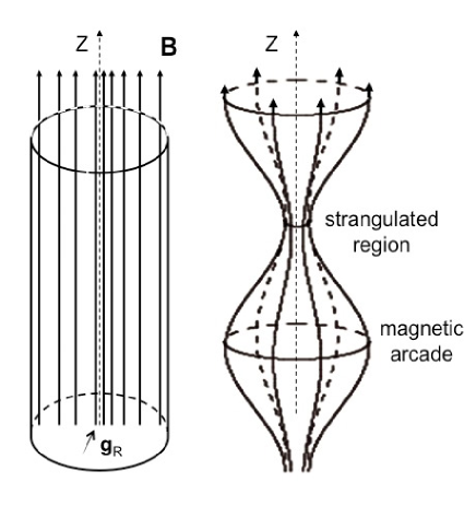
Figure 1: Sketch of the magnetic field configuration in the initial (left panel) and final (right panel) equilibrium states in axial symmetry.

In this paper, we study the nonlinear final equilibria of the Parker instability of a non-rotating, cylindrical initial state. In the initial state, the magnetic field is assumed to be parallel to the axis of the cylinder, which is taken to coincide with the $z$-axis. The cylinder is supported against the action of a radial gravitation field $g_{R}$ by the thermal and magnetic pressures (see Fig. 1). We will assume that the gas is isothermal and evolves under flux-freezing conditions. For axisymmetric perturbations, all the quantities only depend on $z$ and $R$ (not on the azimuthal angle $\phi$) and hence the problem is also two-dimensional. The evolution of the Parker instability in the $(z,R)$-plane is expected to be qualitative analogous in the main features, to the evolution found in the $(x,y)$-plane for the case of a plane-parallel initial state by M74. Throughout the paper, we will use the coordinate $z$ to denote the distance on the axis of symmetry in the axisymmetric model and should not be confused with the third component of the Cartesian model.

The aim of this work is to compare in detail how the final distributions of density and magnetic field vary from Cartesian to axisymmetric geometry. Accurate predictions of the nonlinear final states, an interesting problem in itself, can be very useful for the purpose of testing MHD codes. We will follow Mouschovias’ procedure (1974, 1976) to construct the final equilibrium states. Nakano (1979) and Tomisaka et al. (1988) used the same technique to find the structure of axisymmetric magnetized clouds that can be reached from nonequilibrium spherical configurations. By contrast, we start from a cylindrical configuration in magnetohydrostatic equilibrium as those used to study the gravitational collapse and fragmentation of filamentary clouds (e.g., Nakamura et al. 1995). In these simulations, however, the gravitational instabilities play a dominant role and not the Parker instability itself. In order to isolate the outcomes of the Parker instability, we will not consider self-gravity of the gas. In addition, we will also ignore the destabilizing influence of the interchange mode and the magnetic field curvature in the equilibrium states (Asséo et al. 1978, 1980; Lachièze-Rey et al. 1980), which could lead to the development of substructure. The study of these instabilities requires a full magnetohydrodynamical model and they will not be discussed further here.

Our paper is organized as follows. In Section 0.2, we describe the initial equilibrium configurations. The elliptic differential equations that give the equilibrium states under flux-freezing conditions are provided in Section 0.3. In Section 0.4 we compare the resulting features of the final states arising from the Parker instability in Cartesian and axisymmetric models. A summary of the results are presented in Section 0.5.

0.2 Initial states

We consider first the initial state in the Cartesian model, that is, a planar layer that is supported against the vertical gravity field by the gas pressure $P$ and a horizontal magnetic field. We will use a Cartesian coordinate system $(x,y)$, where $x$ is the horizontal coordinate and $y$ is the distance to the midplane of the layer, so that $\vec{B}_{0}=(B_{0,x}(y),0)$ in the initial state. Throughout the paper, the subscript $0$ signifies the initial state. Magnetohydrostatic equilibrium is satisfied if

$$\vec{\nabla}\left(P_{0}+\frac{B_{0,x}^{2}}{8\pi}\right)=-\rho\vec{\nabla}\psi,$$ (1)

where $\psi=\psi(y)$ is the gravitational potential. If the gas is isothermal with thermal sound speed $c_{s}$ and the ratio of the magnetic to gas pressures, $\alpha\equiv B_{0}^{2}/8\pi P_{0}$, is constant, the equilibrium equation reads

$$(1+\alpha)c_{s}^{2}\vec{\nabla}\ln\rho_{0}=-\vec{\nabla}\psi,$$ (2)

which has the solution

$$\rho_{0}(y)=\rho_{0}(0)\exp\left(-\frac{\psi}{(1+\alpha)c_{s}^{2}}\right),$$ (3)

with $\psi(0)=0$. If the gravitational field $\vec{g}=-\vec{\nabla}\psi$ is taken to be vertical and constant (but it reverses its direction across the midplane), we have $\psi=g|y|$, with $g={\rm constant}>0$. In this particular case, the mass density decays exponentially with a typical scale $H$ of $(1+\alpha)c_{s}^{2}/g$, whereas the magnetic field strength decays with a characteristic scale $2H$.

If, instead of a planar atmosphere, we assume that the gas extends to infinity along a cylinder whose axis coincides with the $z$-axis, and is threaded by an axial magnetic field $B_{z}$, the density profile at equilibrium is:

$$\rho_{0}(R)=\rho_{0}(0)\exp\left(-\frac{\psi}{(1+\alpha)c_{s}^{2}}\right),$$ (4)

where $R$ is the radial distance in cylindrical coordinates and $\psi(R)$ is the gravitational potential, with $\psi(0)=0$. In fact, we assume that the gravitational acceleration has only a radial component. If the radial gravitational force is taken to be constant, it holds that $\psi=gR$. Therefore, the radial scalelength for the density is $H=(1+\alpha)c_{s}^{2}/g$, as in Cartesian geometry.

We see that if the gravitational potential $\psi(y)$ in the infinite planar layer is identical to the gravitational potential $\psi(R)$ in the cylindrical model, the profiles of density, magnetic field and gas pressure along $y$ and $R$ will be identical in both models. However, these systems are no longer equivalent when the Parker instability arises. In the Cartesian model, magnetic field lines are allowed to inflate only in the vertical direction, whereas the expansion of field lines as well as the contraction of matter occur radially in the axisymmetric model (see Fig. 1). The question that arises is how the distributions of density, pressure and field lines in an azimuthal section [i.e. in the $(z,R)$-plane] look like as compared to those found in a vertical section [i.e. in the $(x,y)$-plane] in the well-studied Cartesian model.

When studying the Parker instability at the solar neighborhood, it is common to use a local Cartesian frame where the azimuthal direction is identified with the horizontal coordinate $x$ and the vertical direction of the Galaxy with $y$. In the two-dimensional approximation, the third radial direction is ignored. As a cautionary comment, our coordinate $R$ used throughout the paper should not be confused with the radial direction of the Galaxy.

0.3 The equilibrium equations

If a disturbance of sufficiently long wavelength is applied along the initial magnetic field to the initial equilibrium states described in the previous Section, the Parker instability develops in time and parts of the magnetic field lines bulge outward until the tension of the field lines increases sufficiently for an equilibrium state to be established. In the final states arising from the Parker instability, the magnetic field lines are curved and the magnetohydrostatic force equation is

$$-\vec{\nabla}P-\rho\vec{\nabla}\psi+\frac{1}{c}\vec{J}\times\vec{B}=0,$$ (5)

where $\vec{J}$ is the current density. The coordinate symmetries of the unperturbed states (see Section 0.2) reduce the problem to the $(x,y)$-plane in the Cartesian model and to the $(z,R)$-plane in the axisymmetric model. Under these symmetries, flux-freezing allows to transform the magnetostatic equations of equilibria into a second-order elliptic partial differential equation (Dungey 1953), conventionally called the Grad-Shafranov equilibrium equation. The beauty of this approach is that the final equilibrium states can be found with no need to solve a time-dependent problem (M74; Mouschovias 1976). In the following we give the Grad-Shafranov equilibrium equations and the boundary conditions. Details on its derivation can be found in M74, Mouschovias (1976) and Nakano (1979).

0.3.1 The Cartesian model

In the Cartesian layer with one ignorable coordinate, so that all quantities depend only on $(x,y)$, the magnetic vector potential can be written as ${\vec{A}}=A(x,y)\hat{e}_{z}$ and then $B_{x}=\partial A/\partial y$ and $B_{y}=-\partial A/\partial x$. One can show that the scalar function $q(x,y)$, defined by

$$q=P\exp\left(\frac{\psi}{c_{s}^{2}}\right),$$ (6)

is constant on a field line at magnetohydrostatic equilibrium, and is given by:

$$q(A)=\frac{c_{s}^{2}}{2}\frac{d\tilde{m}}{dA}\left[\int_{0}^{\lambda_{x}/2}\!\!\!\!dx\frac{\partial y(x,A)}{\partial A}\exp\left(-\frac{\psi(x,A)}{c_{s}^{2}}\right)\right]^{-1},$$ (7)

where $\lambda_{x}$ is the perturbation wavelength along the initial magnetic field and $d\tilde{m}$ is the mass per unit length (along the ignorable coordinate) in a flux tube between field lines characterized by $A$ and $A+dA$ and between $x=0$ and $x=\lambda_{x}$ (i.e. the mass-to-flux ratio). Under flux-freezing conditions, the mass-to-flux ratio is a constant of motion and, therefore, can be determined from the initial equilibrium configuration:

$$\frac{d\tilde{m}}{dA}=\lambda_{x}\frac{\rho_{0}(A)}{B_{0}(A)}.$$ (8)

Finally, the magnetic equilibrium equation (5) may be written in terms of $A$ as

$$\nabla^{2}A=-4\pi\frac{dq}{dA}\exp\left(-\frac{\psi}{c_{s}^{2}}\right)$$ (9)

(Dungey 1953; M74). Once the boundary conditions are specified, Equations (7) and (9) can be solved numerically by using a iterative scheme (M74).

The boundary conditions we take are the same as those in M74. The system is assumed to be periodic in $x$ and symmetric about the $x$-axis so that Equation (9) is solved in the rectangle $0<x<X_{\rm max}$ with $X_{\rm max}=\lambda_{x}/2$ and $0<y<Y_{\rm max}$, with the boundary conditions

$$\frac{\partial A}{\partial x}\bigg{|}_{x=0,X_{\rm max}}=0.$$ (10)

The upper boundary must be far enough from the midplane not to affect the evolution since a small vertical size of the computational domain suppresses the instability (e.g., M74; Mouschovias 1996). At the upper boundary we impose that the field lines are not deformed, $A(x,Y_{\rm max})=A_{0}(Y_{\rm max})$. Due to the imposed reflection symmetry about the midplane, the field line originally coinciding with the $x$-axis remains undeformed.

In the following, we provide the equations for the particular case of a constant external field. Although a uniform acceleration is only realistic at high altitudes from the midplane, we will concentrate on this case for simplicity and to facilitate comparison with some previous work that use a constant gravitational field (e.g., M74; Mouschovias et al. 2009). A realistic model of the gravitational potential is important to derive the growth rate of the instability and the most unstable wavelength, which determines the separation of the magnetic valleys (Kim & Hong 1998; Section 0.4.2). For now, we are mainly interested in the main conceptual features that arise in the final equilibria state when the geometry of the problem is changed, even if the adopted spatial dependence of the gravitational field lacks a strong astrophysical motivation.

As said in Section 0.2, if the external gravitational field is constant, the gravitational potential is $\psi=g|y|$, with $g$ a positive and constant acceleration. The equations are put in dimensionless form by choosing the following natural units: $c_{s}^{2}/g$, $c_{s}$ and $\rho_{0}(0)$, for length, velocity and density, respectively, The magnetic vector potential will be measured in units of $-2HB_{0}(0)$. Note that the dimensionless vertical scale is $H=(1+\alpha)$ in these units. The dimensionless of Equation (9) has the form

$$\nabla^{2}A=\hat{Q}_{xy}(x,y;\alpha),$$ (11)

where

$$\hat{Q}_{xy}=-\frac{1}{8\alpha(1+\alpha)^{2}}\frac{dq}{dA}\exp(-y).$$ (12)

In these units,

$$q(A)=\frac{1}{2}\frac{d\tilde{m}}{dA}\left[\int_{0}^{\lambda_{x}/2}dx\frac{\partial y(x,A)}{\partial A}\exp[-y(x,A)]\right]^{-1},$$ (13)

where

$$\frac{d\tilde{m}}{dA}=-2\lambda_{x}(1+\alpha)A.$$ (14)

Under constant gravity condition, the vector potential in the plane-parallel unperturbed state is

$$A_{0}(y)=\exp\left(-\frac{y}{2(1+\alpha)}\right),$$ (15)

and the source term of Eq. (11) is

$$\hat{Q}_{xy}^{(i)}=\frac{1}{4(1+\alpha)^{2}}\exp\left(-\frac{y}{2(1+\alpha)}\right).$$ (16)

In this initial state, the relation between $A$ and $q$ is $A_{0}(q)=q^{-1/(2\alpha)}$ (see also M74).

0.3.2 The axisymmetric model

Now, we consider a three-dimensional geometry with axial symmetry about the $z$-axis and longitudinal magnetic field ($B_{\phi}=0$). The magnetic field is related to the potential vector $\vec{A}=A(z,R)\hat{e}_{\phi}$ by $B_{z}=R^{-1}\partial(RA)/\partial R$ and $B_{R}=-\partial A/\partial z$. Under axisymmetric disturbances, the magnetic flux $\Phi(R,z)\equiv RA$ is constant on a magnetic surface and is also a constant of the motion. In this geometry, the function $q$ defined in Eq. (7) is given by

$$q(\Phi)=\frac{c_{s}^{2}}{2\pi}\frac{dm}{d\Phi}\left[\int_{0}^{\lambda_{z}/2}\!\!\!\!dz\frac{\partial R^{2}(z,\Phi)}{\partial\Phi}\exp\left(-\frac{\psi(z,\Phi)}{c_{s}^{2}}\right)\right]^{-1},$$ (17)

where $\lambda_{z}$ is the longitudinal perturbation wavelength and $dm$ is the mass in a flux tube between $\Phi$ and $\Phi+d\Phi$ and between $z=0$ to $z=\lambda_{z}$. Again, $q$ is a constant along field lines in equilibrium configurations. Under flux-freezing conditions, the mass-to-flux ratio is a constant of the motion, which can be determined from the initial configuration by:

$$\frac{dm}{d\Phi}=2\pi\lambda_{z}\frac{\rho_{0}}{B_{0}}.$$ (18)

The balance of forces (Eq. 5) in the final magnetic configuration can be rewritten in terms of $\Phi$ as

$$\nabla^{2}\Phi-\frac{2}{R}\frac{\partial\Phi}{\partial R}=-4\pi R^{2}\frac{dq}{d\Phi}\exp\left(-\frac{\psi}{c_{s}^{2}}\right)$$ (19)

(Mouschovias 1976; Nakano 1979). Equation (19) together with Eq. (17) enable us to derive $\Phi(z,R)$ once the boundary conditions are specified. The magnetic field can be found just by simple derivation: $B_{z}=R^{-1}\partial\Phi/\partial R$ and $B_{R}=-R^{-1}\partial\Phi/\partial z$.

The computational domain is a rectangular box of $0<z<Z_{\rm max}$ and $0<R<R_{\rm max}$. Because of the symmetries of the initial and final states, the length of the computation box in the $z$-direction, $Z_{\rm max}$, is taken to be $\lambda_{z}/2$, half the wavelength of the perturbation. Periodicity in $z$ is translated to

$$\frac{\partial\Phi}{\partial z}\bigg{|}_{z=0,Z_{\rm max}}=0.$$ (20)

The definition of $\Phi$ means that $\Phi(0,z)=0$ at any time. Assuming that the deformation of field lines can be neglected on the surface of the cylinder, we impose that $\Phi(z,R_{\rm max})=\Phi_{0}(R_{\rm max})$.

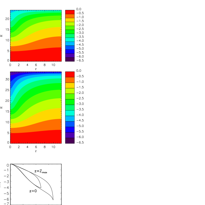
Figure 2: Azimuthal section of the magnetic flux $\Phi(z,R)$ in the axially-symmetric final state for $\alpha=1$ and $g_{R}=g={\rm const}$, when the upper boundary is placed at $R_{\rm max}=24$ (top) and at $R_{\rm max}=33.5$ (middle). Magnetic field lines coincide with the isocontours of $\Phi$. The color bar is in natural logarithmic scale. The unit length is $c_{s}^{2}/g$. A comparison of the radial profile of the magnetic flux along cuts at $z=0$ and $z=Z_{\rm max}$ is given in the lower panel when the boundary is at $R_{\rm max}=24$ and $R_{\rm max}=33.5$.

Figure 3: The shape of the function $q(A)$ (left panel) and $q(\Phi)$ (right panel) in the initial state (dashed lines) and in the final state (solid lines), with $\alpha=1$ and constant gravity, for $X_{\rm max}=15$ and $Z_{\rm max}=15$, respectively. Note that the range of the $q$-axis is different.

The equivalent condition of constant gravity is to assume that the radial gravitational field is constant, i.e. $\vec{g}=-g\hat{e}_{R}$, with $g$ a positive constant acceleration. We may use the same units for distance, velocity and density as those described in the previous subsection. The magnetic flux will be measured in units of $-4H^{2}B_{0}(0)$. Equation (19) in dimensionless form is:

$$\nabla^{2}\Phi-\frac{2}{R}\frac{\partial\Phi}{\partial R}=Q_{zR}(z,R;\alpha),$$ (21)

with

$$Q_{zR}=-\frac{R^{2}}{32\alpha(1+\alpha)^{4}}\frac{dq}{d\Phi}\exp\left(-R\right),$$ (22)

and

$$q(\Phi)=\frac{1}{2\pi}\frac{dm}{d\Phi}\left[\int_{0}^{\lambda_{z}/2}\!\!\!\!dz\frac{\partial R^{2}(z,\Phi)}{\partial\Phi}\exp\left[-R(z,\Phi)\right]\right]^{-1},$$ (23)

where the dimensionless mass-to-flux is

$$\frac{dm}{d\Phi}=-8\pi(1+\alpha)^{2}\lambda_{z}\frac{\rho_{0}}{B_{0}}$$ (24)

$$=-8\pi(1+\alpha)^{2}\lambda_{z}\exp\left(-\frac{R(\Phi)}{2(1+\alpha)}\right).$$ (25)

By comparing Eqs. (21)-(22) with Eqs. (11)-(12), we see that the dynamical variable $\Phi$ also satisfies a nonlinear elliptical differential equation, but with a different differential operator and source term than the equation governing $A$ in the Cartesian model.

In order to gain some physical insight, it is useful to compute the function $q(\Phi)$ in the initial equilibrium configurations which, of course, are solutions of the differential equation (21). In a model with uniform radial gravitational field, the magnetic flux and the $q$-function in the unperturbed state are, respectively:

$$\Phi_{0}(R)=\left(1+\frac{R}{2(1+\alpha)}\right)\exp\left(-\frac{R}{2(1+\alpha)}\right),$$ (26)

and

$$q_{0}(R)=\exp\left(\frac{\alpha R}{1+\alpha}\right).$$ (27)

At small enough $R$, say $R\ll 2(1+\alpha)$, they can be approximated by $\Phi_{0}(R)\approx\exp(-R/2[1+\alpha])$ and $q_{0}(\Phi_{0})=\Phi_{0}^{-2\alpha}$. Interestingly, they have exactly the same forms as $A_{0}(y)$ and $q_{0}(A)$ in the Cartesian model, respectively (see Eq. 15 and the very end of Section 0.3.1). At large radii, $R\gg 2(1+\alpha)$, or equivalently $\ln q\gg 2\alpha$, the relationship between $\Phi_{0}$ and $q_{0}$ is $\Phi_{0}\simeq(2\alpha)^{-1}q_{0}^{-1/(2\alpha)}\ln q_{0}$. Therefore, at these large $q$ values, $q$ increases with $\Phi^{-1}$ slightly faster than the rate at which $q$ increases with $A^{-1}$ in the Cartesian model ($q=A^{-2\alpha}$). In Section 0.4, we will calculate the dependence of the function $q$ on $\Phi$ in the final axially-symmetric equilibrium state. The shape of $q(\Phi)$ as compared to $q(A)$ in the Cartesian model will be also discussed.

Figure 4: The dependence of the functions $Q_{xy}$ and $Q_{zR}$ on $y$ and $R$, respectively in the initial states (dashed lines) and in the final states (solid lines), with $\alpha=1$ and constant gravity. In the left panels, $Q_{xy}$ is shown along the lines $x=0$ and $x=X_{\rm max}$ for two different wavelengths: $\lambda_{x}/2=9$ and $15$. The right panels display $Q_{zR}$ along the lines $z=0$ and $z=Z_{\rm max}$ for $\lambda_{z}/2=9$ and $15$, as quoted at the corners of these panels.

The source term of the differential equation in the initial cylindrical configuration with constant $g_{R}$ is:

$$Q_{zR}^{(i)}=\frac{1}{8(1+\alpha)^{3}}R\exp\left(-\frac{R}{2(1+\alpha)}\right).$$ (28)

By comparing Eqs. (16) and (28), we see that $Q_{zR}^{(i)}$ has a similar dependence on $R$ as $\hat{Q}_{xy}^{(i)}$ on $y$, except by the factor $R/(2+2\alpha)$. As a consequence, $Q_{zR}^{(i)}$ has a maximum at $2(1+\alpha)=2H$ whereas $\hat{Q}_{xy}^{(i)}$ is a monotonically decreasing function of $y$. In order to facilitate comparison between both cases, it is convenient to use $Q_{xy}$ defined as $Q_{xy}\equiv y\hat{Q}_{xy}/(2+2\alpha)$ because both $Q_{xy}$ and $Q_{zR}$ are identical at the initial state. However, they are expected to depart one from each other in the nonlinear equilibrium state because of the changes introduced by the different geometries. The form of $Q_{xy}$ and $Q_{zR}$ in the final equilibrium states will be discussed in the next Section.

0.4 Final equilibrium states

The final equilibrium state can be reached from the initial configuration through continuous deformations of field lines using a iterative method as described in M74. To do so, we add a perturbation to the magnetic variables in the initial equilibrium state,

$$\delta A(x,y)=-\mu A_{0}(y)\sin\left(\frac{\pi y}{Y_{\rm max}}\right)\cos\left(\frac{\pi x}{X_{\rm max}}\right),$$ (29)

for the Cartesian model and

$$\delta\Phi(z,R)=-\mu\Phi_{0}(R)\sin\left(\frac{\pi R}{R_{\rm max}}\right)\cos\left(\frac{\pi z}{Z_{\rm max}}\right),$$ (30)

for the axisymmetrical model. Here $\mu$ is the amplitude of the perturbation which we chose between $0.02$ and $0.06$. Note that the perturbations are symmetric about $y=0$ in the Cartesian model.

Our main interest is to compare the final equilibrium states in Cartesian and axisymmetrical models using the same external gravitational potential along $y$ and $R$, respectively. In this way, the comparison can be done on a common ground. In the next subsection, we will do so for models with constant gravitational acceleration. A more realistic gravitational potential will be studied in Section 0.4.2 in order to examine how it might affect the final nonlinear states.

0.4.1 Constant gravitational acceleration

Parker (1966) showed that a plane-parallel atmosphere with uniform gravity and a horizontal magnetic field is unstable to the undular mode if the horizontal wavelength of the perturbation is larger than a critical value, namely, $\lambda_{x}>\lambda_{\rm crit}\equiv 4\pi(1+\alpha)(2\alpha+1)^{-1/2}$. For the reference value $\alpha=1$, the dimensionless critical wavelength is $14.5$ or, equivalently, $7.26H$. Magnetic tension can stabilize disturbances with shorter wavelengths. The horizontal wavelength of the mode with the maximum growth rate depends on the vertical wavelength. For a typical value of $Y_{\rm max}=24$, the maximum growth rate occurs at $X_{\rm max}=12$ (i.e. $\lambda_{x}=24$).

The stability of magnetized cylinders has been considered in the past (e.g., Stodolkiewicz 1963; Nagasawa 1987) but, to our knowledge, none derived the dispersion relation under the assumption of constant gravitational field. Nevertheless, the linearized equations of motion under axial geometry and axisymmetric perturbations are identical to eqs. (III-3)-(III-6) quoted in Parker (1966), once the subscripts $y$ and $z$ in Parker’s notation are replaced for $z$ and $R$, except for the curvature term $v_{R}/R$ that appears as an extra term in the continuity and energy equations. Since the curvature term becomes small at scales comparable or larger than $\lambda_{\rm crit}$, the critical wavelength is essentially the same in both geometries. In fact, we have checked that our iterative scheme converges to the initial state as long as $\lambda_{z}\lesssim 7.5H$ (when $\alpha=1$ is used), indicating that they are stable.

In the Cartesian atmosphere, M74 found that if the upper boundary is far enough from the galactic plane, i.e. $Y_{\rm max}\gg(1+\alpha)$ in dimensionless units, the evolution of most of the matter in the domain is not affected by the location of the upper boundary. The reason is that more than $90\%$ of the energy of the initial state resides under $y<3.5(1+\alpha)$ (see M74). In the axisymmetrical model, we can apply the same reasoning to expect that the solution is not significantly altered as long as the box size is much larger than the effective scaleheight, defined as the radius $R$ at which $\Phi_{0}$ decays by a factor $e$, namely, $4.3(1+\alpha)$ [note that the effective scaleheight of $A_{0}$ in the Cartesian model is $2(1+\alpha)$]. In Figure 2 we compare the the magnetic flux of the final state in the axisymmetrical model using $\alpha=1$ and $\lambda_{z}/2=12$, when the upper boundary, $R_{\rm max}$, is located at $24$ and at $33.5$. We see that both maps are almost identical at $R<20$. The main difference is that upper magnetic field lines in the magnetic bulge region inflate further out when the boundary is far away because a larger column of material is unloaded and brought down to the valley of the curved magnetic field lines. Therefore, this upper region becomes lighter and more buoyant. By contrast, cuts of $\Phi$ along the valley $z=0$ are very similar in both cases (see the lower panel of Fig. 2). This means that the extra material that has been loaded into the valley when the upper boundary is placed at $33.5$, does not cause significant additional compression in the radial direction.

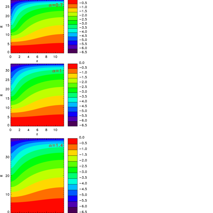
Figure 5: Color map of the magnetic flux $\Phi(z,R)$ in natural logarithmic scale for the final state for $\lambda_{z}/2=12$ (in dimensionless units) and different values of $\alpha$. The radial gravitational acceleration $g_{R}$ was assumed to be constant.

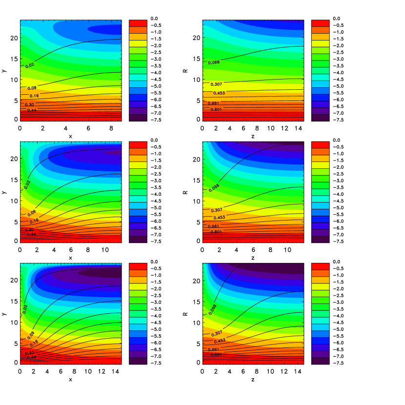
Figure 6: Contour plots of the density (color) and magnetic field lines (solid lines) for the Cartesian model (left) and the axisymmetric model (right), under constant gravity, for half the wavelength of $9,12$ and $15$ in units of $c_{s}^{2}/g$ (from top to bottom) and $\alpha=1$. The color bar gives the correlation between the colors and the natural logarithm of the density. The number on some curves is the value of $A$ in the Cartesian model or the value of $\Phi$ in the axisymmetric model. To make the comparison of the deformation of the magnetic field lines easier, we plot the same magnetic lines in both models.

In order to have the same dynamical range in all our calculations, we will place our upper boundary at the distance at which the variable of interest ($A$ for the Cartesian model and $\Phi$ for the axisymmetric case) decreases to $\exp(-6.12)=0.0022$ of its maximum value. With this convention, $Y_{\rm max}=12.2(1+\alpha)$ and $R_{\rm max}=16.7(1+\alpha)$. Interestingly, in the axisymmetric case, the corresponding density at $R_{\rm max}$ is only $5.4\times 10^{-8}$ of its value at $R=0$.

Different magnetostatic equilibrium configurations can be found by choosing the function $q(A)$ for the Cartesian model and $q(\Phi)$ for the axisymmetric one. Parker (1966) explored the cases in which $q(A)$ is either a linear or quadratic function of $A$. In practice, these functions are not free because they are defined by the initial conditions. M74 emphasized that $q$ increases when $A$ decreases in the Cartesian model. In Fig. 3, the functions $q(A)$ for the Cartesian layer and $q(\Phi)$ for the axially-symmetric configuration are plotted for $\alpha=1$ and $\lambda_{x}/2=\lambda_{z}/2=15$. In the initial state, the function $q_{0}(A)$ follows a power-law with index $-2\alpha$ (see Section 0.3.1 and Fig. 3). In the final equilibrium state, the power-law index varies with $A$, but $q(A)$ is always a monotonically decreasing function. As discussed in Section 0.3.2 and shown in Fig. 3, the slope of $q$ in the initial state of the axisymmetric model is steeper than in the Cartesian model. In fact, $q_{0}$ reaches a maximum value of $10^{7.3}$ in the axisymmetric model, but only $10^{6.2}$ in the Cartesian model. Note that the range of the $q$-axis in Fig. 3 was taken somewhat different in order to facilitate comparison of the shape of the curves. The behaviour of $q$ versus $\Phi$ in the final equilibrium state is similar as $q$ versus $A$ (see Fig. 3), although the new geometry introduces some remarkable differences in the shape of the function $q(\Phi)$. For instance, the change of $q$, relative to its initial value, in the range $0.6<\log_{10}\Phi^{-1}<1.5$ is smaller than in the same range of $A$ in the Cartesian model. The similar appearance of the functions $q(A)$ and $q(\Phi)$ should not lead us to the false conclusion that the source terms of the elliptic differential equations, namely $Q_{xy}(x,y)$ and $Q_{zR}(z,R)$, are also similar. Figure 4 displays $Q_{xy}$ at two different cuts along $x=0$ and $x=X_{\rm max}$, and $Q_{zR}$ along $z=0$ and $z=Z_{\rm max}$. The fractional change of $Q_{xy}$ from its initial value is always larger than the change of $Q_{zR}$. Both $Q_{xy}$ and $Q_{zR}$ may present two local maxima along a cut through the maximum heights of the magnetic field lines, i.e. along $x=X_{\rm max}$ and $z=Z_{\rm max}$. The relative amplitude of these maxima varies with the wavelength of the perturbation.

Figure 5 shows contour plots of the magnetic flux in the final axisymmetric state for a disturbance with $\lambda_{z}/2=12$ and three different $\alpha$ values ($\alpha=0.7,1.0$ and $1.4$). We see that the maps are a scaled version to each other by the factor $1+\alpha$. Since it is common for astrophysical purposes to assume equipartition between magnetic field and gas pressures, we will restrict ourselves to the case $\alpha=1$ hereafter.

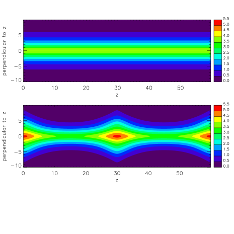
Figure 7: Column density map for the initial (top panel) and final axisymmetric state (bottom panel) along a line of sight perpendicular to the axis of symmetry ($z$-axis). We used $\alpha=1$, $\lambda_{z}/2=15$ and uniform radial gravity. The units of surface density and length are $\rho_{0}(0)c_{s}^{2}/g$ and $c_{s}^{2}/g$, respectively. Note that the scale is linear.

Figure 6 exhibits contour plots of the density (color) and magnetic field lines in the final stable state of the axisymmetric model for three different horizontal wavelengths ($\lambda_{z}/2=9,12$ and $24$). For comparison, density and magnetic field lines are also shown for the Cartesian model. Although the vertical size of the computational domain is larger in the axisymmetric case, we show the same box in all the cases for ease in visualization. When the systems are disturbed with the same wavelength, it is clear from Fig. 6 that the field lines and the density contours become more deformed in the Cartesian model than under axial symmetry. It turns out that a cylindrical initial configuration is more rigid to perturbations and the magnetic field is less buoyant than a plane-parallel layer. Interestingly, the same degree of deformation of magnetic field lines found for $\lambda_{x}/2=9$ in the Cartesian model, can be achieved in the axisymmetric case but for a longer wavelength of $\lambda_{z}/2=12$. Likewise, the level of radial buoyancy of the magnetic field for $\lambda_{z}/2=15$ is comparable to the level of vertical buoyancy for $\lambda_{x}/2=12$ in the Cartesian model.

The column density map of a filament with $\alpha=1$ and whose axis of symmetry lies in the plane of the sky is given in Fig. 7 in the initial and final equilibrium states with $\lambda_{z}/2=15$. The scaleheight of the column density along a condensation in the direction perperdicular to $z$ is about twice the scaleheight in the wings of the condensations. As a consequence of the less efficient drainage of gas into the magnetic valleys, the column density enhancement in the gas condensations is rather modest. In fact, the maximum enhancement in the column density over a line of sight with zero impact parameter, is smaller than in the Cartesian model (see Fig. 8). The column density may increase up to a factor of $7/4$ in Cartesian geometry (see also Kim et al. 2004) but only by a factor of $5/4$ in the axisymmetric model.

The result that a cylindrical configuration is more rigid than a plane-parallel layer has, a posteriori, a simple geometrical explanation as follows. Since magnetic forces act only perpendicular to the field lines, gas pressure gradients must balance the gravitational forces along a field line regardless the geometry of the problem. The plasma must slide down along the magnetic field lines until it reaches a new configuration of pressure equilibrium. The point is that, because of the radial convergence of the flow streamlines in the axisymmetrical model, we need less displacement of gas in the axisymmetric case than in the Cartesian model to achieve the same pressure gradient, as soon as the gas is isothermal, and, henceforth, less deformation of the magnetic field lines.

Figure 8: Column density for the final states as a function of the horizontal coordinate for $\lambda/2=15$ and constant gravity. In the Cartesion model, the column density is $\Sigma(x)=\int_{-\infty}^{\infty}\rho(x,y)dy$. In the axisymmetric model, we plot the column density along a line of sight perpendicular to the axis of symmetry and with null impact parameter, i.e. $\Sigma(z)=\int_{-\infty}^{\infty}\rho(z,R)dR$. The column density at the initial states is drawn as a dotted line.

Since the separation between magnetic field lines in azimuthal sections do not reflect the magnetic strength in the axisymmetric case, it is illustrative to compare the magnetic pressure to make a fair comparison between the results in Cartesian and axial geometries (see Fig. 9). Given a certain wavelength of the perturbation, the magnetic pressure maps depend on the geometry. Because of the stronger deformation in the Cartesian scenario, the magnetic pressure force and the magnetic stresses along the valleys of the magnetic field lines, i.e. at the cut $x=0$, are larger than along $z=0$. The distribution of magnetic pressure in the axial model with $\lambda_{z}/2=12$ is quite similar to the magnetic pressure configuration in the Cartesian case with $\lambda_{x}/2=9$.

The ratio of the magnetic to gas pressures is an indicator of the efficiency with which gas flows along field lines. As the increase of gas density in the magnetic field valleys is due primarily to the drainage along the field lines (see also M74), we expect that if the drainage is less efficient in the axisymmetrical case, the variation of $\alpha$ in the final state relative to the initial values should be also smaller. In Fig. 10, we plot the distribution of the magnetic-to-gas pressure ratio along $x=0$ and $x=X_{\rm max}$ for the Cartesian model, and along the same cuts $z=0$ and $z=Z_{\rm max}$ for the axisymmetric model in the final state, for a perturbation with half the wavelength of $15$. Although the general shape of the curves is rather similar in both geometries, the $\alpha$ values in the range $10<y<22$ at $x=X_{\rm max}$ are almost a factor $10$ larger than in the axisymmetric model at the same region (i.e. $10<R<22$ and $z=Z_{\rm max}$).

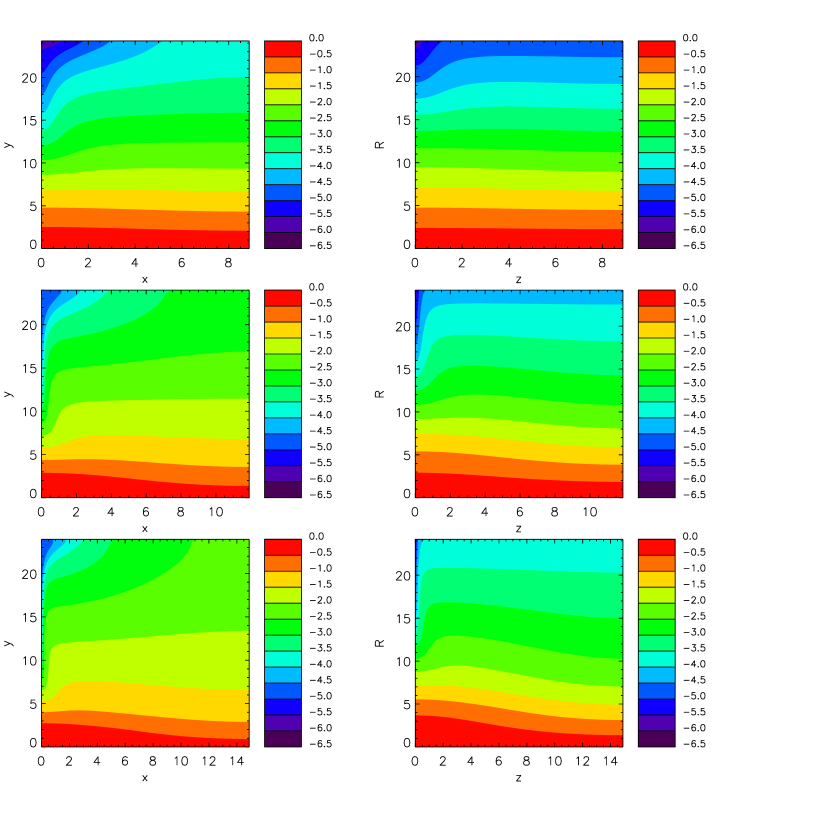
Figure 9: Magnetic pressure maps, normalized to its value on the $z$-axis in the initial state, in the six final states of Figure 6.

0.4.2 Non-uniform gravitational acceleration

In a infinite self-gravitating isothermal filament, the gravitational acceleration $g_{R}$ at large $R$ decays as $1/R$, whereas it increases linearly at small $R$. Therefore, the assumption that $g_{R}$ is constant is only valid at some intermediate range in $R$. To close our analysis, in this subsection we present the final equilibria for axially-symmetric configurations in a more realistic external gravitational field.

According to the results of Kim & Hong (1998) for a Cartesian model, the growth time is reduced by almost an order of magnitude and the length scale of the most unstable mode by factors of $4$–$8$ when a more realistic gravity model is used because in such a realistic disk the magnetic field strength decreases rapidly with vertical distance which promotes the development of strong magnetic buoyancy. We expect, therefore, that the length and timescales of the Parker instability in a filament will be modified if a more realistic gravity model is adopted.

In order to have a model as self-consistent as possible, we will assume that the external gravitational potential is dominated by a collisionless (stellar or dark matter) component with isothermal one-dimensional velocity dispersion $\sigma_{\star}$. The gravitational potential created by an isothermal filament is given by

$$\psi(R)=2\sigma_{\star}^{2}\ln\left(1+\frac{R^{2}}{8H_{\star}^{2}}\right),$$ (31)

where $H_{\star}$ is a parameter that specifies the scale height of the collisionless component satisfying $4\pi G\rho_{0,\star}(0)H_{\star}^{2}=\sigma_{\star}^{2}$, where $\rho_{0,\star}(0)$ is the density of collisionless matter at $R=0$ (e.g., Ostriker 1964). As already anticipated, the gravitational acceleration $g_{R}(R)$ increases linearly with $R$ at $R\ll\sqrt{8}H_{\star}$, reaches a maximum at $\sqrt{8}H_{\star}$ and decreases as $1/R$ at $R\gg\sqrt{8}H_{\star}$. Under this gravitational field, the density and magnetic field in the unperturbed state are:

$$\frac{\rho_{0}(R)}{\rho_{0}(0)}=\frac{B_{0}^{2}(R)}{B_{0}^{2}(0)}=\left(1+\frac{R^{2}}{8H_{\star}^{2}}\right)^{-s},$$ (32)

where $s$ is defined by $s\equiv 2\sigma_{\star}^{2}/[(1+\alpha)c_{s}^{2}]$. If we define the scale height of the gas, $H$, as the radial distance at which the density of the gas is reduced to $1/e$ of its value at $R=0$, then $H^{2}=8(\exp(1/s)-1)H_{\ast}^{2}$.

To illustrate the effect of using a non-constant gravitational acceleration, we useed $\alpha=1$ but different values of $s$. We ran models where the upper cap was located at the distance $R_{\rm max}$ at which the density decreases to $(1-5)\times 10^{-6}$ of its value at $R=0$. We have empirically derived that the larger the $s$-value is, smaller the critical wavelength becomes. For $s=4$, perturbations with $\lambda_{z}/2=3.85H_{\star}=2.55H$ are marginally unstable, whereas they become marginally unstable at $\lambda_{z}/2=1.5H$ when $s=8$. In terms of $H$, this result implies that the critical wavelength for $s=4$–$8$ is smaller by almost a factor of $1.5$–$2.5$ than that for the model with constant gravity (see Section 0.4.1) and, thereby, the growth timescale is shorter for larger $s$-values. Figure 11 shows the final equilibrium state for $s=4$ and $\lambda_{z}/2=5.3H$. This $\lambda_{z}$-value is close to the horizontal wavelength with maximum growth rate. By comparing with Figure 6, we note that although the global appearance is similar to the case with constant gravity and $\lambda_{z}/2=15$, the field lines appear slightly more deformed. The main effect of a non-constant gravitational acceleration strength is to shorten the separation of the magnetic valleys. The projected surface density that an observer would see if the axis of the filament lies in the plane of the sky is shown in Fig. 12 for a model with $s=4$. The enhancement in the column density over a line of sight passing through the core of a condensation is $2.1$ in this model. This factor is appreciably larger than that obtained in axisymmetric models with constant gravity but similar to that found in Cartesian models with uniform gravity.

0.5 Discussion and conclusions

The Parker instability dictates that longitudinal magnetic field lines that give some support against gravity are always unstable to undular perturbations. It has long been realized that the Parker instability, which is interesting in itself, may play a significant role to understand the formation of massive clouds in the interstellar medium, probably aided by thermal and gravitational instabilities (Mouschovias et al. 2009). The Parker instability can also play a role in the evolution of filamentary structure, such as filamentary clouds, at least at the early stages of the instability. While the properties of the final states are well documented for Cartesian models (e.g., M74; Basu et al. 1997; Kim et al. 2001), it was unclear how they depend on the adopted geometry. In order to fill this gap, our primary goal was to investigate the nonlinear outcome of such instability in an axisymmetric model where the initial equilibrium configuration consists of a infinite cylinder in the presence of a longitudinal magnetic field. We quantified the level of buoyancy of the magnetic field and drainage of the gas to promote density enhancements, as compared to the Cartesian models, which are currently being used to study the formation of substructure in the interstellar medium. We focused on understanding the physics of the Parker instability in filaments, rather than on making detailed comparisons with observations. This may be very useful as a first step to interpret full numerical simulations.

In the Cartesian model, the potential vector function $A$ obeys a nonlinear elliptic equation, while that for the axisymmetric model is the magnetic flux $\Phi$. However, the differential operator as well as the source terms are different. In order to gain some insight on the different nature of the equations, we have compared the form of $q(A)$ and $q(\Phi)$ at the initial and final states in each model. The source terms depend directly on the derivatives of these functions. However, in spite that the aspect of these functions looks like similar at a glance, the source terms $Q_{xy}$ and $Q_{zR}$ turn out to be absolutely different in the final state. This is a consequence of the nonlinearity of the differential equations.

We have focused first on models with uniform external gravity. We found that the axial model is more rigid than the Cartesian layer, in the sense that the magnetic field is less buoyant and the drainage of gas less efficient. In fact, in the axisymmetric model the matter shrinks in radius and generates a convergent flow that facilitates to achieve pressure equilibrium with less deformation of field lines. In order to have the same level of deformation of the field lines than in the Cartesian model with half the wavelength of $9c_{s}^{2}/g$, we need a perturbation of half the wavelength of $12c_{s}^{2}/g$, for $\alpha=1$. Under uniform gravity, we find that a factor $5/4$ enhancement in column density can be obtained in the axisymmetric model for the more unstable wavelength, which is modest as compared to the factor of $7/4$ found in the Cartesian model. At the position of the wings of the condensations, the ratio of the magnetic-to-gas pressures becomes larger than $1$ beyond a certain radius because of the evacuation of gas in these regions. However, it is still approximately $10$ times smaller than in Cartesian geometry.

We have examined a more realistic choice to describe the variation of the external gravitational potential in axisymmetric models. The main effects of a non-uniform gravitational acceleration is to modify the separation of magnetic valleys and thereof the timescale of the Parker instability. A factor of $2$ enhancement in column density over its initial equilibrium value can be found in axisymmetric models with non-uniform radial gravity. Hence, unless this density enhancement is sufficient to initiate thermal or gravitational instabilities, the Parker instability should be thought of as setting the stage upon which other small-scale processes will be modeling the structure and evolution of the filament.

Figure 10: Decadic logarithm of the ratio between the magnetic and gas pressures in the final state under constant gravity condition. The two solid lines give $\alpha$ values along the lines $x=0$ and $x=X_{\rm max}=15$ for the Cartesian model and the dashed lines give $\alpha$ along $z=0$ and $z=Z_{\rm max}=15$ in the axisymmetric case.

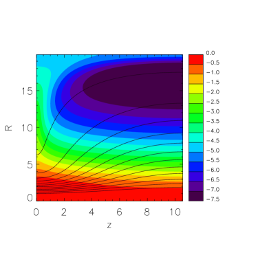
Figure 11: Distribution of the volume density and magnetic field lines in the axisymmetric final equilibrium state in a non-uniform radial gravitational field with $s=4$. In order to facilitate comparison with Fig. 6 in which $H=2$, distance is measured in units of $H/2$. Field lines (solid curves) were chosen so that they have the same magnetic strength in the initial state than those displayed in Fig. 6.

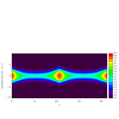
Figure 12: Column density map for the final axisymmetric state along a line of sight perpendicular to the axis of symmetry ($z$-axis). We used $\alpha=1$, $s=4$ and $\lambda_{z}=21.3$. The units of density and length are $\rho_{0}(0)$ and $H/2$, respectively. Note that the scale is linear.

References

- [Alfaro et al.(1992)] Alfaro, E. J., Cabrera-Caño, J., & Delgado, A. J. 1992, ApJ, 399, 576
- [Asséo et al.(1978)] Asséo, E., Cesarsky, C. J., Lachièze-Rey, M., & Pellat, R. 1978, ApJ, 225, L21
- [Asséo et al.(1980)] Asséo, E., Cesarsky, C. J., Lachièze-Rey, M., & Pellat, R. 1978, ApJ, 237, 752
- [Basu et al.(1997)] Basu, S., Mouschovias, T. Ch., & Paleologou, E. V. 1997, ApJ, 480, L55
- [Blitz & Shu(1980)] Blitz, L., & Shu, F. H. 1980, ApJ, 238, 148
- [Conselice et al.(2001)] Conselice, C. J., Gallagher III, J. S., & Wyse, R. F. G. 2001, ApJ, 122, 2281
- [Dungey(1953)] Dungey, F. W. 1953, MNRAS, 113, 180
- [Franco et al.(2002)] Franco, J., Kim, J., Alfaro, E. J., & Hong, S. S. 2002, ApJ, 570, 647
- [Genzel & Stutzki(1989)] Genzel, R., & Stutzki, J. 1989, ARA&A, 27, 41
- [Giz & Shu(1993)] Giz, A. T., & Shu, F. H. 1993, ApJ, 404,185
- [Hanasz & Lesch(2000)] Hanasz, M., & Lesch, H. 2000, ApJ, 543, 235
- [Hanawa et al.(1992)] Hanawa, T., Matsumoto, R., & Shibata, K. 1992, ApJ, 393, L71
- [Jackson et al.(2010)] Jackson, J. M., Finn, S. C., Chambers, E. T., Rathborne, J. M., & Simon, R. 2010, ApJ, 719, L185
- [Kim et al.(2000)] Kim, J., Franco, J., Hong, S. S., Santillán, A., & Matos, M. A. 2000, ApJ, 531, 873
- [Kim & Hong(1998)] Kim, J., & Hong, S. S. 1998, ApJ, 507, 254
- [Kim et al.(1997)] Kim, J., Hong, S. S., & Ryu, D. 1997, ApJ, 485, 228
- [Kim et al.(2004)] Kim, J., Ryu, D., & Hong, S. S. 2004, Ap&SS, 292, 255
- [Kim et al.(2001)] Kim, J., Ryu, D., & Jones, T. W. 2001, ApJ, 557, 464
- [Kosiński & Hanasz(2006)] Kosiński, R., & Hanasz, M. 2006, MNRAS, 368, 759
- [Kosiński & Hanasz(2007)] Kosiński, R., & Hanasz, M. 2007, MNRAS, 376, 861
- [Lachièze-Rey et al.(1980)] Lachiéze-Rey, M., Cesarsky, C. J., Asséo, E., & Pellat, R. 1980, ApJ, 238, 175
- [Lee & Hong(2007)] Lee, S. M., & Hong, S. S. 2007, ApJS, 169, 269
- [Mouschovias(1974)] Mouschovias, T. Ch. 1974, ApJ, 192, 37
- [Mouschovias(1976)] Mouschovias, T. Ch. 1976, ApJ, 206, 753
- [Mouschovias(1996)] Mouschovias, T. Ch. 1996, in Solar and Astrophysical Magnetohydrodynamic Flows, vol. 281, ed. K. C. Tsinganos, NATO ASI Ser. C (Kluwer, Dordrecht), p. 9
- [Mouschovias et al.(2009)] Mouschovias, T. Ch., Kunz, M. W., & Christie, D. A. 2009, MNRAS, 397, 14
- [Mouschovias et a.(1974)] Mouschovias, T. Ch., Shu, F. H., & Woodward, P. R. 1974, A&A, 33, 73
- [Nagasawa(1987)] Nagasawa, M. 1987, Progress of Theoretical Physics, 77, 635
- [Nakamura et al.(1991)] Nakamura, F., Hanawa, T., & Nakano, T. 1991, PASJ, 43, 685
- [Nakamura et al.(1995)] Nakamura, F., Hanawa, T., & Nakano, T. 1995, ApJ, 444, 770
- [Nakano(1979)] Nakano, T. 1979, PASJ, 31, 697
- [Ostriker(1964)] Ostriker, J. P. 1964, ApJ, 140, 1056
- [Parker(1966)] Parker, E. N. 1966, ApJ, 145, 811
- [Ryu et al.(1998)] Ryu, D., Kang, H., & Biermann, P. L. 1998, A&A, 335, 19
- [Salomé et al.(2006)] Salomé, P. et al. 2006, A&A, 454, 437
- [Santillán et al.(2000)] Santillán, A., Kim, J., Franco, J., Martos, M., Hong, S. S., & Ryu, D. 2000, ApJ, 545, 353
- [Shu(1974)] Shu, F. H. 1974, A&A, 33, 55
- [Stodolkiewicz(1963)] Stodolkiewicz, J. S. 1963, Acta Astronomica, 13, 30
- [Tomisaka et al.(1988)] Tomisaka, K., Ikeuchi, S., & Nakamura, T. 1988, ApJ, 335, 239