Abstract

We study the early-stage kinetics of thermodynamically unstable systems with quenched disorder. We show analytically that the growth of initial fluctuations is amplified by the presence of disorder. This is confirmed by numerical simulations of morphological phase separation (MPS) in thin liquid films and spinodal decomposition (SD) in binary mixtures. We also discuss the experimental implications of our results.

Introduction

There has been intense research interest in the kinetics of phase transitions in systems which have been rendered thermodynamically unstable by a sudden change of parameters, e.g., temperature, pressure, magnetic field, etc. The subsequent far-from-equilibrium evolution of the system is usually nonlinear, and is characterized by complex spatio-temporal pattern formation. The system approaches its new equilibrium state via the emergence and growth of domains enriched in the preferred phases. This nonequilibrium dynamics is often referred to as phase-separation kinetics or domain growth or coarsening or phase ordering dynamics [1]. These processes occur over a wide range of length-scales and time-scales, and are of great scientific and technological importance.

In pure (disorder-free) systems, the coarsening domains are usually characterized by a divergent length scale which grows as a power-law, $L(t)\sim t^{\phi}$, where the exponent $\phi$ depends on the transport mechanism. For example, in the phase separation of an unstable binary mixture via diffusion, $L(t)\sim t^{1/3}$ in the late stages of evolution. This is known as the Lifshitz-Slyozov (LS) growth law. In recent works [2, 3], we have established that the LS growth law also describes the late-stage dynamics in the morphological phase separation (MPS) of an unstable thin liquid film ($<100$ nm) on a solid substrate. During MPS, the film segregates into flat regions (domains) and high-curvature regions (defects or hills). In these works, we have also emphasized the analogies and differences between the kinetics of phase separation in binary mixtures and thin films.

Of course, real experimental systems are never pure or disorder-free: they are invariably characterized by chemical and physical heterogeneity [4, 5, 6, 7, 8, 9, 10, 11, 12, 13]. Therefore, it is natural to investigate the effects of disorder on the domain growth process. For segregating $AB$ mixtures, coarsening is driven by interfaces between coexisting $A$-rich and $B$-rich domains. These interfaces are trapped by sites of quenched disorder, and subsequent growth occurs by thermally-activated hopping of interfaces over disorder traps [14]. Thus, domain growth is drastically slowed down in the late stages, though the domain morphology is unaffected [15, 16, 17, 18]. On the other hand, unstable liquid films undergoing MPS segregate into regions with heights $h=h_{m}$ and $h=\infty$, i.e., there are no coexisting phases. The “interface” between the flat phase ($h=h_{m}$) and the high-curvature steepening phase ($h=\infty$) becomes sharper as time proceeds, and is unaffected by the presence of disorder. Thus, the asymptotic regime of MPS with disorder is universal, and is characterized by the LS growth law [3].

In this letter, we focus on the effect of disorder on the early stages of phase separation, i.e., the growth of small fluctuations about a homogeneous initial state. As we discuss shortly, both binary mixtures and thin films [19] are described by the Cahn-Hilliard-Cook (CHC) equation [20, 21] with appropriate free energies. The early-stage dynamics is described within the framework of a linear theory, usually referred to as CHC theory. In this letter, we report that growth in the CHC regime is strongly amplified by the presence of disorder. We present both analytical and numerical results to support this scenario. This should be contrasted with the late-stage dynamics, which is either slowed down (for binary mixtures) or unaffected (for thin films) by the presence of quenched disorder.

Dynamical Equations and Analytical Results

The starting point of our discussion is the dimensionless form of the CHC equation, which describes the evolution of a conserved order parameter $\psi(\vec{r},t)$ at space-point $\vec{r}$ and time $t$ [22]:

$$\frac{\partial}{\partial t}\psi(\vec{r},t)=\vec{\nabla}\cdot\left[M(\psi)\vec{\nabla}\left(\frac{\delta F[\psi]}{\delta\psi}\right)+\vec{\eta}(\vec{r},t)\right].$$ (1)

In Eq. (1), $M(\psi)$ is the mobility, and the Gaussian white noise $\vec{\eta}$ satisfies the fluctuation-dissipation relation:

$$\overline{\vec{\eta}(\vec{r},t)} = 0,$$

$$\overline{\eta_{i}(\vec{r}\,^{\prime},t^{\prime})\eta_{j}(\vec{r}\,^{\prime\prime},t^{\prime\prime})} = 2\epsilon M(\psi)\delta_{ij}\delta(\vec{r}\,^{\prime}-\vec{r}\,^{\prime\prime})\delta(t^{\prime}-t^{\prime\prime}).$$ (2)

Here, the bars denote an averaging over the noise ensemble, and $\epsilon$ measures the strength of the noise. Further, $F[\psi]$ is the free-energy functional which has the following form:

$$F[\psi]=\int d\vec{r}\left[f_{a}(\psi)+\frac{1}{2}{\left(\vec{\nabla}\psi\right)}^{2}\right].$$ (3)

In Eq. (3), $f_{a}(\psi)$ denotes the local free energy which is parameterized by the disorder strength $a$. The second term on the RHS refers to the interfacial energy or surface tension. Replacing Eq. (3) in Eq. (1), we obtain

$$\frac{\partial}{\partial t}\psi(\vec{r},t)=\vec{\nabla}\cdot\left[M(\psi)\vec{\nabla}\left\{f_{a}^{\prime}(\psi)-\nabla^{2}\psi\right\}+\vec{\eta}(\vec{r},t)\right].$$ (4)

The dimensionless Eqs. (1)-(4) are obtained from the corresponding dimensional equations by using the natural scales of length, time, and order parameter [1]. Before proceeding it is useful to discuss the functional form of $f_{a}(\psi)$ for the problems of interest here. For unstable thin films, $\psi$ is the height (usually denoted as $H$), and a typical form of $f_{0}(\psi)$ for the pure case ($a=0$) is

$$f_{0}(H)=-\frac{1}{6}\left[\frac{1-R}{\left(H+D\right)^{2}}+\frac{R}{H^{2}}\right].$$ (5)

This potential describes a thin film on a coated substrate. In Eq. (5), $R$ is the ratio of the effective Hamaker constants for the system, and $D$ is the dimensionless coating thickness. One can introduce the disorder in the coated potential through $R$ (chemically heterogeneous substrate) or $D$ (physically heterogeneous substrate). Here, we consider the case with chemical heterogeneity, so that $R$ is a $\vec{r}$-dependent random variable uniformly distributed in the interval $[R_{m}-a,R_{m}+a]$.

For segregating binary mixtures, $\psi$ denotes the density difference of the two species: $\phi(\vec{r},t)=n_{A}(\vec{r},t)-n_{B}(\vec{r},t)$, where $n_{\alpha}$ is the density of species $\alpha$. The local free energy for the disorder-free case is modeled by a $\phi^{4}$-potential with a double-well structure:

$$f_{0}(\phi)=-\frac{b\phi^{2}}{2}+\frac{\phi^{4}}{4},\quad b=1.$$ (6)

We model chemical heterogeneity by making $b$ a space-dependent random variable, which is uniformly distributed in $[1-a,1+a]$, i.e., the critical temperature varies from point to point.

Let us now return to Eq. (4). To understand the dynamics of the early stages, we consider the growth of initial fluctuations, $\psi(\vec{r},t)=\psi_{0}+\delta\psi(\vec{r},t)$. Here, $\psi_{0}$ is the homogeneous value of the order parameter in the unstable state. The linearization of Eq. (4) yields

$$\frac{\partial}{\partial t}\delta\psi(\vec{r},t)=M(\psi_{0})\nabla^{2}(-\alpha-\nabla^{2})\delta\psi+\vec{\nabla}\cdot\vec{\eta}(\vec{r},t),$$ (7)

where we have introduced the parameter $\alpha\equiv-f_{a}^{\prime\prime}(\psi_{0})$. We neglect terms involving the spatial derivatives of the disorder variable, as these are only relevant on microscopic scales. (We will subsequently average all physical quantities over the disorder distribution.) The Fourier transformation of Eq. (7) (with wave-vector $\vec{k}$) gives

$$\frac{\partial}{\partial t}\delta\psi(\vec{k},t)=M(\psi_{0})k^{2}(\alpha-k^{2})\delta\psi(\vec{k},t)-i\,\vec{k}\cdot\vec{\eta}(\vec{k},t),$$ (8)

which has the following solution:

$$\delta\psi(\vec{k},t) = \exp\left[M(\psi_{0})k^{2}(\alpha-k^{2})t\right]\delta\psi(\vec{k},0)$$ (9)

$$-i\,\vec{k}\cdot\int_{0}^{t}dt^{\prime}\exp\left[M(\psi_{0})k^{2}(\alpha-k^{2})(t-t^{\prime})\right]\vec{\eta}(\vec{k},t^{\prime}).$$

To obtain Eq. (9), we have set $M(\psi)\simeq M(\psi_{0})$ in Eq. (2), which is valid at early times. Clearly, averaging over the noise ensemble yields

$$\overline{\delta\psi}(\vec{k},t)=\exp\left[M(\psi_{0})k^{2}(\alpha-k^{2})t\right]\delta\psi(\vec{k},0).$$ (10)

The parameter $\alpha$ is spatially uniform for a chemically homogeneous system. For the disordered system, we have the local free energy

$$f_{a}(\psi)=f_{0}(\psi)+xf_{1}(\psi),$$ (11)

where $x$ is a uniformly-distributed random variable in the interval $[-a,a]$. For the disorder types we consider here, Eq. (11) is exact. Otherwise, it represents the first two terms of a Taylor expansion in the disorder $x$. Thus, $\alpha(x)=-f_{0}^{\prime\prime}(\psi_{0})-xf_{1}^{\prime\prime}(\psi_{0})$.

Finally, integrating Eq. (10) over the uniform disorder distribution with the probability $P(x)=1/(2a)$ gives

$$\widetilde{\delta\psi}(\vec{k},t)=\int_{-a}^{a}dx\,\frac{1}{2a}\exp\left[M(\psi_{0})k^{2}\left\{\alpha(x)-k^{2}\right\}t\right]\delta\psi(\vec{k},0).$$ (12)

Some simple algebra results in the following expression for the disorder-averaged growth of fluctuations:

$$\widetilde{\delta\psi}(\vec{k},t)=\exp\left[M(\psi_{0})k^{2}\left\{-f_{0}^{\prime\prime}(\psi_{0})-k^{2}\right\}t\right]\frac{\sinh[M(\psi_{0})f_{1}^{\prime\prime}(\psi_{0})k^{2}a\,t]}{M(\psi_{0})f_{1}^{\prime\prime}(\psi_{0})k^{2}a\,t}\,\delta\psi(\vec{k},0).$$ (13)

The factor $\sinh(ct)/(ct)$ determines the effect of disorder on the order-parameter evolution. This factor tends to 1 as $a\to 0$ or $k\to 0$ or $t\to 0$. However, the growth of initial fluctuations can be strongly amplified for nonzero $a$ as $\sinh(ct)$ grows exponentially with $t$.

Finally, we evaluate the time-dependent structure factor, which is probed in scattering experiments using, e.g., light, neutrons. This is defined as follows:

$$S(\vec{k},t)=\langle\delta\psi(\vec{k},t)\delta\psi^{*}(\vec{k},t)\rangle,$$ (14)

where the angular brackets indicate an averaging over thermal noise and independent initial conditions. Using the expression for $\delta\psi(\vec{k},t)$ from Eq. (9), we obtain

$$S(\vec{k},t)= A \!\!\!\!V\exp\left[2M(\psi_{0})k^{2}\left(\alpha-k^{2}\right)t\right]$$ (15)

$$+ \!\!\!\!\frac{\epsilon V}{\left(\alpha-k^{2}\right)}\left\{\exp\left[2M(\psi_{0})k^{2}\left(\alpha-k^{2}\right)t\right]-1\right\}.$$

To obtain Eq. (15), we assume that $\langle\delta\psi(\vec{r},0)\delta\psi^{*}(\vec{r^{\prime}},0)\rangle=A\delta(\vec{r}-\vec{r^{\prime}})$, where $A$ is the amplitude of initial fluctuations in the order parameter. Further, $V$ denotes the volume of the system. The corresponding disorder-averaged structure factor is

$$\widetilde{S}(\vec{k},t)= A \!\!\!\!V\exp\left[2M(\psi_{0})k^{2}\left\{-f_{0}^{\prime\prime}(\psi_{0})-k^{2}\right\}t\right]\frac{\sinh[2M(\psi_{0})f_{1}^{\prime\prime}(\psi_{0})k^{2}a\,t]}{2M(\psi_{0})f_{1}^{\prime\prime}(\psi_{0})k^{2}a\,t}$$ (16)

$$- \!\!\!\!\frac{\epsilon V}{2af_{1}^{\prime\prime}(\psi_{0})}\int_{-f_{0}^{\prime\prime}(\psi_{0})+af_{1}^{\prime\prime}(\psi_{0})-k^{2}}^{-f_{0}^{\prime\prime}(\psi_{0})-af_{1}^{\prime\prime}(\psi_{0})-k^{2}}dy\left\{\frac{\exp\left[2M(\psi_{0})k^{2}yt\right]-1}{y}\right\}.$$

Numerical Results

Next, we describe our numerical results for the chosen systems. For MPS in a thin film, the appropriate model is Eq. (4) with $\psi\equiv H$ and the local free energy:

$$f_{a}(H)=f_{0}(H)+xf_{1}(H),\quad f_{1}(H)=\frac{1}{6}\left[\frac{1}{(H+D)^{2}}-\frac{1}{H^{2}}\right],$$ (17)

where $f_{0}(H)$ is defined in Eq. (5). Here, we consider the case with mobility $M(H)=H^{3}$ (corresponding to Stokes flow with no slip) and $\epsilon=0$, i.e., without noise. We numerically solve Eq. (4) in $d=1$ starting with a small-amplitude ($\simeq 0.01$) random perturbation about the mean film thickness, $H_{0}=1$. The system size is $n\bar{L}_{M}$, where $\bar{L}_{M}$ is the dominant wavelength for $R=R_{m}$ ($n$ ranges from 16 to several thousands). We apply periodic boundary conditions at the end points. A 512-point grid per $\bar{L}_{M}$ was found to be sufficient when central-differencing in space with half-node interpolation was combined with Gear’s algorithm for time-marching, which is convenient for stiff equations. The parameters $D=0.5$, $R_{m}=-0.1$ and $a$ were chosen so that the film is spinodally unstable at $H=1$ (i.e., $\alpha>0$) for all values of $R$.

For segregation in a disordered binary mixture, we consider Eq. (4) with $\psi\equiv\phi$ and the free energy:

$$f_{a}(\phi)=f_{0}(\phi)+xf_{1}(\phi),\quad f_{1}(\phi)=-\frac{\phi^{2}}{2},$$ (18)

where $f_{0}(\phi)$ is defined in Eq. (6). We consider the case with $M(\phi)=1$ and $\epsilon=0$. We numerically solve Eq. (4) via an Euler-discretization scheme on a $d=2$ lattice of size $512^{2}$. The mesh sizes in space and time are $\varDelta x=0.5$ and $\varDelta t=0.001$, respectively. The spatial mesh size is small enough to resolve the interface region between $A$-rich ($\phi=+1$) and $B$-rich ($\phi=-1$) domains. The interface thickness $\xi\simeq\sqrt{2}$ in our dimensionless units. The initial condition for a run consists of small-amplitude ($\simeq 0.01$) fluctuations about $\phi_{0}=0$, corresponding to a critical $AB$ mixture with $50\%A$ and $50\%B$.

First, we present results for MPS in films with chemical heterogeneity. Recall that we are interested in the effect of disorder on the early stages of growth, i.e., the CHC regime. The height profiles at a fixed time ($t=4400$) for various disorder strengths are shown in Fig. 1(a). The initially random perturbations grow exponentially in time, with fastest growth for the case with maximum disorder ($a=0.04$). The growing fluctuations rapidly select the most unstable wavelength, $\lambda=\bar{L}_{M}$ – the location of the zero crossings is unaffected by the disorder. However, the peaks of the profiles are strongly amplified due to the factor $\sinh(ct)/(ct)$ in Eq. (13). This amplification may be quantitatively characterized by studying the statistical properties of the height profile. In Fig. 1(b), we plot $\widetilde{C}(0,t)=\langle\delta H(x,t)^{2}\rangle$ vs. $t$. This quantity is related to the structure factor in Eq. (14) as

$$\widetilde{C}(0,t)=\int\frac{d\vec{k}}{(2\pi)^{d}}\,\widetilde{S}(\vec{k},t),$$ (19)

where $d$ is the dimensionality. As expected, $\widetilde{C}(0,t)$ grows fastest for the case with maximum disorder.

The initial exponential growth of the profiles in the CHC regime is followed by a nonlinear saturation which results in the formation of domains of the flat phase, separated by defects of the high-curvature phase. These domains grow via the diffusive transport of material. The CHC regime and the domain growth regime are both shown in Fig. 2, where we plot the number of defects (hills) $N(t)$ vs. $t$. The characteristic length scale is $L(t)\sim N(t)^{-1}$. The CHC regime is followed by an intermediate stage where disorder sites trap the emergent interfaces. In this regime, the more disordered systems show slower growth. The intermediate stage is very sensitive to the presence of even small amounts of disorder. In the late stage, the domain growth is unaffected by disorder. In this regime, the interfaces (between $H=H_{m}$ and $H=\infty$) have steepened too much to be captured by the local disorder [3]. Thus, this regime shows universal LS growth [$N(t)\sim t^{-1/3}$ or $L(t)\sim t^{1/3}$]. This result has important experimental implications, viz., it is not necessary to work with specially-prepared extra-pure substrates, at least in the context of domain growth studies.

Next, we present our results for the early stages of spinodal decomposition (SD) in $d=2$ binary mixtures. In Fig. 3, we show the variation of the order parameter along a diagonal of the lattice ($y=x$). We plot profiles for the pure ($a=0$) and disordered ($a=0.5,0.8$) cases at $t=20$. Again, we see that there is an amplification of fluctuations for higher disorder values, though the selected wavelength does not change.

Finally, we study the structure factor $S(k,t)$ which provides a quantitative measure of the phase-separating morphology. In Fig. 4, we plot $S(k,t)$ vs. $k$ at $t=20$ for the pure and disordered cases shown in Fig. 3. In the early stages or the CHC regime, the structure factor grows exponentially in time but the peak position does not shift, i.e., there is no change in the characteristic scale. We see that the fastest growth occurs for the highest disorder amplitude. The solid lines in Fig. 4 denote the expression in Eq. (16) with $\epsilon=0$. Our numerical results are seen to be in excellent agreement with theory.

In the late stages of phase separation, disorder has the opposite effect, drastically slowing down domain growth [15, 16, 17, 18]. As stated earlier, this is because interfaces between coexisting $A$-rich and $B$-rich domains are trapped by sites of quenched disorder. This should be contrasted with the universal late-stage scenario for segregating films, as described above.

Summary and Discussion

In summary, we have studied the effect of quenched disorder on the early stages of evolution in two important systems: unstable thin films and phase-separating mixtures. Both these systems are described by the Cahn-Hilliard-Cook (CHC) equation with appropriate choices of the free energy. We find that disorder amplifies the exponential growth of fluctuations in the early CHC regime in both systems, and we have obtained a simple analytical expression for the amplification factor. In the asymptotic regime, there is a major difference between disordered domain growth in these two systems, viz., films undergoing MPS are unaffected by disorder, whereas segregating mixtures are drastically slowed down by disorder. Our results have important experimental consequences, and we hope that they will be subjected to experimental tests.

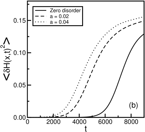
Figure 1: Early stages of morphological phase separation (MPS) in an unstable thin film with quenched disorder. (a) Height profiles [$H(x,t)$ vs. $x$] at $t=4400$ for different disorder amplitudes. The simulation details are provided in the text. (b) Plot of $\langle\delta H(x,t)^{2}\rangle$ vs. $t$ for the height profiles shown in (a).

Figure 2: Variation of the number density of defects with time [$N(t)$ vs. $t$] for MPS in an unstable thin film. Curves $1$ to $6$ present results for disorder amplitudes $a=0,0.0001,0.0004,0.002,0.01$ and $0.04$, respectively. The dashed lines with slopes of $-1/4$ and $-1/3$ denote exponents for the early and late stages, respectively [2, 3].

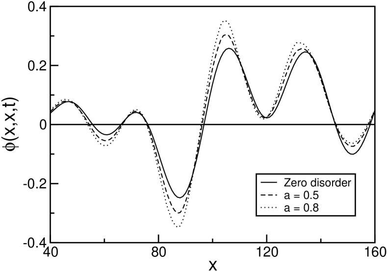
Figure 3: Early stages of spinodal decomposition (SD) in an unstable disordered binary mixture in $d=2$. The plot shows the variation of the order parameter along the diagonal [$\phi(x,x,t)$ vs. $x$] at $t=20$ for different disorder amplitudes. The simulation details are given in the text.

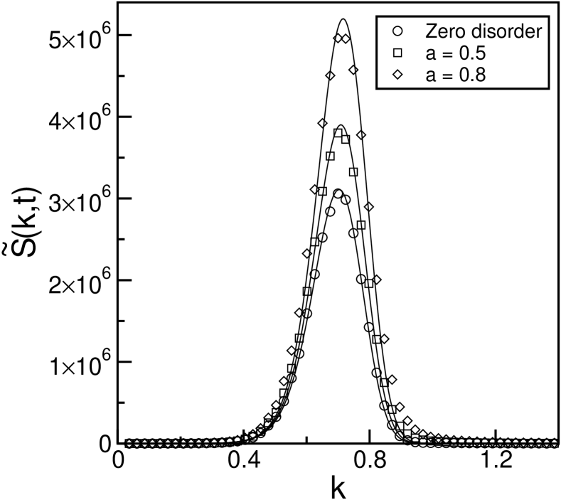
Figure 4: Plot of the spherically-averaged structure factor [$\widetilde{S}(k,t)$ vs. $k$] at $t=20$ for different disorder amplitudes. The structure factor is obtained as an average over 50 independent runs. The initial condition for each run consists of a different order parameter and disorder configuration. The solid lines denote the expression in Eq. (16) with $\epsilon=0$.

References

- [1] S. Puri and V. K. Wadhawan (eds.), Kinetics of Phase Transitions, CRC Press, Boca Raton, Florida (2009).
- [2] R. Khanna, N. K. Agnihotri, M. Vashishtha, A. Sharma, P. K. Jaiswal, and S. Puri, Phys. Rev. E 82, 011601 (2010).
- [3] M. Vashishtha, P. K. Jaiswal, R. Khanna, S. Puri, and A. Sharma, Phys. Chem. Chem. Phys. 12, 12964 (2010).
- [4] K. Kargupta, R. Konnur, and A. Sharma, Langmuir 16, 10243 (2000).
- [5] P. Volodin and A. Kondyurin, Journal of Physics D: Applied Physics 41, 065306 (2008).
- [6] P. Volodin and A. Kondyurin, Journal of Physics D: Applied Physics 41, 065307 (2008).
- [7] M. O. Robbins, D. Andelman, and J.-F. Joanny, Phys. Rev. A 43, 4344 (1991).
- [8] J. L. Harden and D. Andelman, Langmuir 8, 2547 (1992).
- [9] W. Koch, S. Dietrich, and S. Napiorkowski, Phys. Rev. E 51, 3300 (1995).
- [10] R. Lipowsky, P. Lenz, and P. S. Swain, Colloids and Surfaces A: Physicochemical and Engineering Aspects 161, 3 (2000).
- [11] H. Ikeda, Y. Endoh and S. Itoh, Phys. Rev. Lett. 64, 1266 (1990).
- [12] V. Likodimos, M. Labardi and M. Allegrini, Phys. Rev. B 61, 14440 (2000).
- [13] V. Likodimos, M. Labardi, X. K. Orlik, L. Pardi, M. Allegrini, S. Emonin and O. Marti, Phys. Rev. B 63, 064104 (2001).
- [14] D. A. Huse and C. L. Henley, Phys. Rev. Lett. 54, 2708 (1985).
- [15] S. Puri, Phase Transitions 77, 469 (2004).
- [16] S. Puri, D. Chowdhury, and N. Parekh, J. Phys. A 24, L1087 (1991); S. Puri and N. Parekh, J. Phys. A 25, 4127 (1992).
- [17] R. Paul, S. Puri, and H. Rieger, Europhys. Lett. 68, 881 (2004); Phys. Rev. E 71, 061109 (2005).
- [18] E. Lippiello, A. Mukherjee, S. Puri, and M. Zannetti, Europhys. Lett. 90, 46006 (2010).
- [19] V. S. Mitlin, J. Colloid Interface Sci. 156, 491 (1993).
- [20] J. W. Cahn and J. E. Hilliard, J. Chem. Phys. 28, 258 (1958).
- [21] H. E. Cook, Acta Metall. 18, 297 (1970).
- [22] P.C. Hohenberg and B.I. Halperin, Rev. Mod. Phys. 49, 435 (1977).