Nonparametric Bayesian sparse factor models with application to gene expression modeling

Abstract

A nonparametric Bayesian extension of Factor Analysis (FA) is proposed where observed data $\mathbf{Y}$ is modeled as a linear superposition, $\mathbf{G}$, of a potentially infinite number of hidden factors, $\mathbf{X}$. The Indian Buffet Process (IBP) is used as a prior on $\mathbf{G}$ to incorporate sparsity and to allow the number of latent features to be inferred. The model’s utility for modeling gene expression data is investigated using randomly generated data sets based on a known sparse connectivity matrix for E. Coli, and on three biological data sets of increasing complexity.

and

t1Supported by Microsoft Research through the Roger Needham Scholarship at Wolfson College, University of Cambridge. t2Supported by EPSRC Grant EP/F027400/1.

1 Introduction

Principal Components Analysis (PCA), Factor Analysis (FA) and Independent Components Analysis (ICA) are models which explain observed data, $\mathbf{y}_{n}\in\mathbb{R}^{D}$, in terms of a linear superposition of independent hidden factors, $\mathbf{x}_{n}\in\mathbb{R}^{K}$, so

$$\mathbf{y}_{n}=\mathbf{G}\mathbf{x}_{n}+\bolds{\varepsilon}_{n},$$ (1)

where $\mathbf{G}$ is the factor loading matrix and $\bolds{\varepsilon}_{n}$ is a noise vector, usually assumed to be Gaussian. These algorithms can be expressed in terms of performing inference in appropriate probabilistic models. The latent factors are usually considered as random variables, and the mixing matrix as a parameter to estimate. In both PCA and FA the latent factors are given a standard (zero mean, unit variance) normal prior. In PCA the noise is assumed to be isotropic, whereas in FA the noise covariance is only constrained to be diagonal. A standard approach in these models is to integrate out the latent factors and find the maximum likelihood estimate of the mixing matrix. In ICA the latent factors are assumed to be heavy-tailed, so it is not usually possible to integrate them out. In this paper we take a fully Bayesian approach, viewing not only the hidden factors but also the mixing coefficients as random variables whose posterior distribution given data we aim to infer.

Sparsity plays an important role in latent feature models, and is desirable for several reasons. It gives improved predictive performance, because factors irrelevant to a particular dimension are not included. Sparse models are more readily interpretable since a smaller number of factors are associated with observed dimensions. In many real world situations there is an intuitive reason why we expect sparsity: for example, in gene regulatory networks a transcription factor will only regulate genes with specific motifs. In our previous work [Knowles and Ghahramani (2007)] we investigated the use of sparsity on the latent factors $\mathbf{x}_{n}$, but this formulation is not appropriate in the case of modeling gene expression, where, as described above, a transcription factor will regulate only a small set of genes, corresponding to sparsity in the factor loadings, $\mathbf{G}$. Here we propose a novel approach to sparse latent factor modeling where we place sparse priors on the factor loading matrix, $\mathbf{G}$. The Bayesian Factor Regression Model of West et al. (2007) is closely related to our work in this way, although the hierarchical sparsity prior they use is somewhat different. An alternative “soft” approach to incorporating sparsity is to put a $\operatorname{Gamma}(a,b)$ (usually exponential, i.e., $a=1$) prior on the precision of each element of $\mathbf{G}$ independently, resulting in the elements of $\mathbf{G}$ being marginally Student-$t$ distributed a priori; see Fokoue (2004), Fevotte and Godsill (2006), and Archambeau and Bach (2009). A LASSO-based approach to generating a sparse factor loading has also been developed [Zou, Hastie and Tibshirani (2004); Witten, Tibshirani and Hastie (2009)]. We compare these sparsity schemes empirically in the context of gene expression modeling.

A problematic issue with this type of model is how to choose the latent dimensionality of the factor space, $K$. Model selection can be used to choose between different values of $K$, but generally requires significant manual input and still requires the range of $K$ over which to search to be specified. Zhang et al. (2004) applied Reversible Jump MCMC to PCA, which has many of the advantages of our approach: a posterior distribution over the number of latent dimensions can be approximated, and the number of latent dimensions could potentially be unbounded. However, RJ MCMC is considerably more complex to implement for sparse Factor Analysis than our proposed framework.

We use the Indian Buffet Process [Griffiths and Ghahramani (2006)], which defines a distribution over infinite binary matrices, to provide sparsity and a framework for inferring the appropriate latent dimension of the data set using a straightforward Gibbs sampling algorithm. The Indian Buffet Process (IBP) allows a potentially unbounded number of latent factors, so we do not have to specify a maximum number of latent dimensions a priori. We denote our model “NSFA” for “Nonparametric Sparse Factor Analysis.” Our model is closely related to that of Rai and Daumé III (2008), and is a simultaneous development.

2 The model

We will define our model in terms of equation (1). Let $\mathbf{Z}$ be a binary matrix whose $(d,k)$th element represents whether observed dimension $d$ includes any contribution from factor $k$. We then model the mixing matrix by

$$p(g_{dk}|Z_{dk},\lambda_{k})=Z_{dk}\mathcal{N}(g_{dk};0,\lambda_{k}^{-1})+(1-Z_{dk})\delta_{0}(g_{dk}),$$ (2)

where $\lambda_{k}$ is the inverse variance (precision) of the $k$th factor and $\delta_{0}$ is a delta function (point-mass) at 0. Distributions of this type are sometimes known as “spike and slab” distributions. We allow a potentially infinite number of hidden sources, so that $\mathbf{Z}$ has infinitely many columns, although only a finite number will have nonzero entries. This construction allows us to use the IBP to provide sparsity and define a generative process for the number of latent factors.

We assume independent Gaussian noise, $\bolds{\varepsilon}_{n}$, with diagonal covariance matrix $\Psi$. We find that for many applications assuming isotropic noise is too restrictive, but this option is available for situations where there is strong prior belief that all observed dimensions should have the same noise variance. The latent factors, $\mathbf{x}_{n}$, are given Gaussian priors. Figure 1 shows the complete graphical model.

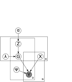
Figure 1: Graphical model.

2.1 Defining a distribution over infinite binary matrices

We now define our infinite model by taking the limit of a series of finite models.

Start with a finite model

We derive the distribution on $\mathbf{Z}$ by defining a finite $K$ model and taking the limit as $K\rightarrow\infty$. We then show how the infinite case corresponds to a simple stochastic process.

We have $D$ dimensions and $K$ hidden sources. Recall that $z_{dk}$ of matrix $\mathbf{Z}$ tells us whether hidden source $k$ contributes to dimension $d$. We assume that the probability of a source $k$ contributing to any dimension is $\pi_{k}$, and that the rows are generated independently. We find

$$P(\mathbf{Z}|\bolds{\pi})=\prod_{k=1}^{K}\prod_{d=1}^{D}P(z_{dk}|\pi_{k})=\prod_{k=1}^{K}\pi_{k}^{m_{k}}(1-\pi_{k})^{D-m_{k}},$$ (3)

where $m_{k}=\sum_{d=1}^{D}z_{dk}$ is the number of dimensions to which source $k$ contributes. The inner term of the product is a binomial distribution, so we choose the conjugate Beta$(r,s)$ distribution for $\pi_{k}$. For now we take $r=\frac{\alpha}{K}$ and $s=1$, where $\alpha$ is the strength parameter of the IBP. The model is defined by

$$\pi_{k}|\alpha \sim \operatorname{Beta}\biggl{(}\frac{\alpha}{K},1\biggr{)},$$ (4)

$$z_{dk}|\pi_{k} \sim \operatorname{Bernoulli}(\pi_{k}).$$ (5)

Due to the conjugacy between the binomial and beta distributions, we are able to integrate out $\pi$ to find

$$P(\mathbf{Z})=\prod_{k=1}^{K}\frac{(\alpha/K)\Gamma(m_{k}+{\alpha}/{K})\Gamma(D-m_{k}+1)}{\Gamma(D+1+{\alpha}/{K})},$$ (6)

where $\Gamma(\cdot)$ is the Gamma function.

Take the infinite limit

Griffiths and Ghahramani (2006) define a scheme to order the nonzero rows of $\mathbf{Z}$ which allows us to take the limit $K\rightarrow\infty$ and find

$$P(\mathbf{Z})=\frac{\alpha^{K_{+}}}{\prod_{h>0}K_{h}!}\exp{(-\alpha H_{D})}\prod_{k=1}^{K_{+}}\frac{(D-m_{k})!(m_{k}-1)!}{N!},$$ (7)

where $K_{+}$ is the number of active features (i.e., nonzero columns of $\mathbf{Z}$), $H_{D}=\sum_{j=1}^{D}\frac{1}{j}$ is the $D$th harmonic number, and $K_{h}$ is the number of rows whose entries correspond to the binary number $h$.

Go to an Indian Buffet

This distribution corresponds to a simple stochastic process, the Indian Buffet Process. Consider a buffet with a seemingly infinite number of dishes (hidden sources) arranged in a line. The first customer (observed dimension) starts at the left and samples $\operatorname{Poisson}(\alpha)$ dishes. The $i$th customer moves from left to right sampling dishes with probability $\frac{m_{k}}{i}$ where $m_{k}$ is the number of customers to have previously sampled dish $k$. Having reached the end of the previously sampled dishes, he tries $\operatorname{Poisson}(\frac{\alpha}{i})$ new dishes. Figure 2 shows two draws from the IBP for two different values of $\alpha$.

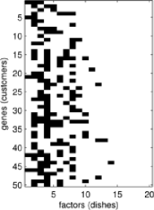
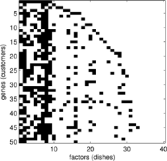
(a)	(b)

Figure 2: Draws from the one parameter IBP for two different values of $\alpha$. (a) $\alpha=4$. (b) $\alpha=8$.

If we apply the same ordering scheme to the matrix generated by this process as for the finite model, we recover the correct exchangeable distribution. Since the distribution is exchangeable with respect to the customers, we find by considering the last customer that

$$P(z_{kt}=1|\mathbf{z}_{-kn})=\frac{m_{k,-t}}{D},$$ (8)

where $m_{k,-t}=\sum_{s\neq t}z_{ks}$, which is used in sampling $\mathbf{Z}$. By exchangeability and considering the first customer, the number of active sources for each dimension follows a Poisson$(\alpha)$ distribution, and the expected number of entries in $\mathbf{Z}$ is $D\alpha$. We also see that the number of active features $K_{+}=\sum^{D}_{d=1}\operatorname{Poisson}(\frac{\alpha}{d})=\operatorname{Poisson}(\alpha H_{D})$.

3 Related work

The Bayesian Factor Regression Model (BFRM) of West et al. (2007) is closely related to the finite version of our model. The key difference is the use of a hierarchical sparsity prior. Each element of $\mathbf{G}$ has prior of the form

$$g_{dk}\sim(1-\pi_{dk})\delta_{0}(g_{dk})+\pi_{dk}\mathcal{N}(g_{dk};0,\lambda_{k}^{-1}).$$

The finite IBP model is equivalent to setting $\pi_{dk}=\pi_{k}\sim\operatorname{Beta}(\alpha/K,1)$ and then integrating out $\pi_{k}$. In BFRM a hierarchical prior is used:

$$\pi_{dk}\sim(1-\rho_{k})\delta_{0}(\pi_{dk})+\rho_{k}\operatorname{Beta}\bigl{(}\pi_{dk};am,a(1-m)\bigr{)},$$

where $\rho_{k}\sim\operatorname{Beta}(sr,s(1-r))$. Nonzero elements of $\pi_{dk}$ are given a diffuse prior favoring larger probabilities [$a=10$, $m=0.75$ are suggested in West et al. (2007)], and $\rho_{k}$ is given a prior which strongly favors small values, corresponding to a sparse solution (e.g., $s=D$, $r=\frac{5}{D}$).

Note that on integrating out $\pi_{dk}$, the prior on $g_{dk}$ is

$$g_{dk}\sim(1-m\rho_{k})\delta_{0}(g_{dk})+m\rho_{k}\mathcal{N}(g_{dk};0,\lambda_{k}^{-1}).$$

This hierarchical sparsity prior is motivated by improved interpretability in terms of less uncertainty in the posterior as to whether an element of $G$ is nonzero. However, this comes at a cost of significantly increased computation and reduced predictive performance, suggesting that the uncertainty removed from the posterior was actually important.

The LASSO-based Sparse PCA (SPCA) method of Zou, Hastie and Tibshirani (2004) and Witten, Tibshirani and Hastie (2009) has similar aims to our work in terms of providing a sparse variant of PCA to aid interpretation of the results. However, since SPCA is not formulated as a generative model, it is not necessarily clear how to choose the regularization parameters or dimensionality without resorting to cross-validation. In our experimental comparison to SPCA, we adjust the regularization constants such that each component explains roughly the same proportion of the total variance as the corresponding standard (nonsparse) principal component.

4 Inference

Given the observed data $\mathbf{Y}$, we wish to infer the hidden sources $\mathbf{X}$, which sources are active $\mathbf{Z}$, the mixing matrix $\mathbf{G}$, and all hyperparameters. We use Gibbs sampling, but with Metropolis–Hastings (MH) steps for sampling new features. We draw samples from the marginal distribution of the model parameters given the data by successively sampling the conditional distributions of each parameter in turn, given all other parameters.

Since we assume independent Gaussian noise, the likelihood function is

$$P(\mathbf{Y}|\mathbf{G},\mathbf{X},\bolds{\psi}) = \prod_{n=1}^{N}\frac{1}{(2\pi)^{D/2}|\bolds{\psi}|^{1/2}}$$

$${}\times\exp\biggl{(}-\frac{1}{2}(\mathbf{y}_{n}-\mathbf{G}\mathbf{x}_{n})^{T}\bolds{\psi}^{-1}(\mathbf{y}_{n}-\mathbf{G}\mathbf{x}_{n})\biggr{)},$$

where $\bolds{\psi}$ is a diagonal noise covariance matrix.

Notation

We use $-$ to denote the “rest” of the model, that is, the values of all variables not explicitly conditioned upon in the current state of the Markov chain. The $r$th row and $c$th column of matrix $A$ are denoted $A_{r:}$ and $A_{:c}$ respectively.

Mixture coefficients

We first derive a Gibbs sampling step for an individual element of the IBP matrix, $Z_{dk}$, determining whether factor $k$ is active for dimension $d$. Recall that $\lambda_{k}$ is the precision (inverse covariance) of the factor loadings for the $k$th factor. The ratio of likelihoods can be calculated using equation (4). Integrating out the $(d,k)$th element of the factor loading matrix $g_{dk}$ [whose prior is given by equation (2)], we obtain

$$\frac{P(\mathbf{Y}|Z_{dk}=1,-)}{P(\mathbf{Y}|Z_{dk}=0,-)} = \frac{\int P(\mathbf{Y}|g_{dk},-)\mathcal{N}(g_{dk};0,\lambda^{-1}_{k})\,dg_{dk}}{P(\mathbf{Y}|g_{dk}=0,-)}$$ (10)

$$= \sqrt{\frac{\lambda_{k}}{\lambda}}\exp\biggl{(}\frac{1}{2}\lambda\mu^{2}\biggr{)},$$ (11)

where we have defined $\lambda=\psi^{-1}_{d}X_{k:}^{T}X_{k:}+\lambda_{k}$ and $\mu=\frac{\psi^{-1}_{d}}{\lambda}X_{k:}^{T}\hat{E}_{d:}$ with the matrix of residuals $\hat{\mathbf{E}}=\mathbf{Y}-\mathbf{G}\mathbf{X}$ evaluated with $g_{dk}=0$. The dominant calculation is that for $\mu$ since the calculation for $\lambda$ can be cached. This operation is $O(N)$ and must be calculated $D\times K$ times, so sampling the IBP matrix, $\mathbf{Z}$, and factor loading matrix, $\mathbf{G}$, is order $O(NDK)$.

From the exchangeability of the IBP, we can imagine that dimension $d$ was the last to be observed, so that the ratio of the priors is

$$\frac{P(Z_{dk}=1|-)}{P(Z_{dk}=0|-)}=\frac{m_{-d,k}}{N-1-m_{-d,k}},$$ (12)

where $m_{-d,k}$ is the number of dimensions for which factor $k$ is active, excluding the current dimension $d$. Multiplying equations (11) and (12) gives the expression for the ratio of posterior probabilities for $Z_{dk}$ being 1 or 0, which is used for sampling. If $Z_{dk}$ is set to 1, we sample $g_{dk}|-\sim\mathcal{N}(\mu,\lambda^{-1})$ with $\mu,\lambda$ defined as for equation (11).

Adding new features

$\mathbf{Z}$ is a matrix with infinitely many columns, but the nonzero columns contribute to the likelihood and are held in memory. However, the zero columns still need to be taken into account since the number of active factors can change. Let $\kappa_{d}$ be the number of columns of $\mathbf{Z}$ which contain 1 only in row $d$, that is, the number of features which are active only for dimension $d$. Note that due to the form of the prior for elements of $\mathbf{Z}$ given in equation (12), $\kappa_{d}=0$ for all $d$ after a sampling sweep of $\mathbf{Z}$. Figure 3 illustrates $\kappa_{d}$ for a sample $\mathbf{Z}$ matrix.

Figure 3: A diagram to illustrate the definition of $\kappa_{d}$, for $d=10$.

New features are proposed by sampling $\kappa_{d}$ with a MH step. It is possible to integrate out either the new elements of the mixing matrix, $\mathbf{g}$ (a $1\times\kappa_{d}$ vector), or the new rows of the latent feature matrix, $\mathbf{X}^{\prime}$ (a $\kappa_{d}\times N$ matrix), but not both. Since the latter generally has higher dimension, we choose to integrate out $\mathbf{X}^{\prime}$ and include $\mathbf{g}^{T}$ as part of the proposal. Thus, the proposal is $\xi=\{\kappa_{d},\mathbf{g}\}$, and we propose a move $\xi\rightarrow\xi^{*}$ with probability $J(\xi^{*}|\xi)$. In this case $\xi=\varnothing$ since, as noted above, $\kappa_{d}=0$ initially. The simplest proposal, following Meeds et al. (2006), would be to use the prior on $\xi^{*}$, that is,

$$J(\xi)=P(\kappa_{d}|\alpha)\cdot p(\mathbf{g}|\kappa_{d},\lambda_{k})=\operatorname{Poisson}(\kappa_{d};\gamma)\cdot N(\mathbf{g};0,\lambda_{k}^{-1}),$$

where $\gamma=\frac{\alpha}{D-1}$.

Unfortunately, the rate constant of the Poisson prior tends to be so small that new features are very rarely proposed, resulting in slow mixing. To remedy this, we modify the proposal distribution for $\kappa_{d}$ and introduce two tunable parameters, $\pi$ and $\lambda$:

$$J(\kappa_{d})=(1-\pi)\operatorname{Poisson}(\kappa_{d};\lambda\gamma)+\pi\mathbf{1}(\kappa_{d}=1).$$ (13)

Thus, the Poisson rate is multiplied by a factor $\lambda$, and a spike at $\kappa_{d}=1$ is added with mass $\pi$. The proposal is accepted with probability $\min{(1,a_{\xi\rightarrow\xi^{*}})}$ where

$$a_{\xi\rightarrow\xi^{*}} = \frac{P(\xi^{*}|-,Y)J(\xi|\xi^{*})}{P(\xi|-,Y)J(\xi^{*}|\xi)}$$

$$= \frac{P(Y|\xi^{*},-)P(\kappa_{d}|\alpha)p(\mathbf{g}|\kappa_{d},\lambda_{k})}{P(Y|-)J(\kappa_{d})p(\mathbf{g}|\kappa_{d},\lambda_{k})}=a_{l}\cdot a_{p},$$

where

$$a_{l} = \frac{P(Y|\xi^{*},-)}{P(Y|-)},$$ (15)

$$a_{p} = \frac{P(\kappa_{d}|\alpha)}{J(\kappa_{d})}=\frac{\operatorname{Poisson}(\kappa_{d};\gamma)}{\operatorname{Poisson}(\kappa_{d};\lambda\gamma)}.$$ (16)

Note that we take $J(\xi|\xi^{*})=1$ since $\xi=\varnothing$. To calculate the likelihood ratio, $a_{l}$, we need the collapsed likelihood under the new proposal:

$$P(Y_{d:}|\xi^{*},-) = \prod_{n=1}^{N}\int P(Y_{dn}|\xi^{*},\mathbf{x}^{\prime}_{n},-)P(\mathbf{x}^{\prime}_{n})\,d\mathbf{x}^{\prime}$$

$$= \prod_{n=1}^{N}(2\pi\psi_{d}^{-1})^{-{1/2}}(2\pi)^{\kappa_{d}/2}|\mathbf{M}|^{-{1/2}}$$

$${}\times\exp\biggl{(}\frac{1}{2}(\mathbf{m}_{n}^{T}\mathbf{M}\mathbf{m}_{n}-\psi_{d}^{-1}\hat{E}^{2}_{dn})\biggr{)},$$

where we have defined $\mathbf{M}=\psi_{d}^{-1}\mathbf{g}\mathbf{g}^{T}+I_{\kappa_{d}}$ and $\mathbf{m}_{n}=\mathbf{M}^{-1}\psi_{d}^{-1}\mathbf{g}\hat{E}_{dn}$ with the matrix of residuals $\hat{\mathbf{E}}=\mathbf{Y}-\mathbf{G}\mathbf{X}$. The likelihood under the current sample is

$$P(Y_{d:}|\xi,-)=\prod_{n=1}^{N}(2\pi\psi_{d}^{-1})^{-{1/2}}\exp\biggl{(}-\frac{1}{2}\psi_{d}^{-1}\hat{E}^{2}_{dn}\biggr{)}.$$ (19)

Substituting these likelihood terms into the expression for the ratio of likelihood terms, $a_{l}$, gives

$$a_{l}=(2\pi)^{N\kappa_{d}/2}|\mathbf{M}|^{-{N/2}}\exp\biggl{(}\frac{1}{2}\sum_{n}\mathbf{m}_{n}^{T}\mathbf{M}\mathbf{m}_{n}\biggr{)}.$$ (20)

We found that appropriate scheduling of the sampler improved mixing, particularly with respect to adding new features. The final scheme we settled on is described in Algorithm 1.

Algorithm 1 One iteration of the NSFA sampler

  for $d=1$ to $D$ do

     for $k=1$ to $K$ do

        Sample $Z_{dk}$

     end for

     Sample $\kappa_{d}$

  end for

  for $n=1$ to $N$ do

     Sample $X_{:n}$

  end for

  Sample $\alpha,\phi,\lambda_{g}$

IBP parameters

We can choose to sample the IBP strength parameter $\alpha$, with conjugate $\operatorname{Gamma}(e,f)$ prior (note that we use the inverse scale parameterization of the Gamma distribution). The conditional prior of equation (7) acts as the likelihood term and the posterior update is as follows:

$$P(\alpha|\mathbf{Z})\propto P(\mathbf{Z}|\alpha)P(\alpha)=\operatorname{Gamma}(\alpha;K_{+}+e,f+H_{D}),$$ (21)

where $K_{+}$ is the number of active sources and $H_{D}=\sum_{j=1}^{D}\frac{1}{j}$ is the $D$th harmonic number.

The remaining sampling steps are standard, but are included here for completeness.

Latent variables

Sampling the columns $\mathbf{x}_{n}$ of the latent variable matrix $\mathbf{X}$ for each $t\in[1,\dots,N]$, we have

$$P(\mathbf{x}_{n}|-)\propto P(\mathbf{y}_{n}|\mathbf{x}_{n},-)P(\mathbf{x}_{n})=\mathcal{N}(\mathbf{x}_{n};\bolds{\mu}_{n},\bolds{\Lambda}),$$ (22)

where we have defined $\bolds{\Lambda}=\mathbf{G}^{T}\bolds{\psi}^{-1}\mathbf{G}+I$ and $\bolds{\mu}_{n}=\bolds{\Lambda}^{-1}\mathbf{G}^{T}\bolds{\psi}^{-1}\mathbf{y}_{n}$. Note that since $\bolds{\Lambda}$ does not depend on $n$, we only need to compute and invert it once per iteration. Calculating $\bolds{\Lambda}$ is order $O(K^{2}D)$, and inverting it is $O(K^{3})$. Calculating $\bolds{\mu}_{t}$ is order $O(KD)$ and must be calculated for all $N$ $\mathbf{x}_{t}$’s, a total of $O(NKD)$. Thus, sampling $\mathbf{X}$ is order $O(K^{2}+K^{3}+NKD)$.

Factor precision

If the mixture coefficient prior precisions $\lambda_{k}$ are constrained to be equal, we have $\lambda_{k}=\lambda\sim\operatorname{Gamma}(c,d)$. The posterior update is then given by $\lambda|G\sim\operatorname{Gamma}(c+\frac{\sum_{k}m_{k}}{2},d+\sum_{d,k}G^{2}_{dk})$.

However, if the variances are allowed to be different for each column of $\mathbf{G}$, we set $\lambda_{k}\sim\operatorname{Gamma}(c,d)$, and the posterior update is given by $\lambda_{k}|G\sim\operatorname{Gamma}(c+\frac{m_{k}}{2},d+\sum_{d}G^{2}_{dk})$. In this case we may also wish to share power across factors, in which case we also sample $d$. Putting a Gamma prior on $d$ such that $d\sim\operatorname{Gamma}(c_{0},d_{0})$, the posterior update is $d|\lambda_{k}\sim\operatorname{Gamma}(c_{0}+cK,d_{0}+\sum_{k=1}^{K}\lambda_{k})$.

Noise variance

The additive Gaussian noise can be constrained to be isotropic, in which case the inverse variance is given a Gamma prior: $\psi_{d}^{-1}=\psi^{-1}\sim\operatorname{Gamma}(a,b)$ which gives the posterior update $\psi^{-1}|-\sim\operatorname{Gamma}(a+\frac{ND}{2},b+\sum_{d,n}\hat{E}^{2}_{dn})$.

However, if the noise is only assumed to be independent (which we have found to be more appropriate for gene expression data), then each dimension has a separate noise variance, whose inverse is given a Gamma prior: $\psi_{d}^{-1}\sim\operatorname{Gamma}(a,b)$ which gives the posterior update $\psi_{d}^{-1}|-\sim\operatorname{Gamma}(a+\frac{N}{2},b+\sum_{n}E^{2}_{dn})$ where the matrix of residuals $\hat{\mathbf{E}}=\mathbf{Y}-\mathbf{G}\mathbf{X}$. We can share power between dimensions by giving the hyperparameter $b$ a hyperprior $\operatorname{Gamma}(a_{0},b_{0})$ resulting in the Gibbs update $b|-\sim\operatorname{Gamma}(a_{0}+aD,b_{0}+\sum_{d=1}^{D}\psi_{d}^{-1})$. This hierarchical prior results in soft coupling between the noise variances in each dimension, so we will refer to this variant as sc.

5 Results

We compare the following models:

• FA—Bayesian Factor Analysis; see, for example, Kaufman and Press (1973) or Rowe and Press (1998).

• AFA—Factor Analysis with ARD prior to determine active sources.

• FOK—The sparse Factor Analysis method of Fokoue (2004), Fevotte and Godsill (2006) and Archambeau and Bach (2009).

• SPCA—The Sparse PCA method of Zou, Hastie and Tibshirani (2004).

• BFRM—Bayesian Factor Regression Model of West et al. (2007).

• SFA—Sparse Factor Analysis, using the finite IBP.

• NSFA—The proposed model: Nonparametric Sparse Factor Analysis.

Note that all of these models can be learned using the software package we provide simply by using appropriate settings.

5.1 Synthetic data

Since generating a connectivity matrix $\mathbf{Z}$ from the IBP itself would clearly bias toward our model, we instead use the $D=100$ gene by $K=16$ factor E. Coli connectivity matrix derived in Kao et al. (2004) from RegulonDB and current literature. We ignore whether the connection is believed to be up or down regulation, resulting in a binary matrix $\mathbf{Z}$. We generate random data sets with $N=100$ samples by drawing the nonzero elements of $\mathbf{G}$ (corresponding to the elements of $\mathbf{Z}$ which are nonzero), and all elements of $\mathbf{X}$, from a zero mean unit variance Gaussian, calculating ${\mathbf{Y}=\mathbf{G}\mathbf{X}+\mathbf{E}}$, where $\mathbf{E}$ is Gaussian white noise with variance set to give a signal to noise ratio of 10.

Here we will define the reconstruction error $E_{r}$ as

$$E_{r}(G,\hat{G})=\frac{1}{DK}\sum_{k=1}^{K}\min_{\hat{k}\in\{1,\ldots,\hat{K}\}}\sum_{d=1}^{D}(G_{dk}-G_{d\hat{k}})^{2},$$

where $\hat{G},\hat{K}$ are the inferred quantities. Although we minimize over permutations, we do not minimize over rotations since, as noted in Fokoue (2004), the sparsity of the prior stops the solution being rotation invariant. We average this error over the last ten samples of the MCMC run. This error function does not penalize inferring extra spurious factors, so we will investigate this possibility separately. The precision and recall of active elements of the $\mathbf{Z}$ achieved by each algorithm (after thresholding for the nonsparse algorithms) are presented in the Supplementary Material, but omitted here since the results are consistent with the reconstruction error.

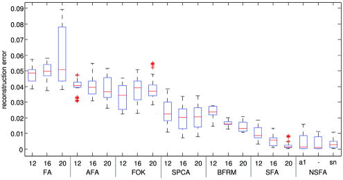
Figure 4: Boxplot of reconstruction errors for simulated data derived from the E. Coli connectivity matrix of Kao et al. (2004). Ten data sets were generated and the reconstruction error calculated for the last ten samples from each algorithm. Numbers refer to the number of latent factors used, $K$. a1 denotes fixing $\alpha=1$. sn denotes sharing power between noise dimensions.

The reconstruction error for each method with different numbers of latent features is shown in Figure 4. Ten random data sets were used and for the sampling methods (all but SPCA) the results were averaged over the last ten samples out of 1000. Unsurprisingly, plain Factor Analysis (FA) performs the worst, with increasing overfitting as the number of factors is increased. For $\hat{K}=20$ the variance is also very high, since the four spurious features fit noise. Using an ARD prior on the features (AFA) improves the performance, and overfitting no longer occurs. The reconstruction error is actually less for $\hat{K}=20$, but this is an artifact due to the reconstruction error not penalizing additional spurious features in the inferred $\mathbf{G}$. The Sparse PCA (SPCA) of Zou, Hastie and Tibshirani (2004) shows improved reconstruction compared to the nonsparse methods (FA and AFA), but does not perform as well as the Bayesian sparse models. Sparse factor analysis (SFA), the finite version of the full infinite model, performs very well. The Bayesian Factor Regression Model (BFRM) performs significantly better than the ARD factor analysis (AFA), but not as well as our sparse model (SFA). It is interesting that for BFRM the reconstruction error decreases significantly with increasing $\hat{K}$, suggesting that the default priors may actually encourage too much sparsity for this data set. Fokoue’s method (FOK) only performs marginally better than AFA, suggesting that this “soft” sparsity scheme is not as effective at finding the underlying sparsity in the data. Overfitting is also seen, with the error increasing with $\hat{K}$. This could potentially be resolved by placing an appropriate per factor ARD-like prior over the scale parameters of the Gamma distributions controlling the precision of elements of $\mathbf{G}$. Finally, the Nonparametric Sparse Factor Analysis (NSFA) proposed here and in Rai and Daumé III (2008) performs very well. With fixed $\alpha=1$ (a1) or inferring $\alpha$, we see very similar performance. Using the soft coupling (sc) variant which shares power between dimensions when fitting the noise variances seems to reduce the variance of the sampler, which is reasonable in this example since the noise was in fact isotropic.

Since the reconstruction error does not penalize spurious factors, it is important to check that NSFA is not scoring well simply by inferring many additional factors. Histograms for the number of latent features inferred for the nonparametric sparse model are shown in Figure 5. This represents an approximate posterior over $K$. For fixed $\alpha=1$ the distribution is centered around the true value of $K=16$, with minimal bias ($\mathbb{E}K=16.1$). The variance is significant (standard deviation of 1.46), but is reasonable considering the noise level ($\mathrm{SNR}=10$) and that in some of the random data sets, elements of $\mathbf{Z}$ which are 1 could be masked by very small corresponding values of $\mathbf{G}$. This hypothesis is supported by the results of a similar experiment where $\mathbf{G}$ was set equal to $\mathbf{Z}$. In this case, the sampler always converged to at least 16 features, but would also sometimes infer spurious features from noise (results not shown). When inferring $\alpha$ some bias and skew are noticeable. The mean of the posterior is now at $18.3$ with standard deviation $2.0$, suggesting there is little to gain from sampling $\alpha$ in this data.

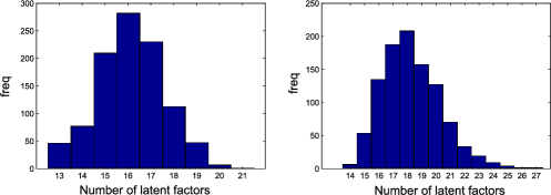
Figure 5: Histograms of the number of latent features inferred by the nonparametric sparse FA sampler for the last 100 samples out of 1000. Left: With $\alpha=1$. Right: Inferring $\alpha$.

5.2 Convergence

NSFA can suffer from slow convergence if the number of new features is drawn from the prior. Figure 6 shows how the different proposals for $\kappa_{d}$ effect how quickly the sampler reaches a sensible number of features. If we use the prior as the proposal distribution, mixing is very slow, taking around 5000 iterations to converge, as shown in Figure 6(a). If a mass of $0.1$ is added at $\kappa_{d}=1$ [see equation (13)], then the sampler reaches the equilibrium number of features in around 1500 iterations, as shown in Figure 6(b). However, if we try to add features even faster, for example, by setting the factor $\lambda=50$ in equation (13), then the sampling noise is greatly increased, as shown in Figure 6(c), and the computational cost also increases significantly because so many spurious features are proposed only to be rejected.

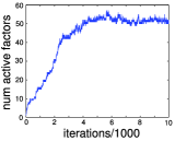
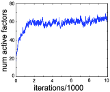
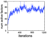
(a)	(b)	(c)

Figure 6: The effect of different proposal distributions for the number of new features. (a) Prior. (b) Prior plus $0.1\mathbb{I}(\kappa=1)$. (c) Factor $\lambda=50$.

5.3 Biological data: E. Coli time-series dataset

To assess the performance of each algorithm on the biological data where no ground truth is available, we calculated the test set log likelihood under the posterior. Ten percent of entries from $\mathbf{Y}$ were removed at random, ten times, to give ten data sets for inference. We do not use mean square error as a measure of predictive performance because of the large variation in the signal to noise ratio across gene expression level probes.

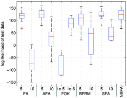
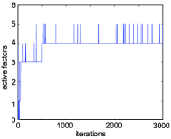
(a)	(b)

Figure 7: Results on E. Coli time-series data set from Kao et al. (2004) ($N=24$, $D=100$, 3000 MCMC iterations). (a) Log likelihood of test data under each model based on the last 100 MCMC samples. The boxplots show variation across 10 different random splits of the data into training and test sets. (b) Number of active latent features during a typical MCMC run of the NSFA model.

The test log likelihood achieved by the various algorithms on the E. Coli data set from Kao et al. (2004), including 100 genes at 24 time-points, is shown in Figure 7(a). On this simple data set incorporating sparsity doesn’t improve predictive performance. Overfitting the number of latent factors does damage performance, although using the ARD or sparse prior alleviates the problem. Based on predictive performance of the finite models, five is a sensible number of features for this data set: the NSFA model infers a median number of 4 features, with some probability of there being 5, as shown in Figure 7(b).

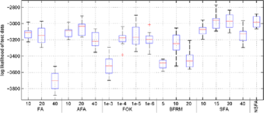
(a)

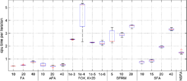
(b)

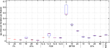
(c)

Figure 8: Results on breast cancer data set ($N=251$, $D=226$, 3000 MCMC iterations). (a) Predictive performance: log likelihood of test (the 10% missing) data under each model based on the last 100 MCMC samples. Higher values indicate better performance. The boxplots show variation across 10 different random splits of the data into training and test sets. (b) CPU time (in seconds) per iteration, averaged across the 3000 iteration run. (c) CPU time (in seconds) per iteration divided by the number of features at that iteration, averaged across all iterations.

5.4 Breast cancer data set

We assess these algorithms in terms of predictive performance on the breast cancer data set of West et al. (2007), including 226 genes across 251 individuals. We find that all the finite models are sensitive to the choice of the number of factors, $K$. The samplers were found to have converged after around 1000 samples according to standard multiple chain convergence measures, so 3000 MCMC iterations were used for all models. The predictive log likelihood was calculated using the final 100 MCMC samples. Figure 8(a) shows test set log likelihoods for 10 random divisions of the data into training and test sets. Factor analysis (FA) shows significant overfitting as the number of latent features is increased from 20 to 40. Using the ARD prior prevents this overfitting (AFA), giving improved performance when using 20 features and only slightly reduced performance when 40 features are used. The sparse finite model (SFA) shows an advantage over AFA in terms of predictive performance as long as underfitting does not occur: performance is comparable when using only 10 features. However, the performance of SFA is sensitive to the choice of the number of factors, $K$. The performance of the sparse nonparametric model (NSFA) is comparable to the sparse finite model when an appropriate number of features is chosen, but avoids the time consuming model selection process. Fokoue’s method (FOK) was run with $K=20$ and various settings of the hyperparameter $d$ which controls the overall sparsity of the solution. The model’s predictive performance depends strongly on the setting of this parameter, with results approaching the performance of the sparse models (SFA and NSFA) for $d=10^{-4}$. The performance of BFRM on this data set is noticeably worse than the other sparse models.

We now consider the computation cost of the algorithms. As described in Section 4, sampling $\mathbf{Z}$ and $\mathbf{G}$ takes order $O(NKD)$ operations per iteration, and sampling $\mathbf{X}$ takes $O(K^{2}+K^{3}+ND)$. However, for the moderate values encountered for data sets 1 and 2, the main computational cost is sampling the nonzero elements of $\mathbf{G}$, which takes $O((1-s)DK)$ where $s$ is the sparsity of the model. Figure 8(c) shows the mean CPU time per iteration divided by the number of features at that iteration. Naturally, straight FA is the fastest, taking only around $0.025s$ per iteration per feature. The value increases slightly with increasing $K$, suggesting that here the $O(K^{2}D+K^{3})$ calculation and inversion of $\bolds{\lambda}$, the precision of the conditional on $\mathbf{X}$, must be contributing. The computational cost of adding the ARD prior is negligible (AFA). The CPU time per iteration is just over double for the sparse finite model (SFA), but the cost actually decreases with increasing $K$, because the sparsity of the solution increases to avoid overfitting. There are fewer nonzero elements of $\mathbf{G}$ to sample per feature, so the CPU time per feature decreases. The CPU time per iteration per feature for the nonparametric sparse model (NSFA) is somewhat higher than for the finite model because of the cost of the feature birth and death process. However, Figure 8(b) shows the absolute CPU time per iteration, where we see that the nonparametric model is only marginally more expensive than the finite model of appropriate size $\hat{K}=15$ and cheaper than choosing an unnecessarily large finite model (SFA with $K=20$, 40). Fokoue’s method (FOK) has comparable computational performance to the sparse finite model, but interestingly has increased cost for the optimal setting of $d=10^{-4}$. The parameter space for FOK is continuous, making search easier but requiring a normal random variable for every element of $\mathbf{G}$. BFRM pays a considerable computational cost for both the hierarchical sparsity prior and the DP prior on $\mathbf{X}$. SPCA was not run on this data set, but results on the synthetic data in Section 5.1 suggest it is somewhat faster than the sampling methods, but not hugely so. The computational cost of SPCA is $ND^{2}+mO(D^{2}K+DK^{2}+D^{3})$ in the $N>D$ case (where $m$ is the number of iterations to convergence) and $ND^{2}+mO(D^{2}K+DK^{2})$ in the $D>N$ case, taking the limit $\lambda\rightarrow\infty$. In either case an individual iteration of SPCA is more expensive than one sampling iteration of NSFA (since $K<D$), but fewer iterations will generally be required to reach convergence of SPCA than are required to ensure mixing of NSFA.

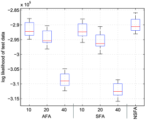
Figure 9: Test set log likelihoods on Prostate cancer data set from Yu et al. (2004), including 12557 genes across 171 individuals (1000 MCMC iterations).

5.5 Prostate cancer data set

Figure 9 shows the predictive performance of AFA, FOK and NSFA on the prostate cancer data set of Yu et al. (2004), for ten random splits into training and test data. The boxplots show variation from ten random splits into training and test data. The large number of genes ($D=12557$ across $N=171$ individuals) in this data set makes inference slower, but the problem is manageable since the computational complexity is linear in the number of genes. Despite the large number of genes, the appropriate number of latent factors, in terms of maximizing predictive performance, is still small, around 10 (NSFA infers a median of 12 factors). This may seem small relative to the number of genes, but it should be noted that the genes included in the breast cancer and E. Coli data sets are those capturing the most variability. Surprisingly, SFA actually performed slightly worse on this data set than AFA. Both are highly sensitive to the number of latent factors chosen. NSFA, however, gives better predictive log likelihoods than either finite model for any fixed number of latent factors $K$. Running 1000 iterations of NSFA on this data set takes under 8 hours. BFRM and FOK were impractically slow to run on this data set.

6 Discussion

We have seen that in both the E. Coli and breast cancer data sets that sparsity can improve predictive performance, as well as providing a more easily interpretable solution. Using the IBP to provide sparsity is straightforward, and allows the number of latent factors to be inferred within a well-defined theoretical framework. This has several advantages over manually choosing the number of latent factors. Choosing too few latent factors damages predictive performance, as seen for the breast cancer data set. Although choosing too many latent factors can be compensated for by using appropriate ARD-like priors, we find this is typically more computationally expensive than the birth and death process of the IBP. Manual model selection is an alternative but is time consuming. Finally, we show that running NSFA on full gene expression data sets with 10000$+$ genes is feasible so long as the number of latent factors remains relatively small. An interesting direction for this research is how to incorporate prior knowledge, for example, if certain transcription factors are known to regulate specific genes. Incorporating this knowledge could both improve the performance of the model and improve interpretability by associating latent variables with specific transcription factors. Another possibility is incorporating correlations in the Indian Buffet Process, which has been proposed for simpler models [Doshi-Velez and Ghahramani (2009); Courville, Eck and Bengio (2009)]. This would be appropriate in a gene expression setting where multiple transcription factors might be expected to share sets of regulated genes due to common motifs. Unfortunately, performing MCMC in all but the simplest of these models suffers from slow mixing.

References

- Archambeau and Bach (2009) {binproceedings}[author] \bauthor\bsnmArchambeau, \bfnmC.\binitsC. and \bauthor\bsnmBach, \bfnmF.\binitsF. (\byear2009). \btitleSparse probabilistic projections. In \bbooktitleProceedings of the Conference on Neural Information Processing Systems (NIPS) (\beditor\bfnmDaphne\binitsD. \bsnmKoller, \beditor\bfnmDale\binitsD. \bsnmSchuurmans, \beditor\bfnmYoshua\binitsY. \bsnmBengio and \beditor\bfnmLéon\binitsL. \bsnmBottou, eds.) \bpages73–80. \bpublisherMIT Press, \baddressCambridge, MA. \endbibitem
- Courville, Eck and Bengio (2009) {binproceedings}[author] \bauthor\bsnmCourville, \bfnmAaron C.\binitsA. C., \bauthor\bsnmEck, \bfnmDouglas\binitsD. and \bauthor\bsnmBengio, \bfnmYoshua\binitsY. (\byear2009). \btitleAn infinite factor model hierarchy via a noisy-or mechanism. In \bbooktitleAdvances in Neural Information Processing Systems \bvolume21. \bpublisherMIT Press, \baddressCambridge, MA. \endbibitem
- Doshi-Velez and Ghahramani (2009) {binproceedings}[author] \bauthor\bsnmDoshi-Velez, \bfnmFinale\binitsF. and \bauthor\bsnmGhahramani, \bfnmZoubin\binitsZ. (\byear2009). \btitleCorrelated non-parametric latent feature models. In \bbooktitleProceedings of the Twenty-Fifth Conference on Uncertainty in Artificial Intelligence \bpages143–150. \bpublisherAUAI Press, \baddressArlington, VA. \endbibitem
- Fevotte and Godsill (2006) {barticle}[author] \bauthor\bsnmFevotte, \bfnmC.\binitsC. and \bauthor\bsnmGodsill, \bfnmS. J.\binitsS. J. (\byear2006). \btitleA Bayesian approach for blind separation of sparse sources. \bjournalIEEE Transactions on Audio, Speech, and Language Processing \bvolume14 \bpages2174–2188. \endbibitem
- Fokoue (2004) {btechreport}[author] \bauthor\bsnmFokoue, \bfnmE\binitsE. (\byear2004). \btitleStochastic determination of the intrinsic structure in Bayesian factor analysis. \btypeTechnical Report No. \bnumber17, \binstitutionStatistical and Applied Mathematical Sciences Institute. \endbibitem