Abstract

We use molecular dynamics (MD) to study the kinetics of surface enrichment (SE) in a stable homogeneous mixture ($AB$), placed in contact with a surface which preferentially attracts $A$. The SE profiles show a characteristic double-exponential behavior with two length scales: $\xi_{-}$, which rapidly saturates to its equilibrium value, and $\xi_{+}$, which diverges as a power-law with time ($\xi_{+}\sim t^{\theta}$). We find that hydrodynamic effects result in a crossover of the growth exponent from $\theta\simeq 0.5$ to $\theta\simeq 1.0$. There is also a corresponding crossover in the growth dynamics of the SE-layer thickness.

1 Introduction

There is a wide range of physical phenomena associated with binary ($AB$) mixtures in contact with a surface ($S$). Typically, the surface has a preferential attraction for one of the components of the mixture (say, $A$). A rich phase diagram arises, depending on the interactions between $AB,AS,BS$ and the temperature $T$ [1, 2, 3, 4, 5]. For simplicity, we focus on a semi-infinite geometry. If the bulk system is below the miscibility gap, the $AB$ interface meets the surface at a contact angle $\theta$, which is determined by Young’s equation [6]:

$$\gamma_{AB}\,\mathrm{cos}\theta=\gamma_{BS}-\gamma_{AS},$$ (1)

where $\gamma_{\alpha\beta}$ denotes the surface tension between $\alpha$ and $\beta$. For $\gamma_{AB}>\gamma_{BS}-\gamma_{AS}$, the surface undergoes partial wetting. For $\gamma_{AB}<\gamma_{BS}-\gamma_{AS}$, Young’s equation does not have a solution and the surface is completely wet in equilibrium, i.e., the $B$-rich phase is expelled from the surface. On the other hand, if the bulk system is above the miscibility gap, there will be no macroscopic phase separation. Nevertheless, the surface is enriched in the preferred component – the degree of enrichment depends upon various interaction strengths. Both the problems of wetting and surface enrichment are of great scientific and technological importance.

We have a long-standing interest in the kinetics of mixtures at surfaces. Again, a rich set of problems arises in this context. Consider a homogeneous $AB$ mixture (at high temperatures, $T=\infty$) placed in contact with a flat surface (located at $z=0$) which prefers $A$. If the system is suddenly quenched below the miscibility gap at time $t=0$, it undergoes phase separation in the bulk [7, 8], and segregates into $A$-rich and $B$-rich domains. Simultaneously, the surface is wetted by $A$. The interplay of these two kinetic processes, i.e., phase separation and wetting, results in surface-directed spinodal decomposition (SDSD) waves which originate at the surface and propagate into the bulk. There has been intense experimental [9, 10, 11, 12] and theoretical [13, 14, 15] interest in SDSD. Alternatively, we can consider quenches to temperatures above the miscibility gap or to the metastable region of the phase diagram [16]. In this case, the mixture is stable and continues to be homogeneous for large $z$. However, the surface becomes enriched in the preferred component, resulting in a time-dependent surface-enrichment (SE) profile, which propagates into the bulk. This phenomenon of SE is well known in the context of polymer blends [17, 18, 19, 20, 21, 22] and biopolymer mixtures [23], binary alloys [24, 25], and the wetting of surfaces of fluids [4, 26].

In this paper, we undertake a comprehensive molecular dynamics (MD) study of the kinetics of SE. This paper has two primary goals. First, we would like to test the theoretical results for enrichment kinetics (summarized later) via a realistic microscopic MD simulation. The available numerical studies of this problem have focused on Langevin simulations of phenomenological models. Second, we would like to examine whether hydrodynamic effects (which are naturally incorporated in our MD simulations) have any effect on SE kinetics. After all, many experiments in this area involve fluid mixtures or polymer mixtures, where velocity fields play a significant role. In the context of phase-separation kinetics, we know that hydrodynamic effects drastically alter the late-stage dynamics – both without surfaces [8, 7, 27, 28, 29] and with surfaces [30, 31, 32].

This paper is organized as follows. Section 2 describes the details of our MD simulations. In Sec. 3, we present comprehensive numerical results and compare them with theoretical predictions. Finally, Sec. 4 concludes this paper with a summary and discussion.

2 Details of Molecular Dynamics Simulations

Following Das et al. [33], we consider a binary ($AB$) fluid mixture of point particles confined in a rectangular box of volume $V=L\times L\times D$. We apply periodic boundary conditions in the $x$ and $y$ directions, while impenetrable walls or surfaces are present at $z=0$ and $z=D$. These surfaces give rise to an integrated Lennard-Jones (LJ) potential ($\alpha=A,B$):

$$u_{w}(z)=\frac{2\pi n\sigma^{3}}{3}\left[\frac{2\epsilon_{r}}{15}{\left(\frac{\sigma}{z^{\prime}}\right)}^{9}-\delta_{\alpha}\epsilon_{a}{\left(\frac{\sigma}{z^{\prime}}\right)}^{3}\right],$$ (2)

where $n$ is the reference density of the fluid, and $\sigma$ is the LJ diameter of the particles. In Eq. (2), $\epsilon_{r}$ and $\epsilon_{a}$ are the strengths of the repulsive and attractive parts of the wall potentials. For the wall at $z=0$, we choose $\delta_{A}=1$ and $\delta_{B}=0$, so there is only a repulsion for $B$ particles, while $A$ particles are attracted at large distances and repelled at short distances. For the wall at $z=D$, we set $\delta_{A}=\delta_{B}=0$, so that both $A$ and $B$ particles feel only repulsion. Further, $z^{\prime}=z+\sigma/2$ for the wall at $z=0$, and $z^{\prime}=D+\sigma/2-z$ for the wall at $z=D$. Therefore, the singularities of $u_{w}(z)$ do not occur within the box range $0\leq z\leq D$, but rather at $z=-\sigma/2$ and $z=D+\sigma/2$, respectively.

The particles in the system interact with LJ potentials:

$$u(r_{ij})=4\epsilon_{\alpha\beta}\left[\left(\frac{\sigma}{r_{ij}}\right)^{12}-\left(\frac{\sigma}{r_{ij}}\right)^{6}\right],$$ (3)

where $r_{ij}=|\vec{r}_{i}-\vec{r}_{j}|$; $\alpha,\beta=A,B$. The energy scales are

$$\epsilon_{AA}=\epsilon_{BB}=2\epsilon_{AB}=\epsilon,$$ (4)

for which the equilibrium phase behavior is well studied [34, 35, 36]. We use the truncated, shifted and force-corrected LJ potential with $r_{ij}=r_{c}=2.5\sigma$ [37]. We consider the case with equal numbers of $A$ and $B$ particles ($N_{A}=N_{B}=N/2$), and their masses are set to be equal, $m_{A}=m_{B}=m=1$. We also set $\sigma=1$, $\epsilon=1$ and $k_{B}=1$, such that the MD time unit is

$$t_{0}={\left(\frac{m\sigma^{2}}{48\epsilon}\right)}^{1/2}=\frac{1}{\sqrt{48}}.$$ (5)

We work with a high-density liquid having $n=N/V=1$, which makes the system incompressible. Notice that crystallization is not a problem at the temperatures of interest. Finally, simulations were run for three surface energy strengths – $\epsilon_{a}=1.2,2.0,3.0$ with $\epsilon_{r}=0.5$.

For our study, we chose $L=32$ and $D=64$ ($N=66536$ particles). As the bulk remains homogeneous, the lateral size $L$ (in the $x,y$ directions) is not severely constrained. However, in the direction perpendicular to the surface located at $z=0$, we need sufficiently large $D$ to ensure decay of the enrichment profiles as $z\rightarrow D$. For the range of times studied here ($t\leq 7000$), test runs with other linear dimensions showed that $D=64$ is large enough to eliminate finite-size effects, within the limits of our statistical accuracy. For a smaller system size ($D=32$), we encounter finite-size effects by $t\simeq 3000$. The statistical quantities presented here were obtained as averages over 50 independent runs. The MD runs were carried out using the standard Verlet velocity algorithm [38], with a time-step $\Delta t=0.07$ in MD units given by Eq. (5), and the Nosé-Hoover thermostat [38]. We prepared the homogeneous initial state for a run by equilibrating the mixture of $N$ particles at high $T$, in the specified volume with periodic boundary conditions in all directions. At time $t=0$, the system is quenched to $T=2.0\simeq 1.41T_{c}~{}(T_{c}\simeq 1.423)$ [35, 36], and surfaces are introduced at $z=0,D$.

3 Theoretical Background and Numerical Results

We are interested in the time-dependent morphology which arises during SE. We characterize the morphology via laterally-averaged depth profiles and their various properties, e.g., surface value of order parameter, zero-crossings, moments, etc. Before proceeding, it is useful to summarize theoretical results in this context.

3.1 Theoretical Background

Jones et al. [18, 19] have studied the kinetics of SE for polymer mixtures, and found that the enrichment profiles are characterized by diffusive length scales. Numerical studies of this problem (with both short-ranged and long-ranged surface fields) have been conducted by Jiang and Ebner [39] using MC simulations, and Toral and Chakrabarti [40] via Langevin simulations. Binder and Frisch [41] studied SE in a linearized Ginzburg-Landau (GL) model with a delta-function (short-ranged) surface potential. Their GL model was derived by coarse-graining the Kawasaki spin-exchange kinetic Ising model in the presence of a surface. Their results are expected to be valid in the weak-field regime, where the concentration variations are sufficiently weak that nonlinear effects can be neglected. Puri and Frisch (PF) [42] have also studied the case with a short-ranged surface potential in the framework of a linear theory. They also undertook Langevin simulations of the corresponding GL model for both weak and strong surface fields. In the latter case, linear theory is no longer applicable as the order parameter value at the surface becomes appreciably large. PF demonstrated that the morphological features predicted by linear theory are also seen in the nonlinear regime. These results were extended to the case with an arbitrary surface potential $V(z)$ by Frisch et al. (FPN) [43]. Here, we briefly summarize the results of PF and FPN.

Let us first discuss the modeling of segregation kinetics at surfaces [14, 15]. The bulk order parameter satisfies the Cahn-Hilliard (CH) equation:

$$\frac{\partial}{\partial t}\phi(\vec{\rho},z,t)=-\nabla^{2}\Big{[}\mathrm{sgn}(T_{c}-T)\phi-\phi^{3}+\frac{1}{2}\nabla^{2}\phi-V(z)\Big{]},\quad z>0.$$ (6)

Here, all the quantities have been rescaled into dimensionless units [44]. The order parameter $\phi(\vec{r},t)\simeq n_{A}(\vec{r},t)-n_{B}(\vec{r},t)$, where $n_{\alpha}(\vec{r},t)$ denotes the density of species $\alpha$ at space-point $\vec{r}$ and time $t$. We have decomposed coordinates as $\vec{r}\equiv(\vec{\rho},z)$, where $\vec{\rho}$ and $z$ denote coordinates parallel and perpendicular to the surface located at $z=0$. The function $\textrm{sgn}(x)=1$ for $x>0$ and $-1$ for $x<0$. The surface potential $V(z)\,(<0)$ is chosen so that it enriches the surface in $A$.

Equation (6) must be supplemented by two boundary conditions at $z=0$, as it is a fourth-order partial differential equation. Since the surface value of the order parameter is not a conserved quantity, we assume a nonconserved relaxational kinetics with time-scale $\tau_{0}$ for this quantity at the surface:

$$\tau_{0}\frac{\partial}{\partial t}\phi(\vec{\rho},0,t)=h_{1}+g\phi(\vec{\rho},0,t)+\gamma\frac{\partial}{\partial z}\phi(\vec{\rho},z,t)\bigg{|}_{z=0}+\tilde{\gamma}\nabla_{\|}^{2}\phi(\vec{\rho},0,t),$$ (7)

where $h_{1}=-V(0)$, and $g,\gamma,\tilde{\gamma}$ are phenomenological parameters, which are related to the bulk correlation length [44]. Finally, we implement the no-flux boundary condition at the surface, which enforces order parameter conservation:

$$0=\dfrac{\partial}{\partial z}\left[\mathrm{sgn}(T_{c}-T)\phi-\phi^{3}+\frac{1}{2}\nabla^{2}\phi-V(z)\right]\bigg{|}_{z=0}.$$ (8)

Equations (6)-(8) describe both SDSD (when $T<T_{c}$) and SE (when $T>T_{c}$), as long as the dynamics is diffusive. This is appropriate for phase separation in solid mixtures or the early stages of segregation in polymer mixtures. However, most experiments involve fluid mixtures, where hydrodynamic effects play an important role in the intermediate and late stages of phase separation. At a phenomenological level, hydrodynamic effects can be incorporated via the Navier-Stokes equation for the velocity field – the resultant coupled equations are known as Model H [30, 45]. This must be supplemented by appropriate boundary conditions at the surfaces. Alternatively, one can consider microscopic models of fluid mixtures at a surface, which naturally incorporate the fluid velocity field. We adopt the latter strategy in this paper, and use MD simulations to study SE in fluid mixtures.

For reference, it is useful to summarize results for the diffusive case. We consider the model in Eqs. (6)-(8) for $T>T_{c}$, as we are interested in the kinetics of SE. In this case, the order parameter field remains homogeneous in the direction parallel to the surface, i.e., we can neglect the $\vec{\rho}\,$-dependence of the order parameter $\phi(\vec{\rho},z,t)\simeq\phi(z,t)$. FPN have solved the linearized version of this model, which is appropriate when $\phi$ is small and the $\phi^{3}$-term can be neglected in Eqs. (6) and (8). Seeing that the bulk remains homogeneous, there is a significant enhancement of $\phi$ only for $z\simeq 0$. Thus, the linearized model is valid for weak surface fields. In this case, the results of FPN are as follows.

The SE profiles have a double-exponential form [41]:

$$\phi(z,t)\simeq B_{-}(t)\,\mathrm{e}^{-z/\xi_{-}(t)}-B_{+}(t)\,\mathrm{e}^{-z/\xi_{+}(t)},$$ (9)

where the amplitudes $B_{-}(t),B_{+}(t)>0$. Notice that the conservation constraint dictates that $B_{-}\xi_{-}=B_{+}\xi_{+}$. The quantities $B_{-}(t)$ and $\xi_{-}(t)$ rapidly saturate to their equilibrium values which depend on the surface potential:

$$B_{-}(t) \simeq a_{1},$$

$$\xi_{-}(t) \simeq b_{1}.$$ (10)

The other length scale $\xi_{+}(t)$ grows diffusively with time, and $B_{+}(t)$ shows a corresponding decay:

$$B_{+}(t) \simeq a_{2}\,t^{-1/2},$$

$$\xi_{+}(t) \simeq b_{2}\,t^{1/2}.$$ (11)

The other properties of the enrichment profiles are obtained from Eq. (9). An experimentally important quantity is the time-dependence of $\phi(z=0,t)$, the value of the order parameter at the surface [20, 21, 22]:

$$\phi(0,t)\simeq a_{1}-a_{2}\,t^{-1/2}.$$ (12)

Thus, $\phi(0,t)$ saturates diffusively to its equilibrium value. The thickness of the enrichment layer is measured as the first zero of the double-exponential profile. This increases logarithmically with time:

$$Z_{0}(t) \simeq \frac{\xi_{+}\xi_{-}}{\xi_{+}-\xi_{-}}\ln\left(\frac{B_{-}}{B_{+}}\right)$$ (13)

$$\simeq \frac{\xi_{-}}{2}\ln\left(\frac{t}{\tau}\right),\quad\tau={\left(\frac{a_{2}}{a_{1}}\right)}^{2}.$$

Finally, consider the time-dependence of the profile moments:

$$\langle z^{m}\rangle=\int_{0}^{\infty}\mathrm{d}z\,z^{m}\phi(z,t)\simeq\frac{1}{m!}\left(B_{-}\xi_{-}^{m+1}-B_{+}\xi_{+}^{m+1}\right).$$ (14)

Therefore, the asymptotic ($t\rightarrow\infty$) behavior of $\langle z^{m}\rangle$ is $\langle z^{m}\rangle\sim t^{m/2}$.

These results apply for diffusive transport and are universal for a wide set of potentials. They have been obtained in the context of a linear theory, and there is a range of weak surface fields where the analytical results obtained from the linear model agree well with the numerical solution of the nonlinear Eqs. (6)-(8) [43]. As the field strength is increased, the validity of linear theory breaks down in the vicinity of the surface as the degree of enrichment becomes larger. Nevertheless, FPN demonstrated that the diffusive behavior of various profile characteristics is unaffected, even in the strongly nonlinear regime.

As stated earlier, we have undertaken MD simulations to examine whether hydrodynamic effects have any impact on the above phenomenology. Let us next present results from these simulations.

3.2 Numerical Results

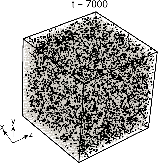
Figure 1: Snapshot of surface enrichment (SE) in a binary ($AB$) Lennard-Jones (LJ) mixture, which is confined in a box of size $L\times L\times D$ with $L=32$, $D=64$. (All lengths are measured in units of the LJ diameter.) Periodic boundary conditions are applied in the $x,y$ directions, while an impenetrable $L\times L$ surface at $z=0$ attracts the $A$-particles. For clarity, we show only part of the simulation box with $z\in[0,32]$. The initial condition for this run consisted of a random mixture of equal amounts of $A$ and $B$ particles ($N_{A}=N_{B}=32768$). Time is measured in dimensionless LJ units. For further details of the MD simulation, see Sec. 2. The $A$-particles are marked gray, and the $B$-particles are marked black. The snapshot corresponds to $t=7000$ for the surface potential in Eq. (2) with $\epsilon_{a}=3.0,\epsilon_{r}=0.5$. The $A$-rich enrichment layer is formed at $z=0$, while for large $z$, the stable mixture continues to be homogeneous.

Figure 1 shows a three-dimensional snapshot of SE in a binary ($AB$) mixture at $t=7000$. The surface field strengths are $\epsilon_{a}=3.0$ and $\epsilon_{r}=0.5$ in Eq. (2). We see the formation of an $A$-rich (marked in gray) layer at the surface ($z=0$), resulting in a time-dependent SE profile which propagates into the bulk. However, in the bulk (large $z$), the thermodynamically stable mixture continues to be homogeneous. In Fig. 2, we show cross-sections of the snapshots at $z=0$ for $t=70,7000$. The cross-section shows all $A$ atoms (marked gray) and all $B$ atoms (marked black) lying in the interval $z\in[0,\sigma]$.

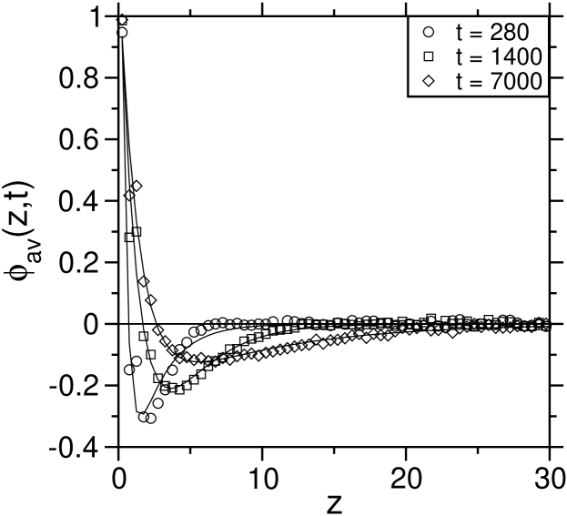
Figure 3: Laterally-averaged order parameter profiles [$\phi_{\textrm{av}}(z,t)$ vs. $z$] at the dimensionless times $t=280,1400,7000$. The surface potential is given by Eq. (2) with $\epsilon_{a}=2.0,\,\epsilon_{r}=0.5$. The double-exponential fits for the SE profiles are shown as solid lines.

In Fig. 3, we show the temporal evolution of the laterally-averaged order parameter profiles $\phi_{\mathrm{av}}(z,t)$ vs. $z$, obtained from our MD simulations [44]. The order parameter is defined in terms of the local densities as $\phi(\vec{r},t)=(n_{A}-n_{B})/(n_{A}+n_{B})$. The quantity $\phi_{\textrm{av}}(z,t)$ is obtained by averaging $\phi(\vec{r},t)$ in the directions parallel to the surface, and then further averaging over 50 independent runs. These laterally-averaged profiles are analogous to depth profiles measured in experiments – see Fig. 7 in Ref. [20] or Fig. 4 in Ref. [22]. The enrichment profiles are shown for the case with field strength $\epsilon_{a}=2.0$ at times $t=280,1400,7000$. It is clear that a layer rich in $A$ forms at the surface immediately after the field is turned on. Due to the conservation of the order parameter, there must be a corresponding depletion layer which decays to $\phi_{\textrm{av}}\simeq 0$ in the bulk. These profiles are in agreement with the experimental observations of Jones et al. [18] on blends of deuterated and protonated polystyrene, and the experimental results of Mouritsen [23] on biopolymer mixtures. Notice that similar profiles are seen for SDSD or surface-directed phase separation if the system is quenched to the metastable region of the phase diagram [16]. The evolution dynamics in that case is analogous to the SE problem as long as droplets are not nucleated in the system.

We make the following observations about the enrichment profiles in Fig. 3. First, for the field strengths we consider, the surface is strongly enriched in $A$: $\phi_{\textrm{av}}(0,t)\simeq 1$ for $\epsilon_{a}=2.0,3.0$. Thus, the linear theory is not applicable in the enrichment layer as this would require $\phi^{3}\ll\phi$. Second, at late times (say $t=7000$ in Fig. 3), the depletion region stretches deep into the bulk. To avoid finite-size effects, we confine our simulation to time regimes where the thickness of the depletion region $\ll D=64$, the box size in the $z$-direction. As shown in Fig. 3, the profiles are fitted very well by the superposition of two exponential functions as in Eq. (9). Our simulations show that $B_{-}(t)$ and $\xi_{-}(t)$ rapidly saturate to their equilibrium values (in agreement with the predictions of linear theory [41, 42, 43]) and may be treated as static parameters.

In Fig. 4, we show the time-dependence of $\xi_{-}(t)$ and $\xi_{+}(t)$ for three surface field strengths, $\epsilon_{a}=1.2,2.0,3.0$. The saturation value of $\xi_{-}$ increases with the field strength. Further, we find that $\xi_{+}(t)$ grows with time as a power-law ($\xi_{+}\sim t^{\theta}$) but there is a clear crossover in the growth exponent. At early times ($t\ll t_{c}$), we have $\theta\simeq 0.5$, in the conformity with the prediction of linear diffusive growth. However, there is much more rapid growth at late times ($t\gg t_{c}$) with $\theta\simeq 1.0$. To understand the crossover in Fig. 4, consider the dimensionless evolution equation for the order parameter in the presence of a velocity field $\vec{v}(\vec{r},t)$ [7, 8]:

$$\frac{\partial}{\partial t}\phi(\vec{r},t) = \nabla^{2}\mu-\vec{v}\cdot\vec{\nabla}\phi,$$ (15)

$$\mu = \phi+\phi^{3}-\frac{1}{2}\nabla^{2}\phi.$$

For the SE problem, we set $\phi(\vec{r},t)\simeq\phi(z,t)$ and $v_{z}(\vec{r},t)\simeq v_{z}(z,t)$. Then

$$\frac{\partial}{\partial t}\phi(z,t)=\frac{\partial^{2}\mu}{\partial z^{2}}-v_{z}\frac{\partial\phi}{\partial z}.$$ (16)

We use the double-exponential form of $\phi(z,t)$ in Eq. (9) to estimate the various terms in Eq. (16) to leading order at $z\sim O(\xi_{+})$, i.e., far from the surface. We have

$$\frac{\partial\phi}{\partial t} \sim \frac{1}{\xi_{+}^{2}}\frac{d\xi_{+}}{dt},$$

$$\frac{\partial^{2}\mu}{\partial z^{2}} \sim \frac{1}{\xi_{+}^{3}},$$

$$v_{z}\frac{\partial\phi}{\partial z} \sim \frac{v_{z}}{\xi_{+}^{2}}.$$ (17)

We have used the general relation $B_{-}\xi_{-}=B_{+}\xi_{+}$ to obtain the above expressions. In this case, the bulk is homogeneous and there is no structure formation in the density or velocity fields, i.e., $v_{z}\sim$ constant. At early times, the diffusive term in Eq. (16) dominates, yielding $\xi_{+}\sim t^{1/2}$. At late times, the convective term in Eq. (16) is dominant, giving $\xi_{+}\sim v_{z}t$. The precise dependence of the crossover on various physical parameters can be estimated by considering the dimensional version of Eq. (15).

The crossover in the growth exponent $\theta$ is reminiscent of phase-separation kinetics in fluid mixtures quenched below $T_{c}$ [7, 8]. In that case, the domains grow as $L(t)\sim t^{x}$ with the exponent crossing over from 1/3 (diffusive regime) to 1 (viscous hydrodynamic regime) to 2/3 (inertial hydrodynamic regime). Recently, we have observed the $1/3\rightarrow 1$ crossover in the growth law for the wetting layer in MD studies of surface-directed phase separation [32]. Our MD results in this paper show that convective transport accelerates the growth of the SE layer also. Further, the onset of the hydrodynamic regime is faster for stronger surface fields. This result has important experimental implications, and we urge experimentalists to undertake a detailed study of this problem.

We have also confirmed that $B_{-}(t)$ rapidly saturates to its equilibrium value, and that $B_{+}(t)\sim\xi_{+}(t)^{-1}$ (results not shown here). The profile parameters are consistent with the conservation constraint, $B_{-}\xi_{-}\simeq B_{+}\xi_{+}$. Figure 5 shows the time-dependence of the surface value of the order parameter. We plot $\phi_{\textrm{av}}(0,\infty)-\phi_{\textrm{av}}(0,t)$ vs. $t^{-1}$ for $\epsilon_{a}=1.2,2.0,3.0$, demonstrating that $\phi_{\textrm{av}}(0,t)$ saturates linearly to its asymptotic value $\phi_{\textrm{av}}(0,\infty)$. Recall that $\phi(0,t)\simeq B_{-}(t)-B_{+}(t)\simeq a_{1}-a_{2}/\xi_{+}$, and $\xi_{+}\sim t$ in the late stages.

Finally, we focus on the time-dependence of the thickness of the enriched layer, which is also of considerable experimental interest. For the double-exponential profile in Eq. (9), the zero is located at [cf. Eq. (13)]

$$Z_{0}(t)\simeq\xi_{-}\ln\left(\frac{B_{-}}{B_{+}}\right).$$ (18)

Thus, we expect $Z_{0}(t)\sim\ln t$ in both the time-regimes of Fig. 4, but the slope should be steeper for $t>t_{c}$. This is precisely the behavior seen in Fig. 6, where we plot our MD results for $Z_{0}(t)$ vs. $t$ on a log-linear scale. This confirms that there is a crossover in the growth exponent from the diffusive regime ($\theta\simeq 0.5$) to the hydrodynamic regime ($\theta\simeq 1.0$).

4 Summary and Discussion

Let us conclude this paper with a brief summary and discussion of our results. We are interested in the kinetics of surface enrichment (SE), which occurs when a miscible or metastable binary ($AB$) mixture is placed in contact with a surface having a preferential attraction for one of the components (say, $A$). A closely-related problem is that of surface-directed spinodal decomposition (SDSD), where an unstable homogeneous mixture is placed in contact with a wetting surface [14]. The problems of SE and SDSD are of great scientific and technological importance. Experiments in this area have been performed on polymer blends, fluid mixtures, alloys, etc.

In this paper, we undertake comprehensive molecular dynamics (MD) simulations to study the kinetics of SE. The typical enrichment profile consists of an enriched surface layer, followed by an extended shallow depletion region. This profile propagates into the bulk with the passage of time. We are interested in understanding the role of hydrodynamic effects in driving the growth of the enrichment layer. In the context of phase-separation kinetics, we know that hydrodynamic transport drastically alters the intermediate and late stages of domain growth. At early times, the characteristic length scale of the SE profile grows diffusively with time ($\xi_{+}\sim t^{1/2}$), which is consistent with linear theory for the Cahn-Hilliard model. However, the growth exponent undergoes a crossover to a convective regime, and the late-stage dynamics is $\xi_{+}\sim t$. There is a corresponding crossover in the growth dynamics of the thickness of the enrichment layer $Z_{0}(t)$. The growth of $Z_{0}(t)$ is logarithmic in both regimes, but with a different slope.

The MD results presented here have significant implications for SE experiments, as many of these are performed on fluid mixtures. We hope that our MD results will provoke fresh experimental interest in this problem, and our theoretical results will be subjected to an experimental confirmation.

Acknowledgments

PKJ acknowledges the University Grants Commission, India for financial support. SP is grateful to Kurt Binder and Harry Frisch for a fruitful collaboration on the problems discussed here.

Figure 2: Cross-section at $z=0$ of the SE snapshots at time $t=70$ and $7000$. The $A$-particles are marked gray and the $B$-particles are marked black. Other simulation details are the same as for Fig. 1.

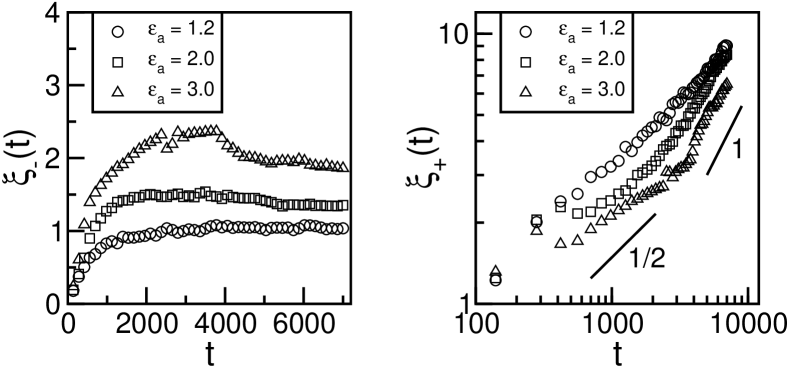
Figure 4: Time-dependence of the fit parameters $\xi_{-}$ (left panel) and $\xi_{+}$ (right panel) of SE profiles. The surface field values are indicated in the legends. The length scale $\xi_{-}(t)$ rapidly saturates to its equilibrium value, whereas $\xi_{+}(t)$ shows a crossover from the diffusive regime ($\xi_{+}\sim t^{1/2}$) to the hydrodynamic regime ($\xi_{+}\sim t$) for higher surface field strengths ($\epsilon_{a}=2.0,3.0$). The lines of slope $1/2$ and $1$ are provided as a guide to the eye.

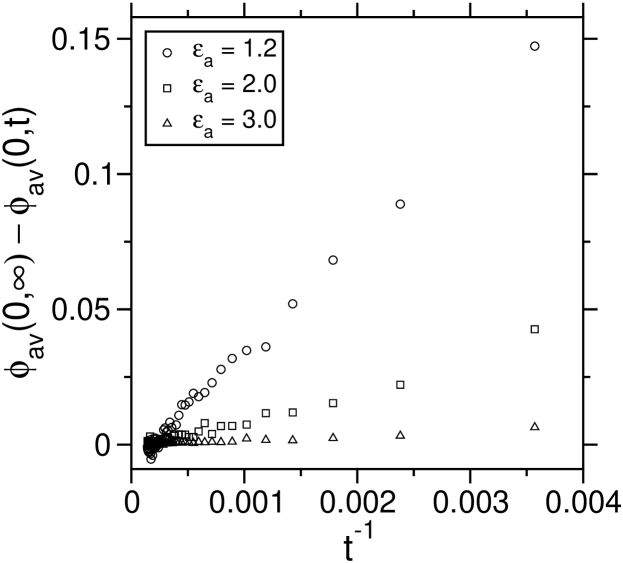
Figure 5: Time-dependence of the surface value of the order parameter for the SE profiles. We plot $\phi_{\textrm{av}}(0,\infty)-\phi_{\textrm{av}}(0,t)$ vs. $t^{-1}$ for $\epsilon_{a}=1.2,2.0,3.0$.

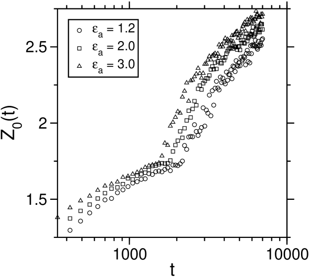
Figure 6: Time-dependence of the first zero crossing of the SE profiles. We plot $Z_{0}(t)$ vs. $t$ (note the logarithmic scale of time) for $\epsilon_{a}=1.2,2.0,3.0$. This plot confirms the crossover in the growth exponent from the diffusive regime to the hydrodynamic regime.

References

- [1] J. W. Cahn, J. Chem. Phys. 66, 3667 (1977).
- [2] M. E. Fisher, J. Stat. Phys. 34, 667 (1984).
- [3] M. E. Fisher, J. Chem. Soc. Faraday Trans. 282, 1569 (1986).
- [4] P. G. de Gennes, Rev. Mod. Phys. 57, 827 (1985).
- [5] S. Dietrich, in Phase Transitions and Critical Phenomena, edited by C. Domb and J. L. Lebowitz (Academic Press, London, 1988), Vol. 12, p. 1.
- [6] T. Young, Philos. Trans. R. Soc. Lond., Ser. A 95, 69 (1805).
- [7] A. J. Bray, Adv. Phys. 43, 357 (1994).
- [8] Kinetics of Phase Transitions, edited by S. Puri and V.K. Wadhawan (CRC Press, Boca Raton, Florida, 2009).
- [9] R. A. L. Jones, L. J. Norton, E. J. Kramer, F. S. Bates, and P. Wiltzius, Phys. Rev. Lett. 66, 1326 (1991).
- [10] G. Krausch, C.-A. Dai, E. J. Kramer, and F. S. Bates, Phys. Rev. Lett. 71, 3669 (1993).
- [11] G. Krausch, Mater. Sci. Eng. Rep. R14, 1 (1995).
- [12] M. Geoghegan and G. Krausch, Prog. Polym. Sci. 28, 261 (2003).
- [13] S. Puri and H. L. Frisch, J. Phys.: Condens. Matter 9, 2109 (1997).
- [14] S. Puri, J. Phys.: Condens. Matter 17, R101 (2005).
- [15] K. Binder, S. Puri, S. K. Das, and J. Horbach, J. Stat. Phys. 138, 51 (2010).
- [16] S. Puri and K. Binder, Phys. Rev. Lett. 86, 1797 (2001); Phys. Rev. E 66, 061602 (2002).
- [17] Y. S. Lipatov, in Encyclopedia of Surface and Colloid Science, edited by P. Somasundaran and A. T. Hubbard (Taylor and Francis, New York, 2006).
- [18] R. A. L. Jones, E. J. Kramer, M. H. Rafailovich, J. Sokolov, and S. A. Schwarz, Phys. Rev. Lett. 62, 280 (1989).
- [19] R. A. L. Jones and E. J. Kramer, Philos. Mag. B 62, 129 (1990).
- [20] M. Geoghegan, T. Nicolai, J. Penfold, and R. A. L. Jones, Macromolecules 30, 4220 (1997).
- [21] J. Genzer and R. J. Composto, Europhys. Lett. 38, 171 (1997).
- [22] H. Wang, J. F. Douglas, S. K. Satija, R. J. Composto, and C. C. Han, Phys. Rev. E 67, 061801 (2003).
- [23] O. G. Mouritsen (private communication).
- [24] J. M. Blakely, in Chemistry and Physics of Solid Surfaces, edited by R. Vanselow (Chemical Rubber, Boca Raton, 1979), Vol. 2.
- [25] P. Lejcek, J. Kovac, J. Vanickova, J. Ded, Z. S. Zija, and A. Zalar, Surface and Interface Analysis 42, (2010).
- [26] P. Guenoun, D. Beysens, and M. Robert, Phys. Rev. Lett. 65, 2406 (1990); Physica A 172, 137 (1991).
- [27] V. M. Kendon, M. E. Cates, I. Pagonabarraga, J.-C. Desplat, and P. Bladon, J. Fluid Mech. 440, 147 (2001).
- [28] A. J. Wagner and M. E. Cates, Europhys. Lett. 56, 556 (2001).
- [29] S. Ahmad, S. K. Das, and S. Puri, arXiv:1005.5096 (2010).
- [30] H. Tanaka, J. Phys.: Condens. Matter 13, 4637 (2001).
- [31] S. Bastea, S. Puri, and J. L. Lebowitz, Phys. Rev. E 63, 041513 (2001).
- [32] P. K. Jaiswal, S. Puri, and S. K. Das, in preparation.
- [33] S. K. Das, S. Puri, J. Horbach, and K. Binder, Phys. Rev. Lett. 96, 016107 (2006); Phys. Rev. E 73, 031604 (2006).
- [34] S. K. Das, J. Horbach, and K. Binder, J. Chem. Phys. 119, 1547 (2003).
- [35] S. K. Das, J. Horbach, K. Binder, M. E. Fisher, and J. V. Sengers, J. Chem. Phys. 125, 024506 (2006).
- [36] S. K. Das, M. E. Fisher, J. V. Sengers, J. Horbach, and K. Binder, Phys. Rev. Lett. 97, 025702 (2006).
- [37] M. P. Allen and D. J. Tildesley, Computer Simulation of Liquids (Clarendon Press, Oxford, 1987).
- [38] Monte Carlo and Molecular Dynamics of Condensed Matter Systems, edited by K. Binder and G. Ciccotti (Italian Physical Society, Bologna, 1996).
- [39] Z. Jiang and C. Ebner, Phys. Rev. B 39, 2501 (1989).
- [40] R. Toral and A. Chakrabarti, Phys. Rev. B 43, 3438 (1991).
- [41] K. Binder and H. L. Frisch, Z. Phys. B 84, 403 (1991).
- [42] S. Puri and H. L. Frisch, J. Chem. Phys. 79, 5560 (1993).
- [43] H. L. Frisch, S. Puri, and P. Nielaba, J. Chem. Phys. 110, 10514 (1999).
- [44] S. Puri and K. Binder, Phys. Rev. A 46, R4487 (1992); Phys. Rev. E 49, 5359 (1994); J. Stat. Phys. 77, 145 (1994); S. Puri, K. Binder, and H. L. Frisch, Phys. Rev. E 56, 6991 (1997).
- [45] P. C. Hohenberg and B. I. Halperin, Rev. Mod. Phys. 49, 435 (1977).