Continual Reassessment and Related Dose-Finding Designs

Abstract

During the last twenty years there have been considerable methodological developments in the design and analysis of Phase 1, Phase 2 and Phase 1/2 dose-finding studies. Many of these developments are related to the continual reassessment method (CRM), first introduced by O’Quigley, Pepe and Fisher (1990). CRM models have proven themselves to be of practical use and, in this discussion, we investigate the basic approach, some connections to other methods, some generalizations, as well as further applications of the model. We obtain some new results which can provide guidance in practice.

and

1 Introduction

The continual reassessment method (CRM) was introduced by O’Quigley, Pepe and Fisher (1990) as a design with which to carry out and analyze dose-finding studies in oncology. The purpose of these studies, usually referred to as Phase 1 trials of a new therapeutic agent, is to estimate the maximum tolerated dose (MTD) to be used in Phase 2 and Phase 3 trials. O’Quigley, Pepe and Fisher (1990) pointed out that standard methods in use then, and still in use now, fail to address the basic ethical requirements of experimentation with human subjects. Given the unknown or poorly understood relationship between dose and the probability of undesirable side effects (toxicity), it is inevitable, during experimentation, that some patients will be treated at too toxic doses and some patients will be treated at doses too low to have any real chance of procuring benefit. Aside from being inefficient, the case against the standard designs is that more patients than necessary are treated in this way, either at too toxic a dose or, more usually, at too low a dose to provide therapeutic benefit.

The rationale of the CRM is to concentrate as many patients as we can on doses at, or close to, the MTD. Doing so can provide an efficient estimate of the MTD while maximizing the number of patients in the study treated at doses with potential therapeutic benefit but without undue risk of toxicity. A drawback of concentrating patients to a small number of dose levels, at and around the MTD, is that the overall dose-toxicity curve itself may be difficult to estimate. In practice, this tends not to be a serious drawback, since estimation of the entire dose-toxicity curve is rarely the goal of a dose-finding clinical trial.

Phase 1 trials evaluating the toxicity of single agents are becoming less common, giving way to more complex studies involving multiple agents at various doses, heterogeneous groups of patients, and evaluations of both toxicity and efficacy. The standard methods are ill-equipped to handle these more complex situations, and here, we will discuss developments of the CRM and related methods for tackling various problems which arise in the context of dose finding. Whereas the standard method, even for the simplest situation fails to perform adequately, model based designs, while offering greatly improved performance for the simplest case, allow us to take on board those more involved situations that arise in practice (Braun, 2002; Faries, 2004; Goodman, Zahurak and Piantadosi, 1995; Legedeza and Ibrahim, 2002; Mahmood, 2001; O’Quigley, 2002a; O’Quigley and Paoletti, 2003; O’Quigley and Reiner, 1998;O’Quigley, Shen and Gamst, 1999; Piantadosi and Liu, 1996).

We begin with the definitions and notation used in Phase 1 trials and an overview of the CRM as originally proposed by O’Quigley, Pepe and Fisher (1990). The next two sections outline Bayesian and likelihood-based inference for the CRM, providing results for the small-sample and large-sample properties of the method. Section 5 gives extensions of the method and discusses modifications of the basic design. Section 6 presents related designs, again for the case of a single outcome whereas Section 7 considers two outcomes, one positive and one negative and describes the goal of locating the most successful dose (MSD). The article concludes with a discussion of future directions in the study of model-based methods for dose-finding studies.

1.1 Doses, DLT, MTD and the MSD

Traditional thinking in the area of cytotoxic anti-cancer treatments is to give as strong a treatment as we can without incurring too much toxicity. For the great majority of new cancer treatments—recent advances in immunotherapy being possible exceptions—we consider that increases in dose correspond to increases in both the number of patients who will experience toxic side effects as well as the numbers who may benefit from treatment. If we observe a complete absence of toxic side effects, then we would not anticipate observing any therapeutic effect, either for those patients in the study or for future patients. The Phase I trial then has for its goal the determination of some dose having an “acceptable” rate of toxicity. While it is true that the essential goal of the study is to improve treatment for future patients, ethical concerns dictate that we give the best possible treatment to the patients participating in the Phase I study itself. The highest dose level at which patients can be treated and where the rate of toxicity is deemed to be still acceptable is known as the MTD (maximal tolerated dose).

On an individual level we can imagine being able to increase the dose without encountering the toxic effect of interest. At some threshold the individual will suffer a toxicity. An assumed model is the following: at this threshold the individual suffers a toxicity and, for all higher doses, the individual would also have encountered a toxicity. Such a model is reasonable for most situations and widely assumed. It remains nonetheless a model and might be brought under scrutiny in particular cases. The model stipulates that for all levels below the threshold, the individual would not suffer any toxicity and we call the threshold itself the individual’s own maximum tolerated dose (MTD). A dose-limiting toxicity (DLT) curve for the individual would be a $(0,1)$ step function, the value 0 indicating no toxicity and the value 1 a toxicity. Thus, in the case of an individual, the $(0,1)$ step function for the DLT coincides with that for the MTD.

Any population of interest can be viewed as being composed of individuals each having their own particular MTD. Corresponding to each individual MTD we have a $(0,1)$ step function for the individual’s DLT. Over some set or population of individuals, the sum of the DLT curves at any dose equates to the probability of toxicity at that same dose. For a population we fix some percentile so that, $100\times\theta\%$ say, have their own threshold at or below this level. The term MTD is often used somewhat loosely, and not always well defined. The more precise definition given in terms of a percentile involves $\theta.$ Different values of $\theta$ would correspond to different definitions of the MTD. The values 0.2, 0.25 and 0.33 are quite common in practice.

When information on efficacy, possibly through surrogate measures or otherwise through some measure of response, is available in a timely way, then it makes sense to make use of such information. In the HIV setting, there have been attempts to simultaneously address the problems of both toxicity and efficacy. The goal then becomes not one of finding the maximum tolerated dose but, rather, one of finding the MSD (most successful dose), that is, that dose where the probability of treatment failure, be it due to excessive toxicity or to insufficient evidence of treatment efficacy, is a minimum. The CRM can be readily adapted to address these kinds of questions (O’Quigley, Hughes and Fenton, 2001; Zohar and O’Quigley, 2006a).

1.2 Notation

We assume that we have available $k$ doses; $d_{1},\ldots,\break d_{k}$, possibly multidimensional and ordered in terms of the probabilities, $R(d_{i})$, for toxicity at each of the levels, that is, $R(d_{i})<R(d_{j})$ whenever $i<j$. The MTD is denoted $d_{0}$ and is taken to be one of the values in the set $\{d_{1},\ldots,d_{k}\}.$ It is the dose that has an associated probability of toxicity, $R(d_{0})$, as close as we can get to some target “acceptable” toxicity rate $\theta$. Specifically we define $d_{0}\in\{d_{1},\ldots,d_{k}\}$ such that

$$|R(d_{0})-\theta|$$

(1)

$$\quad<|R(d_{\ell})-\theta|,\quad\ell=1,\ldots,k;d_{\ell}\neq d_{0}.$$

The binary indicator $Y_{j}$ takes the value $1$ in the case of a toxic response for the $j$th entered subject ($j=1,\ldots,n$) and 0 otherwise. The dose for the $j$th entered subject, $X_{j}$, is viewed as random taking values $x_{j}\in\{d_{1},\ldots,d_{k}\};j=1,\ldots,n.$ Thus we can write

$$\Pr(Y_{j}=1|X_{j}=x_{j})=R(x_{j}).$$

Little is known about $R(\cdot)$ and, given the $n$ observations, the main goal is to identify $d_{0}$. Estimation of all or part of $R(d_{\ell}),$ $\ell=1,\ldots,k,$ is only of indirect interest in as much as it may help provide information on $d_{0}.$

There is an extensive literature on problems similar to that just described. The solutions to these problems, however, are mostly inapplicable in view of ethical constraints involved in treating human subjects. The patients included in the Phase I design must, themselves, be treated “optimally,” the notion optimal now implying for these patients a requirement to treat at the best dose level, taken to be the one as close as we can get to $d_{0}$. We then have two statistical goals: (1) estimate $d_{0}$ consistently and efficiently and, (2) during the course of the study, concentrate as many experiments as possible around $d_{0}$. Specifically, we aim to treat the $j$th included patient at the same level we would have estimated as being $d_{0}$ had the study ended after the inclusion of $j-1$ patients.

2 Continual Reassessment Method

The continual reassessment method (CRM), proposed as a statistical design to meet the requirements of the type of studies described above, was introduced by O’Quigley, Pepe and Fisher (1990). Many developments and innovations have followed, the basic method and variants having found a number of other potential applications. Here, we reconsider the original problem, expressed in statistical terms, since it is this problem that forged the method. In this article we consider the main theoretical ideas and do not dwell on precise applications apart from for illustrative purposes.

The method begins with a parameterized working model for $R(x_{j})$, denoted by $\psi(x_{j},a)$, for some one-parameter model $\psi(x_{j},a)$ and $a$ defined on the set $\mathcal{A}$. For every $a$, $\psi(x,a)$ should be monotone increasing in $x$ and, for any $x$, $\psi(x,a)$ should be monotone in $a$. For every $d_{i}$ there exists some $a_{i}\in{\mathcal{A}}$ such that $R(d_{i})=\psi(d_{i},a_{i})$, that is, the one-parameter model is rich enough, at each dose, to exactly reproduce the true probability of toxicity at that dose. There are many choices for $\psi(x,a)$, including the simple Lehmann type shift model:

$$\log\{-\log\psi(d_{i},a)\}$$

(2)

$$\quad=\log\{-\log\alpha_{i}\}+a,\quad i=1,\ldots,k,$$

where $0<\alpha_{1}<\cdots<\alpha_{k}<1$ and $-\infty<a<\infty$, having shown itself to work well in practice. This parameterization allows for the support of the parameter $a$ to be on the whole real line and priors such as the normal or the logistic, having heavier tails, have been used here. The simple power model of O’Quigley, Pepe and Fisher (1990) required that support for the parameter $a$ be restricted to the positive real line.

O’Quigley, Pepe and Fisher (1990) suggested that the ${\alpha_{i}},i=1,\ldots,k$, be chosen to reflect a priori assumptions about the toxicity probabilities associated with each dose. Lee and Cheung (2009) provided a systematic approach to choosing the initial values for the ${\alpha_{i}},i=1,\ldots,k$. Yin and Yuan (2009) used Bayesian model averaging to combine estimates from different sets of initial guesses at the ${\alpha_{i}},i=1,\ldots,k$. It should again be noted that the working model is not anticipated to represent the entire dose-toxicity curve. It suffices that the parameterized working model be flexible enough to allow for estimation of the dose-toxicity relationship at and close to the MTD. This point will be developed more fully in Section 4, which summarizes the small- and large-sample properties of the CRM. Cheung and Chappell (2002) investigated the operational sensitivity to different model choices.

Once a model has been chosen and we have data in the form of the set $\Omega_{j}=\{y_{1},x_{1},\ldots,y_{j},x_{j}\}$, the outcomes of the first $j$ experiments, we obtain estimates ${\hat{R}}(d_{i})$ $(i=1,\ldots,k)$ of the true unknown probabilities $R(d_{i})$ $(i=1,\ldots,k)$ at the $k$ dose levels (see below). The target dose level is that level having associated with it a probability of toxicity as close as we can get to $\theta$. The dose or dose level $x_{j}$ assigned to the $j$th included patient is such that

$$|{\hat{R}}(x_{j})-\theta|$$

(3)

$$\quad<|{\hat{R}}(d_{\ell})-\theta|,\quad\ell=1,\ldots,k;d_{\ell}\neq x_{j}.$$

This equation should be compared to (1.2). It translates the idea that the overall goal of the study is also the goal for each included patient. The CRM is then an iterative sequential design, the level chosen for the $(n+1)$th patient, who is hypothetical, being also our estimate of $d_{0}.$ After having included $j$ subjects, we can calculate a posterior distribution for $a$ which we denote by $f(a,\Omega_{j}).$ We then induce a posterior distribution for ${\psi}(d_{i},a)$, $i=1,\ldots,k,$ from which we can obtain summary estimates of the toxicity probabilities at each level so that

$${\hat{R}}(d_{i})$$

(4)

$$\quad=\int_{a\in\mathcal{A}}\psi(d_{i},a)f(a,\Omega_{j})\,da,\quad i=1,\ldots,k.$$

Using (2) we can now decide which dose level to allocate to the $(j+1)$th patient.

In the original version of the CRM, O’Quigley, Pepe and Fisher (1990) used an alternative estimate ${\tilde{R}}(d_{i})=\psi(d_{i},\mu)$, $i=1,\ldots,k,$ where $\mu=\break\int_{a\in\mathcal{A}}af(a,\Omega_{j})\,da.$ This was done primarily to reduce the amount of calculation required, a consideration of less importance today. O’Quigley, Pepe and Fisher (1990) completed the specification of the dose allocation algorithm by specifying a starting dose based on a prior specification of the dose level with probability closest to the target.

3 Bayesian and Likelihood Inference

In order to base inference only on the likelihood it is necessary to have the likelihood nonmonotone so that the estimates are not on the boundary of the parameter space. This is accomplished by having some initial escalation scheme until the data achieve at least one toxicity and one nontoxicity. We can regard the data obtained via this initial escalation scheme as, in some sense, empirical and use them as a data-based prior to the second part of the study. Thus, both Bayesian and likelihood alone, can all be put under a Bayesian heading. We use this in the following to study different Bayesian approaches to inference.

3.1 Likelihood-Based Dose Allocations

After the inclusion of the first $j$ patients, the logarithm of the likelihood can be written as

$${\mathcal{L}}_{j}(a) = \sum_{\ell=1}^{j}y_{\ell}\log\psi(x_{\ell},a)$$

$${}+\sum_{\ell=1}^{j}(1-y_{\ell})\log\bigl{(}1-\psi(x_{\ell},a)\bigr{)},$$

where any terms not involving the parameter $a$ have been equated to zero. We suppose that ${\mathcal{L}}_{j}(a)$ is maximized at $a=\hat{a}_{j}$. Once we have calculated $\hat{a}_{j}$ we can next obtain an estimate of the probability of toxicity at each dose level $d_{i}$ via ${\hat{R}}(d_{i})=\psi(d_{i},\hat{a}_{j})$ $(i=1,\ldots,k).$ On the basis of this formula the dose to be given to the $(j+1)$th patient, $x_{j+1}$, is determined. Once we have estimated $a$ we can also calculate an approximate 100$(1-\alpha)\%$ confidence interval for $\psi(x_{j+1},{\hat{a}}_{j})$ as $(\psi_{j}^{-},\psi_{j}^{+})$ where

$$\psi_{j}^{-} = \psi\bigl{\{}x_{j+1},\bigl{(}{\hat{a}}_{j}+z_{1-\alpha/2}v({\hat{a}}_{j})^{1/2}\bigr{)}\bigr{\}},$$

$$\psi_{j}^{+} = \psi\bigl{\{}x_{j+1},\bigl{(}{\hat{a}}_{j}-z_{1-\alpha/2}v({\hat{a}}_{j})^{1/2}\bigr{)}\bigr{\}},$$

where $z_{\alpha}$ is the $\alpha$th percentile of a standard normal distribution and $v({\hat{a}}_{j})$ is an estimate of the variance of ${\hat{a}}_{j}$. For the model of (2) this turns out to be particularly simple and we can write

$$v^{-1}({\hat{a}}_{j}) = \sum_{\ell\leq j,y_{\ell}=0}\psi(x_{\ell},{\hat{a}}_{j})(\log\alpha_{\ell})^{2}$$

$$\hphantom{\sum_{\ell\leq j,y_{\ell}=0}}{}/\bigl{(}1-\psi(x_{\ell},{\hat{a}}_{j})\bigr{)}^{2}.$$

Although based on a misspecified model these intervals turn out to be quite accurate, even for sample sizes as small as 16, and thus helpful in practice (O’Quigley, 1992).

3.2 Prior Information on the Parameter $a$

There are three distinct approaches which can be used in order to establish the prior information. These are: (1) postulate some numerically tractable and sufficiently flexible density $g(a)$, (2) introduce apseudo-data prior which indirectly will specify $g(a)$, and (3) use some initial escalation scheme in a two-stage design until the first toxicity is observed. Let us consider these three approaches more closely.

A gamma prior for $g(a)$

For the Lehmann shift model, on a logarithmic scale, given that ${\mathcal{A}}=(0,\infty),$ O’Quigley, Pepe and Fisher (1990) suggested, as a natural candidate,

$$g(a)=\lambda^{c}a^{c-1}\exp\{-(\lambda a)\}/\Gamma(c),$$

$$\eqntext{\displaystyle\Gamma(c)=\int_{0}^{\infty}\exp(-u)u^{c-1}\,du}$$ (6)

the gamma density with scale parameter $\lambda$ and shape parameter $c$. The necessary steps in fitting a gamma prior on the basis of the upper and lower points of our prior confidence region have been described by Martz and Waller (1982). For a relatively simple set-up involving no more than six doses and using a coding for dose (not the actual dose itself), O’Quigley, Pepe and Fisher (1990) suggested that the simple exponential prior for $a$—a special case of the gamma prior with $c$ and $\lambda$ both equal to 1—would be satisfactory. Some authors have appealed to this simple exponential prior in different contexts, or more involved set-ups, and the resulting behavior of the method can be alarming (Moller, 1995).

Pseudo-data prior

In the place of a prior expressed as a specific parametric density function, pseudo-data priors create observations that are weighted in accordance with our degree of belief in their plausibility. Using pseudo-data ${y^{*}_{\ell}},\ell=1,\ldots,K$, the prior $g(a)$ is defined from

$$\qquad g(a) \cong \exp\Biggl{[}\sum_{\ell=1}^{j}y^{*}_{\ell}\log\psi(x_{\ell},a)$$

$$\hphantom{\exp\Biggl{[}}{}+\sum_{\ell=1}^{j}(1-y^{*}_{\ell})\log\bigl{(}1-\psi(x_{\ell},a)\bigr{)}\Biggr{]}.$$

The prior “data” can be combined with the observed data. In consequence standard and widely available programs such as SAS or SPSS may be used directly to calculate the posterior mode without the need for numerical integration. The pseudo-data prior can be used to establish our best prior guesses which will be mirrored by the estimates of $a$ obtained from fitting the pseudo-data alone. The imprecision which we wish to associate with this can be governed by a weighting coefficient $w_{j}$ where $0<w_{j}<1.$ This coefficient can be independent of $j$ and we would usually require that $w_{j}\leq w_{j-1}.$ The posterior density is then

$$f(a,\Omega_{j}) = A^{-1}_{j}\exp\{w_{j}\log g(a)$$

$$\hphantom{A^{-1}_{j}\exp\{}{}+(1-w_{j}){\mathcal{L}}_{j}(a)\},$$

where $A_{j}=\!\int_{-\infty}^{\infty}\exp\{w_{j}\!\log g(a)+(1-w_{j}){\mathcal{L}}_{j}(a)\}\,da.$ The added generality of allowing the dependence of the weights on $j$ would rarely be needed and, in most practical situations, it suffices to take $w$ as a constant small enough so that the prior has no more impact than deemed necessary.

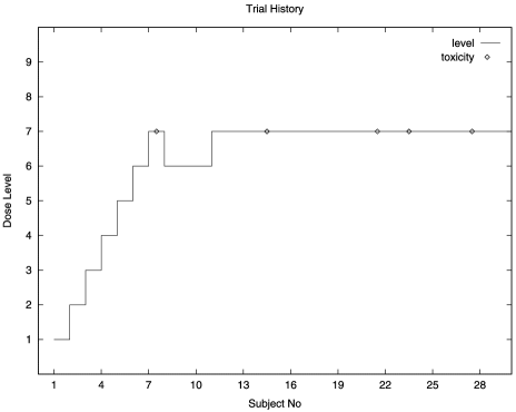
Figure 1: A typical trial history using rapid early escalation; target is level 7.

Uninformative priors

For the model (2), O’Quigley (1992) suggested a normal prior having mean zero and variance $\sigma^{2}$, large enough to be considered noninformative. Such a concept can be made more precise in the following way, at least for fixed sample designs. The mean and mode of the prior are at zero so that, should the true probabilities of toxicity exactly coincide with the $\alpha_{i}$ then, the more informative the prior the better we do, ultimately as the prior tends to being degenerate, that is, $\sigma^{2}\to 0$, we obtain the correct level always. Taking some distance measure between the distribution of our final recommendation and the degenerate distribution putting all mass on the correct level, this distance will increase as our uncertainty, as measured by $\sigma^{2}$, increases. The curve of this distance, as a function of $\sigma^{2}$, will reach an asymptotic limit, further increases in $\sigma^{2}$ having a vanishing influence on the error distribution of final recommendation. The smallest finite value of $\sigma^{2}$, such that the operating characteristics are sufficiently close to those obtained when $\sigma^{2}$ is infinite (in practice very large), corresponding to a diffuse and even improper prior, will provide the prior with the required behavior.

An uninformative prior, in the sense that it does not favor any particular level, can be constructed readily in the light of the results of O’Quigley (2006) which partition the interval $[A,B]$ for the parameter $a$ into $k$ subintervals $S_{i}$ $(i=1,\ldots,k).$ If $a\in S_{i},$ then dose level $d_{i}$ corresponds to the MTD. For $k$ dose levels we simply associate the probability mass $1/k$ to each of the $k$ subsets $S_{i}.$ Clearly this approach is readily extended to the informative case by putting priors favoring some levels more than others, either on the basis of clinical information or simply out of a desire to influence the operating characteristics in some particular way. An example for the frequent case $k=6$ would be to associate the prior 0.05 with level 1, and the values 0.19 with the other five levels. This would result in steering us away from level 1 in favor of the other levels, unless the accumulating data begin to weigh against our conjecture that level 1 is unlikely to be the right level.

Data-based prior in two-stage designs

In order to be able to maximize the log-likelihood on the interior of the parameter space we require heterogeneity among the responses, that is, at least one toxic and one nontoxic response (Silvapulle, 1981). Otherwise the likelihood is maximized on the boundary of the parameter space and our estimates of $R(d_{i})$ $(i=1,\ldots,k)$ are trivially either zero, 1, or, depending on the model we are working with, may not even be defined. In the context of “pure likelihood”-based designs O’Quigley and Shen (1996) argued for two-stage designs whereby an initial escalation scheme provided the required heterogeneity. The experiment can be viewed as not being fully underway until we have some heterogeneity in the responses. These could arise in a variety of different ways: use of a standard Up and Down approach, use of an initial Bayesian CRM as outlined below, or use of a design believed to be more appropriate by the investigator. Once we have achieved heterogeneity, the model kicks in and we continue as prescribed above (estimation–allocation). We can also consider this initial escalation as providing empirical data. Conditional upon these data we then proceed to the second stage. The data obtained at the end of the first stage can be viewed as providing an empirical prior. In this way, all the approaches can be grouped under a Bayesian umbrella. The essential differences arise through the different ways of specifying the prior.

Using empirical data to construct a prior as the first stage of a two-stage design can afford us a great deal of flexibility. The initial exploratory escalation stage is followed by a more refined homing in on the target. Such an idea was first proposed by Storer (1989) in the context of the more classical Up and Down schemes. His idea was to enable more rapid escalation in the early part of the trial where we may be quite far from a level at which treatment activity could be anticipated. Moller (1995) was the first to use this idea in the context of CRM designs. Her idea was to allow the first stage to be based on some variant of the usual Up and Down procedures. In the context of sequential likelihood estimation, the necessity of an initial stage was pointed out by O’Quigley and Shen (1996) since the likelihood equation fails to have a solution on the interior of the parameter space unless some heterogeneity in the responses has been observed. Their suggestion was to work with any initial scheme, Bayesian CRM or Up and Down, and, for any reasonable scheme, the operating characteristics appear relatively insensitive to this choice.

Table 1: Toxicity “grades” (severities) for trial

Severity	Degree of toxicity
0	No toxicity
1	Mild toxicity (non-dose-limiting)
2	Nonmild toxicity (non-dose-limiting)
3	Severe toxicity (non-dose-limiting)
4	Dose-limiting toxicity

Here we describe an example of a two-stage design that has been used in practice (see Figure 1). There were many dose levels and the first included patient was treated at a low level. As long as we observe very low-grade toxicities then we escalate quickly, including only a single patient at each level. As soon as we encounter more serious toxicities then escalation is slowed down. Ultimately we encounter dose-limiting toxicities at which time the second stage, based on fitting a CRM model, comes fully into play. This is done by integrating this information and that obtained on all the earlier non-dose-limiting toxicities to estimate the most appropriate dose level. Consider the following example which uses information on low-grade toxicities in the first stage in order to allow rapid initial escalation (see Table 1). Specifically we define a grade severity variable $S(i)$ to be the average toxicity severity observed at dose level $i$, that is, the sum of the severities at that level divided by the number of patients treated at that level. The rule is to escalate providing $S(i)$ is less than 2. Furthermore, once we have included three patients at some level, then escalation to higher levels only occurs if each cohort of three patients does not experience dose-limiting toxicity. This scheme means that, in practice, as long as we see only toxicities of severities coded 0 or 1, then we escalate. The first severity coded 2 necessitates a further inclusion at this same level and, anything other than a 0 severity for this inclusion, would require yet a further inclusion and a non-dose-limiting toxicity before being able to escalate. This design also has the advantage that, should we be slowed down by a severe (severity 3), albeit non-dose-limiting toxicity, we retain the capability of picking up speed (in escalation) should subsequent toxicities be of low degree (0 or 1). This can be helpful in avoiding being handicapped by an outlier or an unanticipated and possibly not drug-related toxicity arising early in the study. Once a dose-limiting toxicity is encountered the initial escalation stage is brought to a halt and the accumulated data taken as our empirical prior.

3.3 An Illustration

An example of a two-stage design involving 16 patients was given by O’Quigley and Shen (1996). There were six levels in the study, maximum likelihood was used, and the first entered patients were treated at the lowest level. The design was two-stage. The true toxic probabilities were $R(d_{1})=0.03$, $R(d_{2})=0.22$, $R(d_{3})=0.45$, $R(d_{4})=0.6$, $R(d_{5})=0.8$ and $R(d_{6})=0.95$. The working model was that given by (2) where $\alpha_{1}=0.04$, $\alpha_{2}=0.07$, $\alpha_{3}=0.20$, $\alpha_{4}=0.35$, $\alpha_{5}=0.55$ and $\alpha_{6}=0.70$. The targeted toxicity was given by $\theta=0.2$ indicating that the best level for the MTD is given by level 2 where the true probability of toxicity is 0.22. A grouped design was used until heterogeneity in toxic responses was observed, patients being included, as for the classical schemes, in groups of three. The first three patients experienced no toxicity at level 1. Escalation then took place to level 2 and the next three patients treated at this level did not experience any toxicity either. Subsequently two out of the three patients treated at level 3 experienced toxicity. Given this heterogeneity in the responses the maximum likelihood estimator for $a$ now exists and, following a few iterations, could be seen to be equal to 0.715. We then have that $\hat{R}(d_{1})=0.101$, $\hat{R}(d_{2})=0.149$, $\hat{R}(d_{3})=0.316$, $\hat{R}(d_{4})=0.472$, $\hat{R}(d_{5})=0.652$ and $\hat{R}(d_{6})=0.775$. The 10th entered patient is then treated at level 2 for which $\hat{R}(d_{2})=0.149$ since, from the available estimates, this is the closest to the target $\theta=0.2$. The 10th included patient does not suffer toxic effects and the new maximum likelihood estimator becomes 0.759. Level 2 remains the level with an estimated probability of toxicity closest to the target. This same level is in fact recommended to the remaining patients so that after 16 inclusions the recommended MTD is level 2. The estimated probability of toxicity at this level is 0.212 and a 90% confidence interval for this probability is estimated as (0.07, 0.39).

4 Large-Sample and Small-Sample Properties

Extensive simulations (O’Quigley, Pepe and Fisher, 1990; O’Quigley and Shen, 1996; O’Quigley, 1999; Iasonos et al., 2008), over wide choices of possible true unknown dose-toxicity situations, show the method to behave in a mostly satisfactory way, recommending the right level or close levels in a high percentage of situations and treating in the study itself a high percentage of included patients, again, at the right level or levels close by. Cheung (2005), O’Quigley (2006) and Lee and Cheung (2009) obtained theoretical results which not only provide some confidence in using the method but can also provide guidance in the choice and structure of working models. Even though models are misspecified, inference is still based on an estimating equation taken from the derivative of the log-likelihood. Thus, Shen and O’Quigley (1996) defined

$$I_{n}(a)=\frac{1}{n}\sum_{j=1}^{n}\biggl{[}y_{j}\frac{\psi^{\prime}}{\psi}\{x_{j},a\}+(1-y_{j})\frac{-\psi^{\prime}}{1-\psi}\{x_{j},a\}\biggr{]}.$$

Some restrictions on $\psi$ are needed (O’Quigley, 2006). In particular, there must exist constants $a_{1},\ldots,a_{k}$ $\in[A,B]$ such that $\psi(d_{i},a_{i})=R_{i}$, the function $\psi$ satisfies $\psi(d_{i},B)<\theta<\psi(d_{i},A)$, and there is a unique $a_{0}\in(a_{1},\ldots,a_{k})$, $\psi(d_{0},a_{0})=R(d_{0})=\theta_{0}.$ In general, $\theta_{0}$ will not be equal to $\theta$ but will be as close as we can get given the available doses. We require the estimating function to respect a standard condition of estimating functions which is that

$$s(t,x,a)=t\frac{\psi^{\prime}}{\psi}\{x,a\}+(1-t)\frac{-\psi^{\prime}}{1-\psi}\{x,a\}$$

is continuous and strictly monotone in $a$. We define $\tilde{I}_{n}(a)=n^{-1}\sum_{j=1}^{n}s\{R(x_{j}),x_{j},a\}$.

It is not typically the case that $\psi(d_{i},a_{0})=R(d_{i})$ for $i=1,\ldots,k$. However, at least in the vicinity of the MTD, this will be approximately true, an idea that can be formalized (Shen and O’Quigley, 1996) via the definition of the set

$$\qquad S(a_{0}) = \{a\dvtx|\psi(d_{0},a)-\theta|<|\psi(d_{i},a)-\theta|$$

$$\hskip 92.0pt\mbox{for all }d_{i}\not=d_{0}\}.$$

Shen and O’Quigley (1996) showed that convergence follows if, for $i=1,\ldots,k$, $a_{i}\in S(a_{0})$. O’Quigley(2006) showed that, for each $1\leq i\leq k-1$, there exists a unique constant $\kappa_{i}$ such that $\theta-\psi(x_{i},\kappa_{i})=\psi(x_{i+1},\kappa_{i})-\theta>0.$ The constants $\kappa_{i}$ naturally give rise to a partitioning of the parameter space $[A,B].$ Letting $\kappa_{0}=A$ and $\kappa_{k}=B$, we can write the interval $[A,B]$ as a union of nonoverlapping intervals whereby $[A,B]=\bigcup_{i=1}^{k}[\kappa_{i-1},\kappa_{i}).$ This partition is of particular value in establishing prior distributions which can translate immediately into priors for the dose levels themselves. It is also of value in deriving results concerning the coherence, stability and convergence of the algorithm (Cheung and Chappell, 2002; O’Quigley, 2006).

Convergence to the MTD stems from the fact that $\sup_{a\in[A,B]}|I_{n}(a)-\tilde{I}_{n}(a)|$ converges almost surely to zero (Shen and O’Quigley, 1996) and that we can re-express $\tilde{I}_{n}(a)$ as a sum over the $k$ dose levels rather than a sum over the $n$ subjects; in particular we have that $\tilde{I}_{n}(a)=\sum_{i=1}^{k}\pi_{n}(d_{i})s\{R(d_{i}),d_{i},a\}.$ Supposing that the solution to the equation $\tilde{I}_{n}(a)=0$ is $\tilde{a}_{n}$ and that $a_{i}$ is the unique solution to the equation $s\{R(d_{i}),d_{i},a\}=0$, then $\tilde{a}_{n}$ will fall into the interval $S_{1}(a_{0})$. Since $\hat{a}_{n}$ solves $I_{n}(a)=0$, then, almost surely, $\hat{a}_{n}\in S(a_{0}),$ so that, for $n$ sufficiently large, $x_{n+1}\equiv d_{0}.$ Since there are only a finite number of dose levels, $x_{n}$ will ultimately settle at $d_{0}.$ Rather than appeal to the set $S(a_{0}),$ which quantifies the roughness of the working approximation to the true dose-toxicity function in the vicinity of the MTD, and which guarantees convergence to the MTD when all of the $a_{i}$ belong to this set, Cheung (2005) used a related approach which appeals to a more flexible—in many ways more realistic—definition of the MTD whereby probabilities of toxicity within some given range are all taken to be acceptable. Convergence can then be shown to obtain without such restrictive conditions as those described above.

4.1 Efficiency

O’Quigley (1992) proposed using $\hat{\theta}_{n}=\psi(x_{n+1},\hat{a}_{n})$ to estimate the probability of toxicity at the recommended level $x_{n+1}$, where $\hat{a}_{n}$ is the maximum likelihood estimate. An application of the $\delta$-method (Shen and O’Quigley, 1996) shows that the asymptotic distribution of $\sqrt{n}\{\hat{\theta}_{n}-R(d_{0})\}$ is $N\{0,\theta_{0}(1-\theta_{0})\}$. The estimate then provided by CRM is fully efficient for large samples. This is what our intuition would suggest given the convergence properties of CRM. What actually takes place in finite samples needs to be investigated on a case by case basis. The relatively broad range of cases studied by O’Quigley (1992) show a mean squared error for the estimated probability of toxicity at the recommended level under CRM to correspond well with the theoretical variance for samples of size $n$, were all subjects to be experimented at the correct level. Some of the cases studied showed evidence of super-efficiency, translating nonnegligible bias that happens to be in the right direction, while a few others indicated efficiency losses large enough to suggest the possibility of better performance.

A useful tool in studies of finite sample efficiency is the idea of an optimal design. We can derive a nonparametric optimal design (O’Quigley, Paoletti and Maccario, 2002) based upon no more than a monotonicity assumption. Such an optimal design is not generally available in practice but can serve as a gold standard in theoretical studies, playing a role similar to that of the Cramer–Rao bound. Comparisons between any suggested method and the optimal design enable us to quantify just how much room there is for potential improvement. Further evidence of the efficiency of the CRM was provided by the work of O’Quigley, Paoletti and Maccario (2002), where the CRM is compared to the nonparametric optimal design. In the cases studied in that article and in that of Paoletti, O’Quigley and Maccario (2004), potential for improvement is seen to be limited, with the identification of the MTD by the two-stage CRM design being only slightly inferior to that of the optimal design.

4.2 Nonidentifiability of Fully Parameterized Models

Under the conditions outlined above we will ultimately only include patients at dose level $d_{0}$. Under very much broader conditions (Shen and O’Quigley, 1996) we can guarantee convergence to some level, not necessarily $d_{0}$ but one where the probability of toxicity will not be far removed from that at $d_{0}$. The consequence of this is that, for the most common case of a single homogeneous group of patients, we are obliged to work with an underparameterized model, notably a one-parameter model in the case of a single group. Although a two-parameter model may appear more flexible, the convergence property of CRM means that ultimately we will not obtain information needed to fit two parameters. Having settled at dose level $d_{i}$, the only quantity we can estimate is $R(d_{i})$ which can be done consistently in light of the Glivenko–Cantelli lemma. Under our model conditions we have that $R(d_{i})=\psi(d_{i},a_{i})$ and that ${\hat{a}}_{j}$ will converge almost surely to $a_{i}$. Adding a second parameter can only overparameterize the situation and, for example, the commonly used logistic model has an infinite number of combinations of the two parameters which lead to the same value of $R(d_{i})$. A likelihood procedure can then be unstable and may even break down, whereas a two-parameter fully Bayesian approach (Gatsonis and Greenhouse, 1992; Whitehead and Williamson, 1998) may work initially, although somewhat artificially, but behave erratically as sample size increases and the structural rigidity provided by the prior gradually wanes. This is true even when starting out at a low or the lowest level, initially working with an Up and Down design for early escalation, before a CRM model is applied. Indeed, any design that ultimately concentrates all patients from a single group on some given level can fit no more than a single parameter without running into problems of identifiability.

5 Extended CRM Designs

The simple model of (2) can be extended to a class of models denoted by $\psi_{m}(x_{j},a)$ for $m=1,\ldots,M$ where there are $M$ members of the class. Take, for example,

$$\psi_{m}(d_{i},a)=\alpha_{mi}^{\exp(a)},$$

(10)

$$\eqntext{i=1,\ldots,k;m=1,\ldots,M,}$$ (11)

where $0<\alpha_{m1}<\cdots<\alpha_{mk}<1$ and $-\infty<a<\infty$, as an immediate generalization of (2). Prior information concerning the plausibility of each model is catered for by $\pi(m)$, $m=1,\ldots,M,$ where $\pi(m)\geq 0$ and where $\sum_{m}\pi(m)=1.$ When each model is given the same initial weighting, then we have that $\pi(m)=1/m.$ If the data are to be analyzed under model $m$, then, after the inclusion of $j$ patients, the logarithm of the likelihood can be written as

$${\mathcal{L}}_{mj}(a) = \sum_{\ell=1}^{j}y_{\ell}\log\psi_{m}(x_{\ell},a)$$

$${}+\sum_{\ell=1}^{j}(1-y_{\ell})\log\bigl{(}1-\psi_{m}(x_{\ell},a)\bigr{)},$$

where any terms not involving the parameter $a$ have been ignored. Under model $m$ we obtain a summary value of the parameter $a$, in particular the maximum of the posterior mode and we refer to this as ${\hat{a}}_{mj}$. Given the value of ${\hat{a}}_{mj}$ under model $m$, we have an estimate of the probability of toxicity at each dose level $d_{i}$ via ${\hat{R}}(d_{i})=\psi_{m}(d_{i},\hat{a}_{mj})$ $(i=1,\ldots,k).$ On the basis of this formula, and having taken some value for $m$, the dose to be given to the $(j+1)$th patient, $x_{j+1}$, is determined. Thus, we need some value for $m$ and we make use of the posterior probabilities of the models given the data $\Omega_{j}.$ Denoting these posterior probabilities by $\pi(m|\Omega_{j})$, then

$$\pi(m|\Omega_{j})$$

$$\quad=\frac{\pi(m)\int_{-\infty}^{\infty}\exp\{{\mathcal{L}}_{mj}(u)\}g(u)\,du}{\sum_{m=1}^{M}\pi(m)\int_{-\infty}^{\infty}\exp\{{\mathcal{L}}_{mj}(u)\}g(u)\,du}.$$

The estimated values of $\pi(m|\Omega_{j})$ can help us decide between models which have physical implications of interest to us. As an example suppose that there exists significant heterogeneity among the patients and this is simplified to the case of two groups.

5.1 A Simple Heterogeneity Model

As in other types of clinical trials we are essentially looking for an average effect. Patients naturally differ in the way they may react to a treatment and, although hampered by small samples, we may sometimes be in a position to specifically address the issue of patient heterogeneity. One example occurs in patients with acute leukemia where it has been observed that children will better tolerate more aggressive doses (standardized by their weight) than adults. Likewise, heavily pretreated patients are more likely to suffer from toxic side effects than lightly pretreated patients. In such situations we may wish to carry out separate trials for the different groups in order to identify the appropriate MTD for each group. Otherwise we run the risk of recommending an “average” compromise dose level, too toxic for a part of the population and suboptimal for the other. Usually, clinicians carry out two separate trials or split a trial into two arms after encountering the first DLTs when it is believed that there are two distinct prognostic groups. This has the disadvantage of failing to utilize information common to both groups. The most common situation is that of two samples where we aim to carry out a single trial keeping in mind potential differences between the two groups. A multisample CRM is a direct generalization although we must remain realistic in terms of what is achievable in the light of the available sample sizes.

Introduce a binary variable $Z$ taking the value 0 for the first group and 1 for the second group. Suppose also that we know that, for the second group, the probability of toxicity can only be the same or higher than the first group. For this situation consider the following models:

1. Model 1: $m=1$

   $$\Pr(Y=1|d_{i},z=0)=\psi(d_{i},a),\quad i=1,\ldots,k,$$

   $$\Pr(Y=1|d_{i},z=1)=\psi(d_{i},a),\quad i=1,\ldots,k,$$

2. Model 2: $m=2$

   $$\Pr(Y=1|d_{i},z=0)=\psi(d_{i},a),\quad i=1,\ldots,k,$$

   $$\Pr(Y=1|d_{i},z=1)=\psi(d_{i+1},a),$$

   $$\eqntext{i=1,\ldots,k-1,}$$

   $$\Pr(Y=1|d_{i},z=1)=\psi(d_{k},a),\quad i=k.$$

If the most plausible model has $m=1$, then we conclude that there is no difference between the groups. If $m=2$, then we conclude that for the second group the probability of toxicity at any level is the same as that for a subject from the first group but treated at one level higher. The truth will be more subtle but since we have to treat at some level we force this decision to be made at the modeling stage. The idea extends, of course, to several levels, positive as well as negative directions to the difference, and to other factors such as treatment schedules.

5.2 Randomization and Two-Parameter Models

Suppose that $j$ subjects are already entered in the trial. Instead of systematically selecting the level estimated as being closest to the target, a different approach would be to use the available knowledge to randomly select a level from $d_{1},\ldots,d_{k}$ according to some given discrete distribution. This distribution does not have to be fixed in advance but can depend on the available levels and the current estimate of the MTD. Let $x_{j+1}$ be defined as before. However, we will no longer allocate systematically subject $j+1$ to dose level $x_{j+1}$ as before. Instead we allocate to $w_{j+1}$ where we define

$$\quad w_{j+1}=\left\{\begin{array}[]{l}\displaystyle\sum_{m=1}^{k}d_{m+\Delta}I\{x_{j+1}=d_{m},m<k\};\vspace*{2pt}\cr\quad{\hat{R}}(x_{j+1})\leq\theta\vspace*{3pt}\cr\displaystyle\sum_{m=1}^{k}d_{m-\Delta}I\{x_{j+1}=d_{m},m>1\};\vspace*{2pt}\cr\quad{\hat{R}}(x_{j+1})>\theta\end{array}\right\}$$ (15)

and where $\Delta$ is a $\operatorname{Bernoulli}(0,1)$ random variable with parameter typically of value 0.5. In words, instead of allocating to the level closest to ${\hat{R}}(x_{j+1})$ we allocate, on the basis of a random mechanism, to the level just above ${\hat{R}}(x_{j+1})$ or the level just below ${\hat{R}}(x_{j+1}).$ In the cases where ${\hat{R}}(x_{j+1})$ is lower than the lowest available level, or higher than the highest available level, then the allocation becomes, again, systematic. The purpose of the design is then to be able to sample on either side of the target. Aside from those cases in which the lowest level appears to be more toxic than the target or the highest level less toxic than the target, observations will tend to be concentrated on two levels. One of these levels will have an associated estimated probability below the target while the other level will have an estimated probability above the target.

An immediate consequence of forcing experimentation to take place at more than a single level is that the nonidentifiability described above changes. It is now possible to estimate more than a single parameter, for example the rate of toxicity at, say, the lower of the two levels as well as the rate of toxicity at the next level up. Working with a one-parameter model and randomizing to two levels, say $d_{\ell}$ and $d_{\ell+1}$, the estimate $\hat{a}$ will converge to the solution of the equation

$${\pi}(d_{\ell})\biggl{\{}R_{\ell}\frac{\psi^{\prime}}{\psi}(d_{\ell},a)+(1-R_{\ell})\frac{-\psi^{\prime}}{1-\psi}(d_{\ell},a)\biggr{\}},\vspace*{-5pt}$$

$$\{1-{\pi}(d_{\ell})\}\biggl{\{}R_{\ell+1}\frac{\psi^{\prime}}{\psi}(d_{\ell+1},a)$$

$$\hphantom{\{1-{\pi}(d_{\ell})\}\biggl{\{}}{}+(1-R_{\ell+1})\frac{-\psi^{\prime}}{1-\psi}(d_{\ell+1},a)\biggr{\}}=0,$$

where $\pi(d_{\ell})$ is the stable distribution (long-term proportion) of patients included at level $d_{\ell}$. Comparing this equation with the estimating equation for the standard case without randomization, we can see that, unless the working model generates the observations, we will not obtain consistent estimates of the probabilities of toxicities at the two doses of the stable distribution. However, introducing a second parameter into the model, one which describes the differences between the probabilities of toxicity at the two dose levels, we obtain consistent estimates at these two doses of the stable distribution. To see this it is enough to parameterize the probability of toxicity at the current level $d_{\ell}$ as $\psi(d_{\ell},a)$ and that at level $d_{\ell+1}$ by $\psi(d_{\ell},a+b).$ The estimates will converge to the solution of

$${\pi}(d_{\ell})\biggl{\{}R_{\ell}\frac{\psi^{\prime}}{\psi}(d_{\ell},a)+(1-R_{\ell})\frac{-\psi^{\prime}}{1-\psi}(d_{\ell},a)\biggr{\}},\vspace*{-5pt}$$

$$\{1-{\pi}(d_{\ell})\}\biggl{\{}R_{\ell+1}\frac{\psi^{\prime}}{\psi}(d_{\ell+1},a+b)$$

$$\hphantom{\{1-{\pi}(d_{\ell})\}\biggl{\{}}{}+(1-R_{\ell+1})\frac{-\psi^{\prime}}{1-\psi}(d_{\ell+1},a+b)\biggr{\}}=0,$$

for which each term separately can be then accommodated within the framework describing consistency given above. In practice we would use a model such as the logistic where

$$\psi(d_{k},a,b)=\frac{\exp(a\alpha_{k}+b)}{1+\exp(a\alpha_{k}+b)},$$

which, once settling takes place, is then a saturated model.

6 Related Designs

There have been many suggestions in the literature for possible modifications of the basic design. Also, some apparently alternative designs turn out to be equivalent to the basic design. In this section we consider some of these designs.

6.1 Escalation with Underdose/Overdose Control

Babb, Rogatko and Zacks (1998) argued that the main ethical concern was not so much putting each patient at a dose estimated to be the closest to the MTD but rather putting each patient at a dose for which the probability of it being too great was minimized. The difference may be subtle but would be a basis for useful, and important, discussions with the clinicians involved. These discussions help make explicit the goals, both in terms of final recommendation and for those patients included in the study. There may be situations where a parallel concern might focus on the underdosing rather than the overdosing. For an approach based on the CRM we would simply modify the definition of the dose level “closest to the target” to be asymmetric. Positive distances could be magnified relative to negative ones resulting in a tendency to assign below the MTD rather than above it.

Babb, Rogatko and Zacks (1998) approached the problem differently by focusing on the posterior distribution of the MTD and suggesting a loss function that penalizes overdosing to a greater degree than underdosing. Tighiouart, Rogatko and Babb (2005) developed the idea further, investigating a number of prior distributions. Despite this change in emphasis, there is no fundamental difference between these approaches and the CRM, aside from the making use of a particular distance measure. The methods of Babb, Rogatko and Zacks (1998) and Tighiouart, Rogatko and Babb (2005) allow for continuous dose levels. Although the CRM is most frequently applied in cases with a fixed set of dose levels, it can be adapted to allocate patients on dose levels other than the fixed set of doses.

6.2 ADEPT and Two-Parameter CRM

O’Quigley, Pepe and Fisher (1990) studied two-parameter CRM models based on the logistic distribution. For large samples the parameters are not identifiable and we may expect that this could lead to unstable or undesirable operating characteristics. For small to moderate finite samples the behavior can be studied on a case by case basis. Even when the two-parameter model correctly generated the observations, the simulations of O’Quigley, Pepe and Fisher indicated that the one-parameter CRM would work better for sample sizes up to around 25.

Whitehead and Brunier (1995) suggested working with the two-parameter logistic model and using a pseudo-data prior. This has been put together as a software package and is called ADEPT. The term ADEPT is used to describe either the software itself or the approach which would be equivalent to a two-parameter CRM with a data-based prior. Gerke and Siedentop (2008) argued that ADEPT is to be preferred to standard CRM in terms of accuracy of recommendation. This conclusion was based on a study of three, rather particular, situations in which the target dose lies exactly at the midpoint between two of the available doses. They define the lower of these two doses as being the MTD. Gerke and Siedentop’s definition of the MTD is not the usual one which, had it been used in their simulations, would have resulted in the very opposite conclusion. The usual one, and that used in O’Quigley, Pepe and Fisher, is the dose which is the closest to the target. Should two doses be equidistant from the target then, logically, either one could be considered to be the MTD. This observation alone would completely reverse the findings of Gerke and Siedentop (Shu and O’Quigley, 2008).

The ADEPT program leans more formally onBayesian decision procedures which, it is argued(Whitehead and Brunier, 1995), represent a generalization of the CRM since, instead of basing sequential patient allocation on the anticipated gain for the next included patient or group of patients, allocation could be based on the gain for the variance of estimators. In the case of more than one parameter we could use different combinations of the individual variances and covariances, in particular the determinant of the information matrix. Whitehead and Brunier argued that “gain functions can be devised from the point of view of the investigator (accuracy for future patients) or from the point of view of the next included patient, as in the CRM. Weighted averages of these two possibilities can be used to form compromise procedures.”

However, under current guidelines, it is not possible to use a procedure which sacrifices the point of view of the current patient to that of future patients. It is only future patients who may benefit from improved precision (the point of view of the investigator) and, although, in medical experimentation, arguments have been and will continue to be put in such a direction, such logic is not currently considered acceptable. Experimentation on an individual patient can only be justified if it can be argued that the driving goal is the benefit of that same patient. Basing allocation on anything other than patient gain, and, in particular, the gain for future patients, would be a violation of the usual ethical criteria in force in this area. In practice, only patient gain is used, and so ADEPT is essentially the same as two-parameter CRM. In animal experimentation or in experimentation in healthy volunteers, where severe side effects are considered very unlikely, a case could be built for using other gain functions.

6.3 Curve-Free Designs

Rather than appeal to a working model $\psi(x,a)$ and have $a$ follow some distribution, we can employ a multivariate distribution of dimension $k$ and consider the ordered probabilities at the $k$ levels to be the quantities of interest. Prior median or mean values for the distribution of $R(d_{i})$, the probability of toxicity at dose $d_{i}$, are provided by the clinician. We then work with a multivariate law that is flexible enough to allow reasonable operating characteristics, escalating quickly enough in the absence of observed toxicities and not being unstable or overreacting to toxicities that occur. Gasparini and Eisele (2000) argued in favor of experimenting this way. They suggested working with a product of beta priors (PBP) upon reparameterizing whereby

$$\theta_{1} = 1-R(d_{1}),$$

$$\theta_{i} = \frac{1-R(d_{i})}{1-R(d_{i-1})},\quad i=2,\ldots,k,$$

and then letting the $\theta_{i}$ $(i=1,\ldots,k)$ have independent beta distributions. Since $R(d_{i})=1-\theta_{1}\theta_{2}\cdots\theta_{i}$ the monotonicity constraint is respected. The distribution of a product of beta distributions is complex but the authors argue that we can approximate this well by taking the product itself to be beta. We then fit such a beta using the first two moments from the product, easily achieved under the condition of independence of the $\theta_{i}$. Gasparini and Eisele (2000) provided some guidelines for setting up the prior for this multivariate law based on consideration of operating characteristics. O’Quigley (2002b) demonstrated an equivalence between a curve-free design and a CRM design in that, given a particular specification of a curve-free design, there exists an equivalent specification of a CRM design. This is also true in the other direction. By equivalent we mean that all operational characteristics are the same. However, this still remains only an existence result and it is not yet known how to actually find the equivalent designs. Cheung (2002) noted that in cases where low toxicity percentiles are targeted, the use of the nonparametric approach with a vague prior can lead to dose allocation that tends to be confined to suboptimal levels. Cheung (2002) exploited the connection with the CRM to suggest informative priors that can help alleviate this problem.

Whitehead et al. (2010) suggested an approach in which the probabilities of toxicity at each dose, rather than belonging to some continuum, are only allowed to belong to a small discrete set. In practice, we do not need to distinguish a probability of toxicity of 0.32 from a probability of 0.34. They could be considered the same, or, in some sense at least, equivalent. The idea is not unrelated to the idea of Cheung and Chappell (2002) on indifference intervals. Performance of Whitehead and colleague’s method is comparable to the CRM.

7 Identifying the Most Successful Dose (MSD)

In the context of dose finding in HIV, O’Quigley, Hughes and Fenton (2001) considered the problem of finding the dose which maximizes the overall probability of success. Here, failure is either a toxicity (in the HIV context, mostly an inability to maintain treatment) or an unacceptably low therapeutic response. Zohar and O’Quigley (2006a) made a slight modification to the approach to better accommodate the cancer setting. We take $Y$ and $V$ to be binary random variables $(0,1)$ where $Y=1$ denotes a toxicity, $Y=0$ a nontoxicity, $V=1$ a response, and $V=0$ a nonresponse. As before, the probability of toxicity at the dose level $X_{j}=x_{j}$ is defined by

$$R(x_{j})=\Pr(Y_{j}=1|X_{j}=x_{j}).$$

The probability of response given no toxicity at dose level $X_{j}=x_{j}$ is defined by

$$Q(x_{j})=\Pr(V_{j}=1|X_{j}=x_{j},Y_{j}=0),$$

so that $P(d_{i})=Q(d_{i})\{1-R(d_{i})\}$ is the probability of success. A successful trial would identify the dose level $l$ such that $P(d_{l})>P(d_{i})$ (for all $i$ where $i\neq l$). Zohar and O’Quigley (2006b) called this dose the most successful dose and our purpose in this kind of study is, rather than find the MTD, to find the MSD. The relationship between toxicity and dose ($x_{j}$) and the relationship between response given no toxicity and dose can be modeled through the use of two one-parameter models. Whereas $R(d_{i})$ and $Q(d_{i})$ refer to exact, usually unknown, probabilities, the model-based equivalents of these, $\psi$ and $\phi$, respectively, are only working approximations given by

$$R(d_{i}) \approx \psi(d_{i},a)=\alpha^{\exp a}_{i};$$

$$Q(d_{i}) \approx \phi(d_{i},b)=\beta^{\exp b}_{i},$$

where $0<\alpha_{1}<\cdots<\alpha_{k}<1$, $-\infty<a<\infty$, $0<\beta_{1}<\cdots<\beta_{k}<1$ and $-\infty<b<\infty$. For each dose, there exist unique values of $a$ and $b$ such that the approximation becomes an equality at that dose, but not necessarily exact at the other doses. After the inclusion of $j$ patients, $R(d_{i})$, $Q(d_{i})$, and $P(d_{i})$ are estimated by

$$\hat{R}(d_{i}) = \psi(d_{i},\hat{a}_{j});\qquad\hat{Q}(d_{i})=\phi(d_{i},\hat{b}_{j});$$

$$\hat{P} = \phi(d_{i},\hat{b}_{j})\{1-\psi(d_{i},\hat{a}_{j})\},$$

where $\hat{a}_{j}$ and $\hat{b}_{j}$ maximize the log-likelihood (see O’Quigley, Hughes and Fenton, 2001).

8 Conclusions

More fully Bayesian approaches in a decision making context, and not simply making use of Bayesian estimators, have been suggested for use in the context of Phase I trial designs. These can be more in the Bayesian spirit of inference, in which we quantify prior information, observed from outside the trial as well as that solicited from clinicians and/or pharmacologists. Decisions are made more formally using tools from decision theory. Any prior information can subsequently be incorporated via the Bayes formula into a posterior density that also involves the actual current observations. Given the typically small sample sizes often used, a fully Bayesian approach has some appeal in that we would not wish to waste any relevant information at hand. Unlike the set-up described by O’Quigley, Pepe and Fisher (1990), we could also work with informative priors.

Gatsonis and Greenhouse (1992) considered two-parameter probit and logit models for dose response and studied the effect of different prior distributions. Whitehead and Williamson (1998) carried out similar studies but with attention focusing on logistic models and beta priors. Whitehead and Williamson (1998) worked with some of the more classical notions from optimal design for choosing the dose levels in a bid to establish whether much is lost by using suboptimal designs. O’Quigley, Pepe and Fisher (1990) ruled out criteria based on optimal design due to the ethical criterion of the need to attempt to assign the sequentially included patients at the most appropriate level for the patient. This same point was also emphasized by Whitehead and Williamson (1998). Certain contexts, however, may allow the use of more formal optimal procedures.

For certain problems we may have good knowledge about some aspect of the problem and poor knowledge on the others. The overall dose-toxicity curve may be very poorly known but, if this were to be given for, say, one group, then we would have quite strong knowledge of the dose-toxicity curve for another group. Uninformative Bayes or maximum likelihood would then seem appropriate overall although we would still like to use information that we have, an example being the case of a group weakened by extensive prior therapy and thereby very likely to have a level strictly less than that for the other group. Careful parameterization would enable this information to be included as a constraint. However, rather than work with a rigid and unmodifiable constraint, a Bayesian approach would allow us to specify the anticipated direction with high probability while enabling the accumulating data to override this assumed direction if the two run into serious conflict. Exactly the same idea could be used in a case where we believe there may be group heterogeneity but that it be very unlikely the correct MTDs differ by more than a single level. This is especially likely to be of relevance in situations where a defining prognostic variable, say the amount of prior treatment, is not very sharp so that group classifications may be subject to some error. If the resulting MTDs do differ we would not expect the difference to be very great. Incorporating such information into the design will improve efficiency.

Stochastic approximation, which is an algorithm for finding the root of an unknown regression equation, can be shown, under certain conditions, to be equivalent to recursive inversion of a linear model (Wu, 1985, 1986; Cheung and Elkind, 2010). In the light of those results, the CRM, in its basic form, could then be viewed as stochastic approximation leaning upon a particular dose-response model rather than a linear one. However, this characterization of the methodology is less fundamental than two others: (1) use of an underparameterized model and (2) restriction of the available doses to a limited finite set.

The second of the above characterizations implies the necessity for the first (see Section 4.2). Consistency of stochastic approximation fails in the setting where we have a limited set of available responses (doses) and can only be achieved under conditions analogous to those outlined in this article (Shen and O’Quigley, 2000). Other algorithms similar to stochastic approximation (adaptive designs) rely on probabilistic rules to identify some percentile (dose) from an unknown distribution. Wu’s (1985, 1986) findings suggest that there is usually some implicit model behind the algorithm.

The CRM makes implicit models explicit ones; underparameterized, and therefore misspecified, but sufficiently flexible to obtain accurate estimates locally although not reliable at points removed from those at which the bulk of experimentation takes place. The model, being explicit, readily enables extension and generalization. The two group case, incorporation of randomization about the target or the inclusion of partial prior information are, at least conceptually, relatively straightforward tasks. The framework is then in place to investigate other aspects of dose-finding designs such as multigrade outcomes or the ability to exploit information on within-subject escalation. As for any method, there is always room for improvement, although the results on optimality suggest that, for the basic problem, this room is not great. It is likely to be more fruitful to focus our attention on more involved problems such as continuous outcomes, subject heterogeneity, combined efficacy-toxicity studies, and studies involving escalation of two or more components.

References

- (1) Babb, J., Rogatko, A. and Zacks, S. (1998). Cancer Phase I clinical trials: Efficient dose escalation with overdose control. Statist. Med. 17 1103–1120.
- (2) Braun, T. (2002). The bivariate-continual reassessment method. Extending the CRM to phase I trials of two competing outcomes. Controlled Clinical Trials 23 240–256.
- (3) Cheung, Y.-K. (2002). On the use of nonparametric curves in phase I trials with low toxicity tolerance. Biometrics 58 237–240. \MR1891385
- (4) Cheung, Y.-K. (2005). Coherence principles in dose-finding studies. Biometrika 92 863–873. \MR2234191
- (5) Cheung, Y.-K. and Chappell, R. (2002). A simple technique to evaluate model sensitivity in the continual reassessment method. Biometrics 58 671–674. \MR1933538
- (6) Cheung, Y.-K. and Elkind, M. S. (2010). Stochastic approximation with virtual observations for dose-finding on discrete levels. Biometrika 97 109–121.
- (7) Chevret, S. (1993). The continual reassessment method in cancer phase I clinical trials: A simulation study. Stat. Med. 12 1093–1108.
- (8) Faries, D. (2004). Practical modifications of the continual reassessment method for phase I cancer clinical trials. J. Biopharm. Statist. 4 147–164.
- (9) Gatsonis, C. and Greenhouse, J. B. (1992). Bayesian methods for phase I clnical trials. Stat. Med. 11 1377–1389.
- (10) Gasparini, M. and Eisele, J. (2000). A curve free method for Phase I clinical trials. Biometrics 56 609–615.
- (11) Gerke, O. and Siedentop, H. (2008). Optimal Phase I dose-escalation trial designs in oncology—A simulation study. Stat. Med. 27 5329–5344.
- (12) Goodman, S., Zahurak, M. L. and Piantadosi, S. (1995). Some practical improvements in the continual reassessment method for phase I studies. Stat. Med. 14 1149–1161.
- (13) Huber, P. J. (1967). The behavior of maximum likelihood estimates under nonstandard conditions. In Proc. 5th Berkeley Sympos. Math. Statist. Probab. 1 221–233. Univ. California Press, Berkeley, CA. \MR0216620
- (14) Iasonos, A., Wilton, A., Riedel, E., Seshan, V. and Spriggs, D. (2008). A comprehensive comparison of the continual reassessment method to the standard dose escalation scheme in Phase I dose-finding studies. Clinical Trials 5 465–477.
- (15) Ishizuka, N. and Ohashi, Y. (2001). The continual reassessment method and its applications: A Bayesian methodology for phase I cancer clinical trials. Stat. Med. 20 2661–2681.
- (16) Lee, S. and Cheung, Y.-K. (2009). Model calibration in the continual reassessment method. Clinical Trials 6 227–238.
- (17) Legedeza, A. and Ibrahim, J. (2002). Longitudinal design for phase I trials using the continual reassessment method. Controlled Clinical Trials 21 578–588.
- (18) Mahmood, I. (2001). Application of preclinical data to initiate the modified continual reassessment method for maximum tolerated dose-finding trial. J. Clin. Pharmacol. 41 19–24.
- (19) Martz, H. F. and Waller, R. A. (1982). Bayesian Reliability Analysis. Wiley, New York.
- (20) Moller, S. (1995). An extension of the continual reassessment method using a preliminary up and down design in a dose finding study in cancer patients in order to investigate a greater number of dose levels. Stat. Med. 14 911–922.
- (21) O’Quigley, J. (1992). Estimating the probability of toxicity at the recommended dose following a Phase I clinical trial in cancer. Biometrics 48 853–862.
- (22) O’Quigley, J. (1999). Another look at two Phase I clinical trial designs (with commentary). Stat. Med. 18 2683–2692.
- (23) O’Quigley, J. (2002a). Continual reassessment designs with early termination. Biostatistics 3 87–99.
- (24) O’Quigley, J. (2002b). Curve free and model based CRM designs. Biometrics 58 77–81.
- (25) O’Quigley, J. (2006). Theoretical study of the continual reassessment method. J. Statist. Plann. Inference 136 1765–1780.
- (26) O’Quigley, J. and Chevret, S. (1991). Methods for dose finding studies in cancer clinical trials: A review and results of a Monte Carlo study. Stat. Med. 10 1647–1664.
- (27) O’Quigley, J., Hughes, M. and Fenton, T. (2001). Dose finding designs for HIV studies. Biometrics 57 1018–1029.
- (28) O’Quigley, J. and Paoletti, X. (2003). Continual reassessment method for ordered groups. Biometrics 59 429–439. \MR1987410
- (29) O’Quigley, J. and Reiner, E. (1998). A stopping rule for the continual reassessment method. Biometrika 85 741–748. \MR1665850
- (30) O’Quigley, J. and Shen, L. Z. (1996). Continual reassessment method: A likelihood approach. Biometrics 52 163–174.
- (31) O’Quigley, J., Paoletti, X. and Maccario, J. (2002). Non-parametric optimal design in dose finding studies. Biostatistics 3 51–56.
- (32) O’Quigley, J., Pepe, M. and Fisher, L. (1990). Continual reassessment method: A practical design for Phase I clinical trials in cancer. Biometrics 46 33–48. \MR1059105
- (33) O’Quigley, J., Shen, L. and Gamst, A. (1999). Two sample continual reassessment method. J. Biopharm. Statist. 9 17–44.
- (34) Paoletti, X., O’Quigley, J. and Maccario, J. (2004). Design efficiency in dose finding studies. Comput. Statist. Data Anal. 45 197–214. \MR2045468
- (35) Piantadosi, S. and Liu, G. (1996). Improved designs for dose escalation studies using pharmacokinetic measurements. Stat. Med. 15 1605–1618.
- (36) Shen, L. Z. and O’Quigley, J. (1996). Consistency of continual reassessment method in dose finding studies. Biometrika 83 395–406. \MR1439791
- (37) Shen, L. Z. and O’Quigley, J. (2000). Using a one-parameter model to sequentially estimate the root of a regression function. Comput. Statist. Data Anal. 34 357–369. \MR1792407
- (38) Shu, J. and O’Quigley, J. (2008). Dose escalation designs in oncology: ADEPT and the CRM. Stat. Med. 27 5345–5353.
- (39) Silvapulle, M. J. (1981). On the existence of maximum likelihood estimators for the binomial response models. J. R. Stat. Soc. B Stat. Methodol. 43 310–313. \MR0637943
- (40) Storer, B. E. (1989). Design and analysis of Phase I clinical trials. Biometrics 45 925–937. \MR1029610
- (41) Tighiouart, M., Rogatko, A. and Babb, J. (2005). Flexible Bayesian methods for cancer phase I clinical trials: Dose escalation with overdose control. Stat. Med. 24 2183–2196. \MR2146926
- (42) Whitehead, J. and Brunier, H. (1995). Bayesian decision procedures for dose determining experiments. Stat. Med. 14 885–893.
- (43) Whitehead, J. and Williamson, D. (1998). Bayesian decision procedures based on logistic regression models for dose-finding studies. J. Biopharm. Statist. 8 445–467.
- (44) Whitehead, J., Thygesen, H. and Whitehead, A. (2010). A Bayesian dose-finding procedure for phase I clinical trials based only on the assumption of monotonicity. Stat. Med. 29 1808–1824.
- (45) Wu, C. F. J. (1985). Efficient sequential designs with binary data. J. Amer. Statist. Assoc. 80 974–984. \MR0819603
- (46) Wu, C. F. J. (1986). Maximum likelihood recursion and stochastic approximation in sequential designs. Adaptive Statistical Procedures and Related Topics (J. van Ryzin, ed.). Institute of Mathematical Statistics Monograph 8 298–313. IMS, Hayward, CA. \MR0898255
- (47) Yin, G. and Yuan, Y. (2009). Bayesian model averaging continual reassessment method in Phase I clinical trials. J. Amer. Statist. Assoc. 104 954–968.
- (48) Zohar, S. and O’Quigley, J. (2006a). Identifying the most successful dose (MSD) in dose-finding studies in cancer. Pharmaceutical Statistics 5 187–199.
- (49) Zohar, S. and O’Quigley, J. (2006b). Optimal designs for identifying the most successful dose. Stat. Med. 25 4311–4320.