Highly anisotropic hydrodynamics – discussion of the model assumptions and forms of the initial conditions 111Supported in part by the Polish Ministry of Science and Higher Education, grants
N N202 288638 and N N202 263438.

Radosław Ryblewski 1 and Wojciech Florkowski 2,1 1 H. Niewodniczański Institute of Nuclear Physics, Polish Academy of Sciences, PL-31342 Kraków, Poland
2 Institute of Physics, Jan Kochanowski University, PL-25406 Kielce, Poland
(November 29, 2010)
Abstract

The model assumptions of the recently formulated framework of highly-anisotropic and strongly-dissipative hydrodynamics (ADHYDRO) are analyzed. In particular, we study dependence of numerical results on different forms of the entropy source and compare our approach with other frameworks describing locally anisotropic fluids. We also discuss the effects of different forms of the initial conditions on the process of isotropization.

\PACS

25.75.-q, 25.75.Ld, 24.10.Nz

1 Introduction

Recently, we have introduced the framework of highly-anisotropic and strongly-dissipative hydrodynamics [1, 2] (ADHYDRO). This framework is suitable for modeling of early stages of relativistic heavy-ion collisions, in the situations where very large pressure anisotropies are expected [3, 4, 5]. In Ref. [1] our approach was used to describe boost-invariant, one-dimensional systems, whereas in Ref. [2] we applied ADHYDRO in non-boost-invariant situations.

ADHYDRO is a simple extension of the perfect-fluid hydrodynamics. For locally isotropic fluids it is reduced to perfect-fluid description, and for small pressure anisotropies and purely longitudinal expansion it agrees with the 2nd order Israel-Stewart viscous hydrodynamics (we note that longitudinal expansion dominates at the early stages of heavy-ion collisions). For highly-anisotropic systems, ADHYDRO may be treated as an effective model which describes strongly non-equilibrium dynamics.

The construction of ADHYDRO was motivated by the idea of developing an approach that is suitable for uniform description of several stages of the evolution of matter — starting from the very early stages where the momentum anisotropies are extremely high, through the transient viscous evolution, and ending with the perfect-fluid stage. Since most of the realistic hydrodynamic calculations indicate that the evolution of the system is very well described by the perfect-fluid hydrodynamics (or, equivalently, by viscous hydrodynamics with a very small ratio of the shear viscosity to entropy) with the starting proper time below τhyd=subscript𝜏hydabsent\tau_{\rm hyd}= 1 fm  222We use the natural units where =c=1Planck-constant-over-2-pi𝑐1\hbar=c=1. [6, 7, 8, 9, 10, 11], we expect that the ADHYDRO description is reduced or becomes very close to perfect-fluid hydrodynamics at the proper time ττhyd𝜏subscript𝜏hyd\tau\approx\tau_{\rm hyd}. On the other hand, at the very early stages of the collisions, τ<τhyd𝜏subscript𝜏hyd\tau<\tau_{\rm hyd}, neither perfect-fluid hydrodynamics nor viscous hydrodynamics are formally applicable. In particular, viscous corrections become compatible with the leading terms, which may lead to negative pressure. Thus, the very early dynamics requires the use of the kinetic theory (which has its own well known limitations) or modeling. ADHYDRO is a proposal for such modeling.

A work along similar lines have been recently done by Martinez and Strickland [12, 13], who derive analogous equations from the Boltzmann equation with the collision term treated in the relaxation time approximation. Instead of the usual expansion around the isotropic one-particle distribution, they consider an expansion around an anisotropic distribution. In this paper we compare some aspects of our approach with that presented in [12, 13].

The main model assumptions of ADHYDRO are the form of the energy-momentum tensor that allows for anisotropic pressure and the form of the entropy source. For small anisotropies, the form of the entropy source is restricted by the consistency with the 2nd order viscous hydrodynamics. On the other hand, for large anisotropies, various forms of the entropy source are conceivable. Of course it would be very useful to obtain some hints about the form of the entropy source from the underlying microscopic dynamics. Such connections are, however, difficult to find since the initial dynamics of the system produced in heavy-ion collisions is very much complicated. Therefore, in this paper we simply use different forms of the entropy source and study their effects on the evolution of the system.

Besides the analysis of the entropy source term, we discuss the microscopic interpretation of our framework and analyze the effects of quantum statistics. We find that the inclusion of the Bose-Einstein statistics leads to minor quantitative modifications of the approach introduced in [1]. Moreover, in this paper we present new results obtained for the initial pressure anisotropy that depends on rapidity. We demonstrate that such initial conditions do not affect the isotropization process.

2 Basic equations

The ADHYDRO model [1] is based on the following form of the energy-momentum tensor [14, 15]

Tμνsuperscript𝑇𝜇𝜈\displaystyle T^{\mu\nu} =\displaystyle= (ε+P)UμUνPgμν(PP)VμVν.𝜀subscript𝑃perpendicular-tosuperscript𝑈𝜇superscript𝑈𝜈subscript𝑃perpendicular-tosuperscript𝑔𝜇𝜈subscript𝑃perpendicular-tosubscript𝑃parallel-tosuperscript𝑉𝜇superscript𝑉𝜈\displaystyle\left(\varepsilon+P_{\perp}\right)U^{\mu}U^{\nu}-P_{\perp}\,g^{\mu\nu}-(P_{\perp}-P_{\parallel})V^{\mu}V^{\nu}. (1)

In Eq. (1) ε𝜀\varepsilon, Psubscript𝑃perpendicular-toP_{\perp}, and Psubscript𝑃parallel-toP_{\parallel} are the energy density, transverse pressure, and longitudinal pressure, respectively. For P=P=Psubscript𝑃perpendicular-tosubscript𝑃parallel-to𝑃P_{\perp}=P_{\parallel}=P we recover the form valid for the perfect fluid. The four-vector Uμsuperscript𝑈𝜇U^{\mu} describes the hydrodynamic flow

Uμ=γ(1,vx,vy,vz),γ=(1v2)1/2,formulae-sequencesuperscript𝑈𝜇𝛾1subscript𝑣𝑥subscript𝑣𝑦subscript𝑣𝑧𝛾superscript1superscript𝑣212U^{\mu}=\gamma(1,v_{x},v_{y},v_{z}),\quad\gamma=(1-v^{2})^{-1/2}, (2)

while Vμsuperscript𝑉𝜇V^{\mu} defines the longitudinal direction (corresponding to the collision axis)

Vμ=γz(vz,0,0,1),γz=(1vz2)1/2.formulae-sequencesuperscript𝑉𝜇subscript𝛾𝑧subscript𝑣𝑧001subscript𝛾𝑧superscript1superscriptsubscript𝑣𝑧212V^{\mu}=\gamma_{z}(v_{z},0,0,1),\quad\gamma_{z}=(1-v_{z}^{2})^{-1/2}. (3)

The four-vectors Uμsuperscript𝑈𝜇U^{\mu} and Vμsuperscript𝑉𝜇V^{\mu} satisfy the following normalization conditions:

U2=1,V2=1,UV=0.formulae-sequencesuperscript𝑈21formulae-sequencesuperscript𝑉21𝑈𝑉0\displaystyle U^{2}=1,\quad V^{2}=-1,\quad U\cdot V=0. (4)

In the local-rest-frame (LRF) of the fluid element the four-vectors Uμsuperscript𝑈𝜇U^{\mu} and Vμsuperscript𝑉𝜇V^{\mu} have simple forms,

Uμ=(1,0,0,0),Vμ=(0,0,0,1),formulae-sequencesuperscript𝑈𝜇1000superscript𝑉𝜇0001\displaystyle U^{\mu}=(1,0,0,0),\quad V^{\mu}=(0,0,0,1), (5)

and the energy-momentum tensor has the following diagonal structure 333The Lorentz transformation leading to LRF is defined explicitly in Sect. 11. Since this transformation should not change the longitudinal direction, it must be defined in a special way.

Tμν=(ε0000P0000P0000P).superscript𝑇𝜇𝜈𝜀0000subscript𝑃perpendicular-to0000subscript𝑃perpendicular-to0000subscript𝑃parallel-toT^{\mu\nu}=\left(\begin{array}[]{cccc}\varepsilon&0&0&0\\ 0&P_{\perp}&0&0\\ 0&0&P_{\perp}&0\\ 0&0&0&P_{\parallel}\end{array}\right). (6)

In addition to the energy-momentum tensor (1) we introduce the entropy flux

σμsuperscript𝜎𝜇\displaystyle\sigma^{\mu} =\displaystyle= σUμ,𝜎superscript𝑈𝜇\displaystyle\sigma U^{\mu}, (7)

where σ𝜎\sigma is the entropy density. In our approach ε𝜀\varepsilon and σ𝜎\sigma are functions of the two pressures, Psubscript𝑃perpendicular-toP_{\perp} and Psubscript𝑃parallel-toP_{\parallel}. In particular, for massless partons we have

ε=2P+P.𝜀2subscript𝑃perpendicular-tosubscript𝑃parallel-to\varepsilon=2P_{\perp}+P_{\parallel}. (8)

The space-time dynamics of the system is described by the following equations

μTμνsubscript𝜇superscript𝑇𝜇𝜈\displaystyle\partial_{\mu}T^{\mu\nu} =\displaystyle= 0,0\displaystyle 0, (9)
μσμsubscript𝜇superscript𝜎𝜇\displaystyle\partial_{\mu}\sigma^{\mu} =\displaystyle= Σ.Σ\displaystyle\Sigma. (10)

Equation (9) expresses the energy-momentum conservation, while Eq. (10) describes the entropy production. The form of the entropy source ΣΣ\Sigma determines the dynamics of the anisotropic system 444The case Σ=0Σ0\Sigma=0 was analyzed in Refs. [14, 15].. This issue will be discussed in more detail below.

If the functions σ(P,P)𝜎subscript𝑃perpendicular-tosubscript𝑃parallel-to\sigma(P_{\perp},P_{\parallel}) and Σ(P,P)Σsubscript𝑃perpendicular-tosubscript𝑃parallel-to\Sigma(P_{\perp},P_{\parallel}) are specified, Eqs. (9) and (10) form a closed system of 5 equations for 5 unknown functions: three components of the fluid velocity 𝐯𝐯{\bf v}, the transverse pressure Psubscript𝑃perpendicular-toP_{\perp}, and the longitudinal pressure Psubscript𝑃parallel-toP_{\parallel}. The projections of Eq. (9) on Uνsubscript𝑈𝜈U_{\nu} and Vνsubscript𝑉𝜈V_{\nu} yield [1]

Uμμεsuperscript𝑈𝜇subscript𝜇𝜀\displaystyle U^{\mu}\partial_{\mu}\varepsilon =\displaystyle= (ε+P)μUμ+(PP)UνVμμVν,𝜀subscript𝑃perpendicular-tosubscript𝜇superscript𝑈𝜇subscript𝑃perpendicular-tosubscript𝑃parallel-tosubscript𝑈𝜈superscript𝑉𝜇subscript𝜇superscript𝑉𝜈\displaystyle-\left(\varepsilon+P_{\perp}\right)\partial_{\mu}U^{\mu}+\left(P_{\perp}-P_{\parallel}\right)U_{\nu}V^{\mu}\partial_{\mu}V^{\nu}, (11)
VμμPsuperscript𝑉𝜇subscript𝜇subscript𝑃parallel-to\displaystyle V^{\mu}\partial_{\mu}P_{\parallel} =\displaystyle= (PP)μVμ+(ε+P)VνUμμUν.subscript𝑃parallel-tosubscript𝑃perpendicular-tosubscript𝜇superscript𝑉𝜇𝜀subscript𝑃perpendicular-tosubscript𝑉𝜈superscript𝑈𝜇subscript𝜇superscript𝑈𝜈\displaystyle-\left(P_{\parallel}-P_{\perp}\right)\partial_{\mu}V^{\mu}+\left(\varepsilon+P_{\perp}\right)V_{\nu}U^{\mu}\partial_{\mu}U^{\nu}. (12)

For one-dimensional motion along the beam axis it is sufficient to consider Eqs. (10), (11), and (12). Moreover, if the motion is boost-invariant, Eq. (12) is satisfied automatically and we are left with Eqs. (10) and (11) only.

3 Microscopic interpretation

The anisotropic structure of the energy-momentum tensor appears naturally if partons are described by the phase space distribution function

f=f(pλ,|p|λ),𝑓𝑓subscript𝑝perpendicular-tosubscript𝜆perpendicular-tosubscript𝑝parallel-tosubscript𝜆parallel-tof=f\left(\frac{p_{\perp}}{\lambda_{\perp}},\frac{|p_{\parallel}|}{\lambda_{\parallel}}\right), (13)

where λsubscript𝜆perpendicular-to\lambda_{\perp} and λsubscript𝜆parallel-to\lambda_{\parallel} are two different space-time dependent scales that may be interpreted as transverse and longitudinal temperature, respectively. The form (13) is valid in the local rest frame of the fluid element. The manifestly covariant form of f𝑓f is

f=f((pU)2(pV)2λ,|pV|λ).𝑓𝑓superscript𝑝𝑈2superscript𝑝𝑉2subscript𝜆perpendicular-to𝑝𝑉subscript𝜆parallel-tof=f\left(\frac{\sqrt{(p\cdot U)^{2}-(p\cdot V)^{2}}}{\lambda_{\perp}},\frac{|p\cdot V|}{\lambda_{\parallel}}\right). (14)

We note that as a special case of (14) we obtain the formalism of transverse hydrodynamics [16, 17], see Sect. 12 for more details.

If the distribution function is known, one can calculate easily the particle density

n𝑛\displaystyle n =\displaystyle= d3p(2π)3f(pλ,|p|λ).superscript𝑑3𝑝superscript2𝜋3𝑓subscript𝑝perpendicular-tosubscript𝜆perpendicular-tosubscript𝑝parallel-tosubscript𝜆parallel-to\displaystyle\int\frac{d^{3}p}{(2\pi)^{3}}\,f\left(\frac{p_{\perp}}{\lambda_{\perp}},\frac{|p_{\parallel}|}{\lambda_{\parallel}}\right). (15)

Similarly, we calculate the energy density

ε𝜀\displaystyle\varepsilon =\displaystyle= d3p(2π)3Epf(pλ,|p|λ),superscript𝑑3𝑝superscript2𝜋3subscript𝐸𝑝𝑓subscript𝑝perpendicular-tosubscript𝜆perpendicular-tosubscript𝑝parallel-tosubscript𝜆parallel-to\displaystyle\int\frac{d^{3}p}{(2\pi)^{3}}\,E_{p}\,f\left(\frac{p_{\perp}}{\lambda_{\perp}},\frac{|p_{\parallel}|}{\lambda_{\parallel}}\right), (16)

where Ep=p2+p2subscript𝐸𝑝superscriptsubscript𝑝perpendicular-to2superscriptsubscript𝑝parallel-to2E_{p}=\sqrt{p_{\perp}^{2}+p_{\parallel}^{2}} , and the transverse and longitudinal pressures

Psubscript𝑃perpendicular-to\displaystyle P_{\perp} =\displaystyle= d3p(2π)3p22Epf(pλ,|p|λ),superscript𝑑3𝑝superscript2𝜋3superscriptsubscript𝑝perpendicular-to22subscript𝐸𝑝𝑓subscript𝑝perpendicular-tosubscript𝜆perpendicular-tosubscript𝑝parallel-tosubscript𝜆parallel-to\displaystyle\int\frac{d^{3}p}{(2\pi)^{3}}\,\frac{p_{\perp}^{2}}{2E_{p}}\,f\left(\frac{p_{\perp}}{\lambda_{\perp}},\frac{|p_{\parallel}|}{\lambda_{\parallel}}\right), (17)
Psubscript𝑃parallel-to\displaystyle P_{\parallel} =\displaystyle= d3p(2π)3p2Epf(pλ,|p|λ).superscript𝑑3𝑝superscript2𝜋3superscriptsubscript𝑝parallel-to2subscript𝐸𝑝𝑓subscript𝑝perpendicular-tosubscript𝜆perpendicular-tosubscript𝑝parallel-tosubscript𝜆parallel-to\displaystyle\int\frac{d^{3}p}{(2\pi)^{3}}\,\frac{p_{\parallel}^{2}}{E_{p}}\,f\left(\frac{p_{\perp}}{\lambda_{\perp}},\frac{|p_{\parallel}|}{\lambda_{\parallel}}\right). (18)

Equations (15)–(18) indicate that we may use λsubscript𝜆perpendicular-to\lambda_{\perp} and λsubscript𝜆parallel-to\lambda_{\parallel} alternatively with Psubscript𝑃perpendicular-toP_{\perp} and Psubscript𝑃parallel-toP_{\parallel}. In Ref. [15] we have shown, however, that the two most convenient thermodynamics-like parameters are the particle density n𝑛n and the anisotropy parameter x𝑥x defined by the equation 555Since the entropy density is proportional to the particle number density, an alternative choice is to use the entropy density σ𝜎\sigma and x𝑥x, see Eqs. (31)–(33).

x=(λλ)2.𝑥superscriptsubscript𝜆perpendicular-tosubscript𝜆parallel-to2x=\left(\frac{\lambda_{\perp}}{\lambda_{\parallel}}\right)^{2}. (19)

With the help of those two variables we may express the energy density and pressures in a compact form [14, 15], namely

ε(x,n)𝜀𝑥𝑛\displaystyle\varepsilon(x,n) =\displaystyle= (ng)4/3R(x),superscript𝑛𝑔43𝑅𝑥\displaystyle\left(\frac{n}{g}\right)^{4/3}R(x), (20)
P(x,n)subscript𝑃perpendicular-to𝑥𝑛\displaystyle P_{\perp}(x,n) =\displaystyle= (ng)4/3[R(x)3+xR(x)],superscript𝑛𝑔43delimited-[]𝑅𝑥3𝑥superscript𝑅𝑥\displaystyle\left(\frac{n}{g}\right)^{4/3}\left[\frac{R(x)}{3}+xR^{\prime}(x)\right], (21)
P(x,n)subscript𝑃parallel-to𝑥𝑛\displaystyle P_{\parallel}(x,n) =\displaystyle= (ng)4/3[R(x)32xR(x)],superscript𝑛𝑔43delimited-[]𝑅𝑥32𝑥superscript𝑅𝑥\displaystyle\left(\frac{n}{g}\right)^{4/3}\left[\frac{R(x)}{3}-2xR^{\prime}(x)\right], (22)

where the function R(x)𝑅𝑥R(x) is defined by the integral

R(x)=x1/3dξξdξ2π2ξ2+xξ2f(ξ,ξ),𝑅𝑥superscript𝑥13𝑑subscript𝜉perpendicular-tosubscript𝜉perpendicular-to𝑑subscript𝜉parallel-to2superscript𝜋2superscriptsubscript𝜉parallel-to2𝑥superscriptsubscript𝜉perpendicular-to2𝑓subscript𝜉perpendicular-tosubscript𝜉parallel-toR(x)=x^{-1/3}\int\frac{d\xi_{\perp}\,\xi_{\perp}\,d\xi_{\parallel}}{2\pi^{2}}\sqrt{\xi_{\parallel}^{2}+x\xi_{\perp}^{2}}f(\xi_{\perp},\xi_{\parallel}), (23)

and g𝑔g is a constant defined by the expression

g=dξξdξ2π2f(ξ,ξ).𝑔𝑑subscript𝜉perpendicular-tosubscript𝜉perpendicular-to𝑑subscript𝜉parallel-to2superscript𝜋2𝑓subscript𝜉perpendicular-tosubscript𝜉parallel-tog=\int\frac{d\xi_{\perp}\,\xi_{\perp}\,d\xi_{\parallel}}{2\pi^{2}}f(\xi_{\perp},\xi_{\parallel}). (24)

Here ξ=p/λsubscript𝜉perpendicular-tosubscript𝑝perpendicular-tosubscript𝜆perpendicular-to\xi_{\perp}=p_{\perp}/\lambda_{\perp} and ξ=p/λsubscript𝜉parallel-tosubscript𝑝parallel-tosubscript𝜆parallel-to\xi_{\parallel}=p_{\parallel}/\lambda_{\parallel} are two dimensionless parameters. The range of the integration over ξsubscript𝜉perpendicular-to\xi_{\perp} and ξsubscript𝜉parallel-to\xi_{\parallel} is always between 0 and infinity. The function R(x)superscript𝑅𝑥R^{\prime}(x) in Eqs. (21) and (22) is the derivative of R(x)𝑅𝑥R(x) with respect to x𝑥x. It is expected that R(x)superscript𝑅𝑥R^{\prime}(x) vanishes at x=1𝑥1x=1, in this case the value x=1𝑥1x=1 corresponds to equilibrium where P=Psubscript𝑃perpendicular-tosubscript𝑃parallel-toP_{\perp}=P_{\parallel}.

4 Entropy source

To solve Eqs. (9) and (10) we have to assume a certain form of the entropy source, Σ=Σ(σ,x)ΣΣ𝜎𝑥\Sigma=\Sigma(\sigma,x). In Ref. [1] we proposed the following ansatz

Σ=Σ0(σ,x)=(λλ)2λλστeq=(1x)2xστeq,ΣsubscriptΣ0𝜎𝑥superscriptsubscript𝜆perpendicular-tosubscript𝜆parallel-to2subscript𝜆perpendicular-tosubscript𝜆parallel-to𝜎subscript𝜏eqsuperscript1𝑥2𝑥𝜎subscript𝜏eq\Sigma=\Sigma_{0}(\sigma,x)=\frac{(\lambda_{\perp}-\lambda_{\parallel})^{2}}{\lambda_{\perp}\lambda_{\parallel}}\frac{\sigma}{\tau_{\rm eq}}=\frac{(1-\sqrt{x})^{2}}{\sqrt{x}}\frac{\sigma}{\tau_{\rm eq}}, (25)

where τeqsubscript𝜏eq\tau_{\rm eq} is a time-scale parameter. The expression on the right-hand-side of Eq. (25) has several appealing features: i) it is positive, as expected on the grounds of the second law of thermodynamics, ii) it has a correct dimension, iii) it vanishes in equilibrium, where x=1𝑥1x=1, iv) it is symmetric with respect to the interchange of λsubscript𝜆perpendicular-to\lambda_{\perp} with λsubscript𝜆parallel-to\lambda_{\parallel} (consequently ΣΣ\Sigma does not change if x1/x𝑥1𝑥x\to 1/x), finally v) for small deviations from equilibrium, where |x1|1much-less-than𝑥11|x-1|\ll 1, we find

Σ0(x)(x1)24τeqσ.subscriptΣ0𝑥superscript𝑥124subscript𝜏eq𝜎\Sigma_{0}(x)\approx\frac{(x-1)^{2}}{4\tau_{\rm eq}}\sigma. (26)

The quadratic dependence displayed in (26) is characteristic for the 2nd order viscous hydrodynamics 666For the 2nd order viscous hydrodynamics, the entropy production is proportional to the viscous stress squared, ΣΠ2proportional-toΣsuperscriptΠ2\Sigma\propto\Pi^{2} [18]. On the other hand, for small x1𝑥1x-1 one can find that ΠΠ\Pi is proportional to x1𝑥1x-1 [12]. See also Ref. [19]. Below we consider also the entropy source of the form

Σ=Σ~(σ,x)=(PP)2PPστ~eq,Σ~Σ𝜎𝑥superscriptsubscript𝑃perpendicular-tosubscript𝑃parallel-to2subscript𝑃perpendicular-tosubscript𝑃parallel-to𝜎subscript~𝜏eq\Sigma={\tilde{\Sigma}}(\sigma,x)=\frac{(P_{\perp}-P_{\parallel})^{2}}{P_{\perp}P_{\parallel}}\frac{\sigma}{{\tilde{\tau}}_{\rm eq}}, (27)

where τ~eqsubscript~𝜏eq{\tilde{\tau}}_{\rm eq} is another time-scale parameter that may be different from τeqsubscript𝜏eq{\tau}_{\rm eq}.

In addition to expressions (25) and (27) we also identify the entropy source in the model that has been recently proposed by Martinez and Strickland [12]. This issue is discussed in Sect. 6.3.

5 Standard formulation and corrections for quantum statistics

5.1 Anisotropic Boltzmann distribution

Before we switch to the discussion of the effects connected with the use of different forms of the entropy source, it is interesting to discuss different forms of the distribution function which motivates the structure of the energy-momentum tensor used in our approach. Our previous calculations have been based on the following exponential form of the distribution function

f=g0exp(p2/λ2+p2/λ2).𝑓subscript𝑔0superscriptsubscript𝑝perpendicular-to2superscriptsubscript𝜆perpendicular-to2superscriptsubscript𝑝parallel-to2superscriptsubscript𝜆parallel-to2f=g_{0}\exp\left(-\sqrt{p_{\perp}^{2}/\lambda_{\perp}^{2}+p_{\parallel}^{2}/\lambda_{\parallel}^{2}}\,\right). (28)

Here g0subscript𝑔0g_{0} is the degeneracy factor connected with internal quantum numbers such as spin, flavor, or color. Since we assume that the system formed at the early stages of collisions consists mainly of gluons, we take g0=16subscript𝑔016g_{0}=16. Consistently with (28), the entropy density σ𝜎\sigma has been obtained from the Boltzmann non-equilibrium definition

σ=g0λ2λ2π2𝑑ξξ𝑑ξf(ξ,ξ)g0[1lnf(ξ,ξ)g0].𝜎subscript𝑔0superscriptsubscript𝜆perpendicular-to2subscript𝜆parallel-to2superscript𝜋2differential-dsubscript𝜉perpendicular-tosubscript𝜉perpendicular-todifferential-dsubscript𝜉parallel-to𝑓subscript𝜉perpendicular-tosubscript𝜉parallel-tosubscript𝑔0delimited-[]1𝑓subscript𝜉perpendicular-tosubscript𝜉parallel-tosubscript𝑔0\displaystyle\sigma=\frac{g_{0}\lambda_{\perp}^{2}\,\lambda_{\parallel}}{2\pi^{2}}\int d\xi_{\perp}\,\xi_{\perp}\,d\xi_{\parallel}\,\frac{f\left(\xi_{\perp},\xi_{\parallel}\right)}{g_{0}}\left[1-\ln\frac{f\left(\xi_{\perp},\xi_{\parallel}\right)}{g_{0}}\right]. (29)

Comparing (29) with the particle density obtained from (15) one gets

σ=4n.𝜎4𝑛\sigma=4\,n. (30)

In this case the parameter g𝑔g obtained from Eq. (24) equals g0/π2subscript𝑔0superscript𝜋2g_{0}/\pi^{2} and Eqs. (20)–(22) may be rewritten in the equivalent form as

ε(x,σ)𝜀𝑥𝜎\displaystyle\varepsilon(x,\sigma) =\displaystyle= (π2σ4g0)4/3R0(x),superscriptsuperscript𝜋2𝜎4subscript𝑔043subscript𝑅0𝑥\displaystyle\left(\frac{\pi^{2}\sigma}{4g_{0}}\right)^{4/3}R_{0}(x), (31)
P(x,σ)subscript𝑃perpendicular-to𝑥𝜎\displaystyle P_{\perp}(x,\sigma) =\displaystyle= (π2σ4g0)4/3[R0(x)3+xR0(x)],superscriptsuperscript𝜋2𝜎4subscript𝑔043delimited-[]subscript𝑅0𝑥3𝑥superscriptsubscript𝑅0𝑥\displaystyle\left(\frac{\pi^{2}\sigma}{4g_{0}}\right)^{4/3}\left[\frac{R_{0}(x)}{3}+xR_{0}^{\prime}(x)\right], (32)
P(x,σ)subscript𝑃parallel-to𝑥𝜎\displaystyle P_{\parallel}(x,\sigma) =\displaystyle= (π2σ4g0)4/3[R0(x)32xR0(x)],superscriptsuperscript𝜋2𝜎4subscript𝑔043delimited-[]subscript𝑅0𝑥32𝑥superscriptsubscript𝑅0𝑥\displaystyle\left(\frac{\pi^{2}\sigma}{4g_{0}}\right)^{4/3}\left[\frac{R_{0}(x)}{3}-2xR_{0}^{\prime}(x)\right], (33)

where R0(x)subscript𝑅0𝑥R_{0}(x) is the function obtained from Eq. (23) with the distribution (28), namely

R0(x)=3g0x132π2[1+xarctanx1x1].subscript𝑅0𝑥3subscript𝑔0superscript𝑥132superscript𝜋2delimited-[]1𝑥𝑥1𝑥1R_{0}(x)=\frac{3\,g_{0}\,x^{-\frac{1}{3}}}{2\pi^{2}}\left[1+\frac{x\arctan\sqrt{x-1}}{\sqrt{x-1}}\right]. (34)

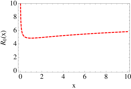
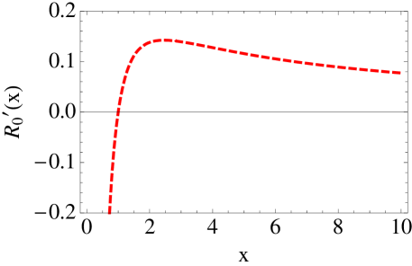
The function R0(x)subscript𝑅0𝑥R_{0}(x) and its derivative are shown in Fig. 1, we note that R0(1)=3g0/π2subscript𝑅013subscript𝑔0superscript𝜋2R_{0}(1)=3g_{0}/\pi^{2} and, as expected, R0(1)=0superscriptsubscript𝑅010R_{0}^{\prime}(1)=0.

Refer to caption
Refer to caption
Figure 1: Function R0(x)subscript𝑅0𝑥R_{0}(x) defined by Eq. (34) (upper part) and its derivative R0(x)superscriptsubscript𝑅0𝑥R_{0}^{\prime}(x) (lower part).

5.2 Anisotropic Bose-Einstein distribution

The function (28) may be considered as a Boltzmann equilibrium distribution that has been stretched (or squeezed) in the longitudinal direction. It is interesting to consider, in the similar way, the stretched (or squeezed) Bose-Einstein distribution,

fBE=g0exp(p2/λ2+p2/λ2)1.subscript𝑓𝐵𝐸subscript𝑔0superscriptsubscript𝑝perpendicular-to2superscriptsubscript𝜆perpendicular-to2superscriptsubscript𝑝parallel-to2superscriptsubscript𝜆parallel-to21f_{BE}=\frac{g_{0}}{\exp\left(\sqrt{p_{\perp}^{2}/\lambda_{\perp}^{2}+p_{\parallel}^{2}/\lambda_{\parallel}^{2}}\,\right)-1}. (35)

The corresponding definition of the entropy density for bosons is [20]

σ=g0λ2λ2π2𝑑ξξ𝑑ξ[fBEg0lnfBEg0(1+fBEg0)ln(1+fBEg0)].𝜎subscript𝑔0superscriptsubscript𝜆perpendicular-to2subscript𝜆parallel-to2superscript𝜋2differential-dsubscript𝜉perpendicular-tosubscript𝜉perpendicular-todifferential-dsubscript𝜉parallel-todelimited-[]subscript𝑓𝐵𝐸subscript𝑔0subscript𝑓𝐵𝐸subscript𝑔01subscript𝑓𝐵𝐸subscript𝑔01subscript𝑓𝐵𝐸subscript𝑔0\displaystyle\sigma=-\frac{g_{0}\lambda_{\perp}^{2}\,\lambda_{\parallel}}{2\pi^{2}}\int d\xi_{\perp}\,\xi_{\perp}\,d\xi_{\parallel}\,\left[\frac{f_{BE}}{g_{0}}\ln\frac{f_{BE}}{g_{0}}-\left(1+\frac{f_{BE}}{g_{0}}\right)\ln\left(1+\frac{f_{BE}}{g_{0}}\right)\right].
(36)

In this case the connection between the entropy density and the particle density is the same as in the isotropic gas of massless bosons,

σ=2π445ζ(3)n.𝜎2superscript𝜋445𝜁3𝑛\sigma=\frac{2\pi^{4}}{45\zeta(3)}\,n. (37)

Substituting Eq. (35) into Eqs. (23) and (24) we find, see Sect. 13,

gBE=ζ(3)g0π2,subscript𝑔𝐵𝐸𝜁3subscript𝑔0superscript𝜋2g_{BE}=\zeta(3)\frac{g_{0}}{\pi^{2}}, (38)
RBE(x)=ζ(4)R0(x)=π490R0(x).subscript𝑅𝐵𝐸𝑥𝜁4subscript𝑅0𝑥superscript𝜋490subscript𝑅0𝑥R_{BE}(x)=\zeta(4)\,R_{0}(x)=\frac{\pi^{4}}{90}R_{0}(x). (39)

Thus, for quantum statistics we obtain

ε(x,σ)𝜀𝑥𝜎\displaystyle\varepsilon(x,\sigma) =\displaystyle= (45ζ3/4(4)σ2π2g0)4/3R0(x),superscript45superscript𝜁344𝜎2superscript𝜋2subscript𝑔043subscript𝑅0𝑥\displaystyle\left(\frac{45\,\zeta^{3/4}(4)\,\sigma}{2\pi^{2}g_{0}}\right)^{4/3}R_{0}(x), (40)
P(x,σ)subscript𝑃perpendicular-to𝑥𝜎\displaystyle P_{\perp}(x,\sigma) =\displaystyle= (45ζ3/4(4)σ2π2g0)4/3[R0(x)3+xR0(x)],superscript45superscript𝜁344𝜎2superscript𝜋2subscript𝑔043delimited-[]subscript𝑅0𝑥3𝑥superscriptsubscript𝑅0𝑥\displaystyle\left(\frac{45\,\zeta^{3/4}(4)\,\sigma}{2\pi^{2}g_{0}}\right)^{4/3}\left[\frac{R_{0}(x)}{3}+xR_{0}^{\prime}(x)\right], (41)
P(x,σ)subscript𝑃parallel-to𝑥𝜎\displaystyle P_{\parallel}(x,\sigma) =\displaystyle= (45ζ3/4(4)σ2π2g0)4/3[R0(x)32xR0(x)].superscript45superscript𝜁344𝜎2superscript𝜋2subscript𝑔043delimited-[]subscript𝑅0𝑥32𝑥superscriptsubscript𝑅0𝑥\displaystyle\left(\frac{45\,\zeta^{3/4}(4)\,\sigma}{2\pi^{2}g_{0}}\right)^{4/3}\left[\frac{R_{0}(x)}{3}-2xR_{0}^{\prime}(x)\right]. (42)

We note that the numerical factor 45ζ3/4(4)/(2π2)2.4245superscript𝜁3442superscript𝜋22.4245\,\zeta^{3/4}(4)/(2\pi^{2})\approx 2.42 appearing in Eqs. (40)–(42) is very close to the factor π2/42.47superscript𝜋242.47\pi^{2}/4\approx 2.47 appearing in Eqs. (31)–(33), hence, the equations defining the energy density and pressures in terms of the entropy density and x𝑥x for the classical and quantum systems are practically the same.

6 One-dimensional boost-invariant motion

In the case of the longitudinal and boost-invariant evolution, the four-vectors Uμsuperscript𝑈𝜇U^{\mu} and Vμsuperscript𝑉𝜇V^{\mu} may be defined by the expressions

Uμ=(coshη,0,0,sinhη),superscript𝑈𝜇𝜂00𝜂\displaystyle U^{\mu}=(\cosh\eta,0,0,\sinh\eta), (43)
Vμ=(sinhη,0,0,coshη),superscript𝑉𝜇𝜂00𝜂\displaystyle V^{\mu}=(\sinh\eta,0,0,\cosh\eta), (44)

where η𝜂\eta is the space-time rapidity,

η=12lnt+ztz.𝜂12𝑡𝑧𝑡𝑧\displaystyle\eta=\frac{1}{2}\ln\frac{t+z}{t-z}. (45)

Substituting Eqs. (43) and (44) in Eqs. (9) and (10) we obtain

dεdτ=ε+Pτ,𝑑𝜀𝑑𝜏𝜀subscript𝑃parallel-to𝜏\displaystyle\frac{d\varepsilon}{d\tau}=-\frac{\varepsilon+P_{\parallel}}{\tau}, (46)
dσdτ+στ=Σ,𝑑𝜎𝑑𝜏𝜎𝜏Σ\displaystyle\frac{d\sigma}{d\tau}+\frac{\sigma}{\tau}=\Sigma, (47)

where τ𝜏\tau is the proper time

τ=t2z2.𝜏superscript𝑡2superscript𝑧2\tau=\sqrt{t^{2}-z^{2}}. (48)

6.1 Standard formulation

Substituting Eqs. (31) and (33) in (46), and using Eq. (25) for the entropy source, we obtain one ordinary differential equation for x𝑥x,

dxdτ=2xτ4H0(x)3τeq.𝑑𝑥𝑑𝜏2𝑥𝜏4subscript𝐻0𝑥3subscript𝜏eq\frac{dx}{d\tau}=\frac{2x}{\tau}-\frac{4H_{0}(x)}{3\tau_{\rm eq}}. (49)

We have introduced here the function H0(x)subscript𝐻0𝑥H_{0}(x) defined by the expression

H0(x)=R0(x)R0(x)Σστeq=R0(x)R0(x)(1x)2x.subscript𝐻0𝑥subscript𝑅0𝑥superscriptsubscript𝑅0𝑥Σ𝜎subscript𝜏eqsubscript𝑅0𝑥superscriptsubscript𝑅0𝑥superscript1𝑥2𝑥\displaystyle H_{0}(x)=\frac{R_{0}(x)}{R_{0}^{\prime}(x)}\frac{\Sigma}{\sigma}\tau_{\rm eq}=\frac{R_{0}(x)}{R_{0}^{\prime}(x)}\frac{(1-\sqrt{x})^{2}}{\sqrt{x}}. (50)

For small deviations from equilibrium we may use the expansion

H0(x)4516(x1)+195112(x1)2+.subscript𝐻0𝑥4516𝑥1195112superscript𝑥12\displaystyle H_{0}(x)\approx\frac{45}{16}(x-1)+\frac{195}{112}(x-1)^{2}+\cdots. (51)

Equation (49) was analyzed in detail in Ref. [1], where we showed that x1𝑥1x\to 1 for ττeqmuch-greater-than𝜏subscript𝜏eq\tau\gg\tau_{\rm eq}.

6.2 Modified entropy source

Let us now turn to the discussion of the entropy source defined by the difference of pressures. If we use Eq. (27) instead of Eq. (25), we obtain

dxdτ=2xτ4H~(x)3τ~eq,𝑑𝑥𝑑𝜏2𝑥𝜏4~𝐻𝑥3subscript~𝜏eq\frac{dx}{d\tau}=\frac{2x}{\tau}-\frac{4{\tilde{H}}(x)}{3{\tilde{\tau}}_{\rm eq}}, (52)

where

H~(x)=9x2R0(x)R0(x)(R0(x)/3+xR0(x))(R0(x)/32xR0(x)).~𝐻𝑥9superscript𝑥2subscript𝑅0𝑥superscriptsubscript𝑅0𝑥subscript𝑅0𝑥3𝑥superscriptsubscript𝑅0𝑥subscript𝑅0𝑥32𝑥superscriptsubscript𝑅0𝑥\displaystyle{\tilde{H}}(x)=\frac{9x^{2}R_{0}(x)R_{0}^{\prime}(x)}{\left(R_{0}(x)/3+xR_{0}^{\prime}(x)\right)\left(R_{0}(x)/3-2xR_{0}^{\prime}(x)\right)}. (53)

Similarly to (51) we may expand (53) around x=1𝑥1x=1,

H~(x)365(x1)+816175(x1)2+.~𝐻𝑥365𝑥1816175superscript𝑥12\displaystyle\tilde{H}(x)\approx\frac{36}{5}(x-1)+\frac{816}{175}(x-1)^{2}+\cdots. (54)

The requirement that the two definitions of the entropy source lead to the same behavior in the region close to equilibrium leads to the condition

τ~eq=6425τeq.subscript~𝜏eq6425subscript𝜏eq{\tilde{\tau}}_{\rm eq}=\frac{64}{25}\,{\tau}_{\rm eq}. (55)
Refer to caption
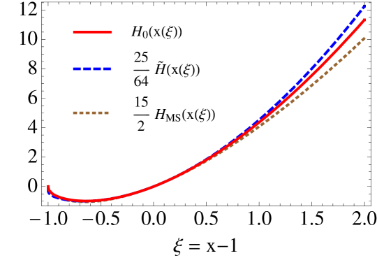
Figure 2: Function H0subscript𝐻0H_{0} defined by Eq. (50) (solid line) compared to the rescaled functions H~~𝐻{\tilde{H}} and HMSsubscript𝐻MSH_{{\rm MS}} defined by Eqs. (53) and (60) (dashed and dotted lines, respectively). The arguments of the functions have been shifted to ξ=x1𝜉𝑥1\xi=x-1.
Refer to caption
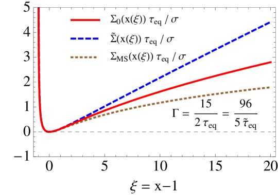
Figure 3: Different entropy source terms normalized by σ/τeq𝜎subscript𝜏eq\sigma/\tau_{\rm eq}. The relaxation times are connected by the formula (62).

6.3 Martinez and Strickland model

A similar model to ADHYDRO has been introduced recently by Martinez and Strickland (MS) [12, 13]. This model is based on the consideration of the two first moment of the Boltzmann kinetic equation with the collision term treated in the relaxation time approximation. The inverse of the relaxation time is denoted by ΓΓ\Gamma.

In this approach the evolution of matter is described by two coupled ordinary differential equations for the momentum anisotropy ξ𝜉\xi and the typical hard momentum scale phardsubscript𝑝hardp_{\rm hard}. They may be written in the compact form as

dξdτ=2(1+ξ)τ4ΓHMS(ξ)3,𝑑𝜉𝑑𝜏21𝜉𝜏4Γsubscript𝐻MS𝜉3\displaystyle\frac{d\xi}{d\tau}=\frac{2(1+\xi)}{\tau}-\frac{4\Gamma H_{{\rm MS}}(\xi)}{3}, (56)
1pharddpharddτ=Γ3RMS(ξ)RMS(ξ)HMS(ξ).1subscript𝑝hard𝑑subscript𝑝hard𝑑𝜏Γ3subscriptsuperscript𝑅MS𝜉subscript𝑅MS𝜉subscript𝐻MS𝜉\displaystyle\frac{1}{p_{\rm hard}}\frac{dp_{\rm hard}}{d\tau}=\frac{\Gamma}{3}\frac{R^{\prime}_{{\rm MS}}(\xi)}{R_{{\rm MS}}(\xi)}H_{{\rm MS}}(\xi). (57)

The parameter ξ𝜉\xi is related to x𝑥x,

ξ=x1.𝜉𝑥1\xi=x-1. (58)

Similarly, the function RMS(ξ)subscript𝑅MS𝜉R_{{\rm MS}}(\xi) is simply connected to R0(x)subscript𝑅0𝑥R_{0}(x),

RMS(ξ)=12[11+ξ+arctanξξ]=π23g0(1+ξ)2/3R0(1+ξ).subscript𝑅MS𝜉12delimited-[]11𝜉𝜉𝜉superscript𝜋23subscript𝑔0superscript1𝜉23subscript𝑅01𝜉\displaystyle R_{{\rm MS}}(\xi)=\frac{1}{2}\left[\frac{1}{1+\xi}+\frac{\arctan\sqrt{\xi}}{\sqrt{\xi}}\right]=\frac{\pi^{2}}{3g_{0}}(1+\xi)^{-2/3}R_{0}(1+\xi). (59)

In order to show similarities with our approach, in Eqs. (56) and (57) we have introduced the function HMSsubscript𝐻MSH_{{\rm MS}} that is an analog of H0(x)subscript𝐻0𝑥H_{0}(x),

HMS(ξ)=3(ξ+1)(ξ+1RMS3/4(ξ)1)RMS(ξ)2RMS(ξ)+3(ξ+1)RMS(ξ).subscript𝐻MS𝜉3𝜉1𝜉1superscriptsubscript𝑅MS34𝜉1subscript𝑅MS𝜉2subscript𝑅MS𝜉3𝜉1superscriptsubscript𝑅MS𝜉\displaystyle H_{{\rm MS}}(\xi)=\frac{3(\xi+1)\left(\sqrt{\xi+1}R_{{\rm MS}}^{3/4}(\xi)-1\right)R_{{\rm MS}}(\xi)}{2R_{{\rm MS}}(\xi)+3(\xi+1)R_{{\rm MS}}^{\prime}(\xi)}. (60)

Close to equilibrium, the function HMS(ξ(x))subscript𝐻MS𝜉𝑥H_{{\rm MS}}(\xi(x)) has the following expansion

HMS(ξ(x))38(x1)+1784(x1)2+.subscript𝐻MS𝜉𝑥38𝑥11784superscript𝑥12\displaystyle H_{{\rm MS}}(\xi(x))\approx\frac{3}{8}(x-1)+\frac{17}{84}(x-1)^{2}+\cdots. (61)

Thus, comparing Eqs. (49) and (56) we conclude that our standard approach is equivalent to MS (near equilibrium) if

Γ=152τeq=965τ~eq.Γ152subscript𝜏eq965subscript~𝜏eq\Gamma=\frac{15}{2\tau_{\rm eq}}=\frac{96}{5{\tilde{\tau}}_{\rm eq}}. (62)

The plots of the functions H0(x(ξ))subscript𝐻0𝑥𝜉H_{0}(x(\xi)), H~(x(ξ))~𝐻𝑥𝜉{\tilde{H}}(x(\xi)) and HMS(x(ξ))subscript𝐻MS𝑥𝜉H_{{\rm MS}}(x(\xi)), rescaled by the factors defined in (62), are shown in Fig. 2. As it has been already discussed in [2] the essential difference between these functions is observed only for very large anisotropies.

It is instructive to identify the entropy source in the Martinez and Strickland model. The entropy density in this model has the form σ=Aphard3x1/2𝜎𝐴superscriptsubscript𝑝hard3superscript𝑥12\sigma=Ap_{\rm hard}^{3}x^{-1/2}. With the help of Eqs. (56) and (57) we reproduce Eq. (47) with

Σ=ΣMSΣsubscriptΣMS\displaystyle\Sigma=\Sigma_{{\rm MS}} =\displaystyle= σΓ[RMS(ξ)RMS(ξ)+23(1+ξ)]HMS(ξ)𝜎Γdelimited-[]subscriptsuperscript𝑅MS𝜉subscript𝑅MS𝜉231𝜉subscript𝐻MS𝜉\displaystyle\sigma\Gamma\left[\frac{R^{\prime}_{{\rm MS}}(\xi)}{R_{{\rm MS}}(\xi)}+\frac{2}{3(1+\xi)}\right]H_{{\rm MS}}(\xi) (63)
=\displaystyle= σΓR0(x)R0(x)HMS(ξ(x)).𝜎Γsuperscriptsubscript𝑅0𝑥subscript𝑅0𝑥subscript𝐻MS𝜉𝑥\displaystyle\sigma\Gamma\,\frac{R_{0}^{\prime}(x)}{R_{0}(x)}\,H_{{\rm MS}}(\xi(x)).

Thus, comparing Eqs. (50) and (63) we find that the Martinez and Strickland model fits exactly to the ADHYDRO scheme if the entropy source is defined by (63).

Moreover, expanding functions RMS(ξ)subscript𝑅MS𝜉R_{{\rm MS}}(\xi) and HMS(ξ)subscript𝐻MS𝜉H_{{\rm MS}}(\xi) for small ξ𝜉\xi, and using Eq. (62), we find that ΣMSsubscriptΣMS\Sigma_{{\rm MS}} agrees with Σ0subscriptΣ0\Sigma_{0} and Σ~~Σ{\tilde{\Sigma}} up to quadratic terms in ξ𝜉\xi. Different entropy source terms normalized by σ/τeq𝜎subscript𝜏eq\sigma/\tau_{\rm eq} are shown in Fig. 3. Once again, the relaxation times are identified with the help of Eq. (62).
Refer to caption
Refer to caption
Refer to caption
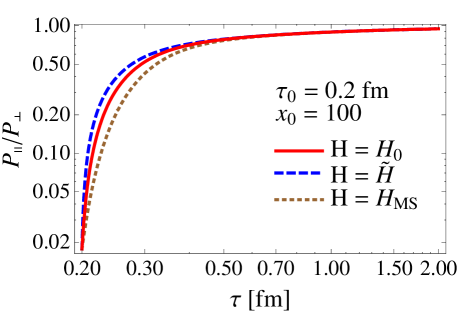
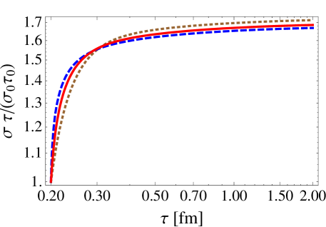
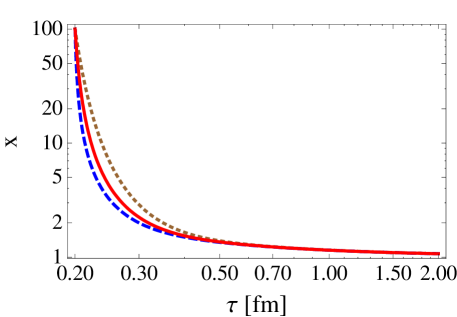
Figure 4: Time dependence of the asymmetry parameter x𝑥x (upper part), ratio of the longitudinal and transverse pressures (middle part), and entropy density normalized to the values obtained from the Bjorken model, σBj=σ0τ0/τsubscript𝜎Bjsubscript𝜎0subscript𝜏0𝜏\sigma_{\rm Bj}=\sigma_{0}\tau_{0}/\tau (lower part). The standard ADHYDRO calculations are shown as solid lines, the results of ADHYDRO with the modified entropy source are represented by dashed lines, and the results for the MS model are shown as dotted lines.

7 Results for the boost-invariant case

In this Section we present numerical solutions of Eqs. (49), (52) and (56). As discussed above, these equations correspond to three different forms of the entropy source defined by Eqs. (25), (27), and (63), respectively. The parameter τeqsubscript𝜏eq\tau_{\rm eq} is set equal to 0.250.250.25 fm. Using this value we find that the system equilibrates at the proper time of about 1 fm. The values of the time-scale parameter τ~eqsubscript~𝜏eq{\tilde{\tau}_{\rm eq}} and the inverse relaxation time ΓΓ\Gamma are connected with τeqsubscript𝜏eq\tau_{\rm eq} by Eq. (62).

In all the cases the initial conditions are specified at the initial proper time τ0=0.2subscript𝜏00.2\tau_{0}=0.2 fm. We assume that the transverse pressure dominates over the longitudinal pressure during the very early stages of the evolution of matter and take x(τ0)=x0=100𝑥subscript𝜏0subscript𝑥0100x(\tau_{0})=x_{0}=100. In the upper part of Fig. 4 we show the time dependence of x𝑥x. The solid line describes the standard ADHYDRO result, with Σ=Σ0ΣsubscriptΣ0\Sigma=\Sigma_{0}, the dashed line describes the result obtained with the modified entropy source in ADHYDRO, with Σ=Σ~Σ~Σ\Sigma={\tilde{\Sigma}}, and the dotted line describes the time evolution of x𝑥x in the MS model where Σ=ΣMSΣsubscriptΣMS\Sigma=\Sigma_{{\rm MS}}.

The middle part of Fig. 4 shows the time evolution of the ratio of the longitudinal and transverse pressure, and the lower part of Fig. 4 shows the time evolution of the entropy density normalized to the initial entropy density. The notation is the same as in the upper part of Fig. 4.

We observe that the time dependence of x𝑥x is very much similar in the three cases, suggesting that the particular form of the entropy source has small effect on the time evolution (note the double logarithmic scale). This behavior is caused by the initial large entropy production that leads to a fast decrease of x𝑥x. Later, when x𝑥x becomes closer to unity, all the schemes are equivalent and imply a very similar time development.

We find, however, that the equilibration of pressures is a little bit delayed in the MS model, as compared to the standard version, and this is reflected in a larger entropy production (relative to the initial entropy density). On the other hand, the equilibration in the modified model where Σ=Σ~Σ~Σ\Sigma={\tilde{\Sigma}} is a little bit accelerated.

8 Non-boost-invariant evolution

In the case of purely one-dimensional, non-boost-invariant motion we define

Uμ=(coshϑ(τ,η),0,0,sinhϑ(τ,η)),superscript𝑈𝜇italic-ϑ𝜏𝜂00italic-ϑ𝜏𝜂\displaystyle U^{\mu}=\left(\cosh\vartheta(\tau,\eta),0,0,\sinh\vartheta(\tau,\eta)\right), (64)
Vμ=(sinhϑ(τ,η),0,0,coshϑ(τ,η)),superscript𝑉𝜇italic-ϑ𝜏𝜂00italic-ϑ𝜏𝜂\displaystyle V^{\mu}=\left(\sinh\vartheta(\tau,\eta),0,0,\cosh\vartheta(\tau,\eta)\right), (65)

where ϑ(τ,η)italic-ϑ𝜏𝜂\vartheta(\tau,\eta) is the fluid rapidity which depends on proper time and space-time rapidity. Equations (64) and (65) guarantee that Eqs. (4) are automatically satisfied.

Using Eqs. (64) and (65) in Eqs. (9) and (10) we derive three partial differential equations for σ(τ,η)𝜎𝜏𝜂\sigma(\tau,\eta), ϑ(τ,η)italic-ϑ𝜏𝜂\vartheta(\tau,\eta), and x(τ,η)𝑥𝜏𝜂x(\tau,\eta). The structure of those equations has been discussed recently in Ref. [2] and in this paper we skip details describing their derivation and form. It is important, however, to present here our initial conditions.
Refer to caption
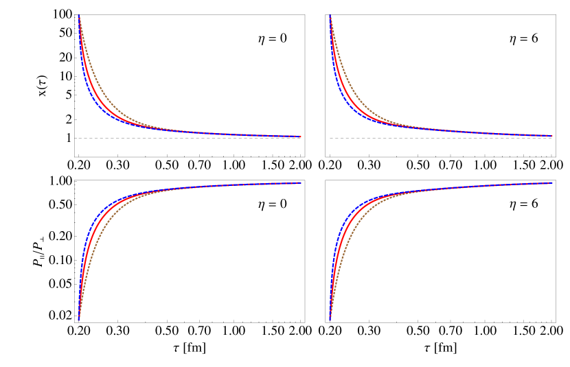
Figure 5: Upper parts: time evolution of the anisotropy parameter x𝑥x for two different values of the space-time rapidity η=0𝜂0\eta=0 (left) and η=6𝜂6\eta=6 (right). Lower parts: time dependence of the ratio of the longitudinal and transverse pressures, P/Psubscript𝑃parallel-tosubscript𝑃perpendicular-toP_{\parallel}/P_{\perp}, again for η=0𝜂0\eta=0 (left) and η=6𝜂6\eta=6 (right). The solid lines represent the standard calculation where Σ=Σ0ΣsubscriptΣ0\Sigma=\Sigma_{0}, the dashed lines show the results with the modified entropy source where Σ=Σ~Σ~Σ\Sigma={\tilde{\Sigma}}, and the dotted lines show the results for Σ=ΣMSΣsubscriptΣMS\Sigma=\Sigma_{{\rm MS}}.
Refer to caption
Refer to caption
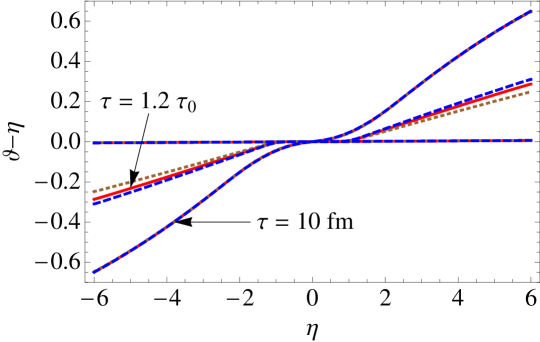
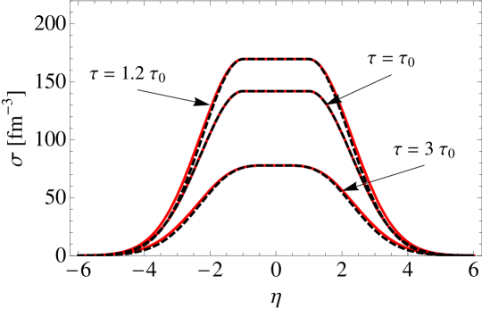
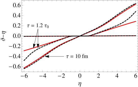
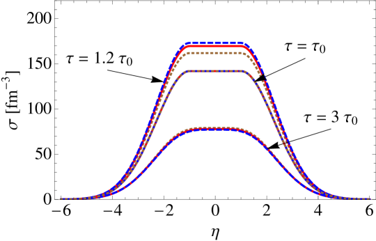
Figure 6: Time evolution of the entropy (upper part) and fluid rapidity (lower part) profiles in η𝜂\eta. Similarly as in Fig. 5, the solid, dashed, and dotted lines correspond to three different forms of the entropy source used in the numerical calculations.

The initial conditions for a non-boost-invariant evolution are defined by the three functions of space-time rapidity: σ(τ0,η)𝜎subscript𝜏0𝜂\sigma(\tau_{0},\eta), ϑ(τ0,η)italic-ϑsubscript𝜏0𝜂\vartheta(\tau_{0},\eta), and x(τ0,η)𝑥subscript𝜏0𝜂x(\tau_{0},\eta). The initial entropy profile is taken in the form [11, 21]

σ(τ0,η)=σ0exp[(|η|Δη)22(δη)2θ(|η|Δη)],𝜎subscript𝜏0𝜂subscript𝜎0superscript𝜂Δ𝜂22superscript𝛿𝜂2𝜃𝜂Δ𝜂\displaystyle\sigma(\tau_{0},\eta)=\sigma_{0}\exp\left[-\frac{(|\eta|-\Delta\eta)^{2}}{2(\delta\eta)^{2}}\;\theta(|\eta|-\Delta\eta)\right], (66)

where θ𝜃\theta is the step function, the parameter ΔηΔ𝜂\Delta\eta defines the half width of the initial plateau in space-time rapidity, and δη𝛿𝜂\delta\eta defines the half width of the Gaussian tails on both sides of the plateau. To match the rapidity distribution measured by BRAHMS [22] we use the values: Δη=1Δ𝜂1\Delta\eta=1 and δη=1.3𝛿𝜂1.3\delta\eta=1.3. The value of the initial central entropy density is obtained from the condition that the initial energy density is 100 GeV/fm3,

ε0=100GeV/fm3=(π2σ04g0)4/3R(x0).subscript𝜀0100GeV/fm3superscriptsuperscript𝜋2subscript𝜎04subscript𝑔043𝑅subscript𝑥0\varepsilon_{0}=100\,\hbox{GeV/fm${}^{3}$}=\left(\frac{\pi^{2}\sigma_{0}}{4g_{0}}\right)^{4/3}R(x_{0}). (67)

Here, x0subscript𝑥0x_{0} is the initial value of the anisotropy parameter at η=0𝜂0\eta=0. In this Section we assume that the initial profile of x𝑥x is constant,

x(τ0,η)=x0=100.𝑥subscript𝜏0𝜂subscript𝑥0100x(\tau_{0},\eta)=x_{0}=100. (68)

The time-scale parameter τeqsubscript𝜏eq\tau_{\rm eq} has the same value as in the previous Section, and the initial fluid rapidity profile is taken in the form

ϑ(τ0,η)=η.italic-ϑsubscript𝜏0𝜂𝜂\vartheta(\tau_{0},\eta)=\eta. (69)

The results of our numerical calculations done with three different forms of the entropy source are shown in Figs. 5 and 6. The solid lines represent the standard calculation where Σ=Σ0ΣsubscriptΣ0\Sigma=\Sigma_{0}, the dashed lines show the results with the modified entropy source where Σ=Σ~Σ~Σ\Sigma={\tilde{\Sigma}}, and the dotted lines show the results for the case Σ=ΣMSΣsubscriptΣMS\Sigma=\Sigma_{{\rm MS}}. In the two upper parts of Fig. 5 we show the time dependence of the anisotropy parameter x𝑥x for two different values of the space-time rapidity, η=0𝜂0\eta=0 (left) and η=6𝜂6\eta=6 (right). We observe that this dependence is very much similar to the dependence obtained in the boost-invariant calculation, see the upper part of Fig. 4. Thus the rapidity dependence of the initial entropy profile does not affect the time dependence of x𝑥x in a noticeable way. In the two lower parts of Fig. 5 we show the time dependence of the ratio of pressures, P/Psubscript𝑃parallel-tosubscript𝑃perpendicular-toP_{\parallel}/P_{\perp}. Again, we observe weak rapidity dependence, compare the middle part of Fig. 4.

In Fig. 6 we show the entropy density σ𝜎\sigma and the fluid rapidity ϑitalic-ϑ\vartheta as functions of space-time rapidity for the initial proper time τ=τ0𝜏subscript𝜏0\tau=\tau_{0}, a bit later proper time τ=1.2τ0𝜏1.2subscript𝜏0\tau=1.2\,\tau_{0}, and τ=3τ0𝜏3subscript𝜏0\tau=3\,\tau_{0} (for σ𝜎\sigma) or τ=10𝜏10\tau=10 fm (for ϑηitalic-ϑ𝜂\vartheta-\eta). At τ=1.2τ0𝜏1.2subscript𝜏0\tau=1.2\,\tau_{0} the entropy profiles are higher than the initial profiles — at such an early time the entropy is produced in the system. For τ=3τ0𝜏3subscript𝜏0\tau=3\,\tau_{0} the entropy profiles lie below the initial profiles — the entropy is not produced in the system anymore, and the entropy density drops due to the longitudinal expansion of the system. We observe that the results obtained with the three forms of ΣΣ\Sigma are very much similar, indicating that the specific form of the entropy form has small effect on the evolution of matter also for the non-boost-invariant systems.

Refer to caption
Refer to caption
Figure 7: Time evolution of the anisotropy parameter x𝑥x (upper part) and the ratio of pressures (lower part) for three different values of the space-time rapidity: η=0𝜂0\eta=0 (solid lines), η=4.9𝜂4.9\eta=4.9 (dashed lines), and η=6𝜂6\eta=6 (dotted lines).

9 Rapidity dependent anisotropy

In the previous Section we have analyzed the case where the initial anisotropy parameter is independent of space-time rapidity, x(τ0,η)=x0𝑥subscript𝜏0𝜂subscript𝑥0x(\tau_{0},\eta)=x_{0}. In this Section we consider the case where the initial anisotropy profile depends on η𝜂\eta but other initial conditions are exactly the same. We assume that the initial η𝜂\eta profile of x𝑥x is the same as the initial entropy density profile, namely

x(τ0,η)=x0σ(τ0,η)σ0,𝑥subscript𝜏0𝜂subscript𝑥0𝜎subscript𝜏0𝜂subscript𝜎0\displaystyle x(\tau_{0},\eta)=x_{0}\frac{\sigma(\tau_{0},\eta)}{\sigma_{0}}, (70)

where σ(τ0,η)𝜎subscript𝜏0𝜂\sigma(\tau_{0},\eta) is given by Eq. (66). With x0=100subscript𝑥0100x_{0}=100 Eq. (70) implies that the initial anisotropy is large at the center of the system (central region) and small at the edges of the system (fragmentation regions).

In Fig. 7 we show the time evolution of the anisotropy parameter x𝑥x and the ratio of pressures for three different values of the space-time rapidity: η=0𝜂0\eta=0 (solid lines), η=4.9𝜂4.9\eta=4.9 (dashed lines), and η=6𝜂6\eta=6 (dotted lines). The behavior of the system in the central region (η=0𝜂0\eta=0) is very much similar to the behavior of the boost-invariant systems studied before. On the other hand, at large rapidities the time evolution of the physical quantities is quite different, which is caused by a different starting value of x𝑥x. For small initial values of x𝑥x we observe first the growth of x𝑥x with time (above unity) and only later a decrease towards unity. Anyway, we observe that at τ0.5𝜏0.5\tau\approx 0.5 fm the values of x𝑥x become practically independent of η𝜂\eta.

Refer to caption
Refer to caption
Figure 8: Time evolution of the entropy and rapidity profiles for the initial conditions specified by Eqs. (66), (68), and (69) (solid lines) and by Eqs. (66), (69) and (70) (dashed lines).

In Fig. 8 we show the time evolution of the entropy and rapidity profiles for the initial conditions specified by Eqs. (66), (68), and (69) (solid lines) and by Eqs. (66), (69) and (70) (dashed lines). In the two considered cases the entropy profiles behave in the very similar way. The behavior of the fluid rapidity is different only at the beginning of the evolution for large rapidities.

10 Conclusions

In this paper we have discussed the assumptions of the recently formulated model that may be used to describe the evolution of a highly-anisotropic fluid formed at the very early stages of relativistic heavy-ion collisions. We have considered three forms of the entropy source which defines the dynamics of the system. We have found that the numerical results depend very weakly on the particular form of the entropy source.

We have also studied microscopic interpretation of the model, discussing different forms of the microscopic phase-space distribution function. We have found that corrections for quantum effects lead to minor quantitative differences as compared to the standard case where the phase space distribution is described by the (stretched or squeezed) Boltzmann distribution.

We have performed the numerical calculations for the cases where the initial anisotropy depends on space-time rapidity. In such cases the evolution of the system is more complicated but the tendency of the system to equilibrate is not changed.

Altogether, we have found that the results obtained with the ADHYDRO model are stable against various modifications of the model components such as: the entropy source, the form of the microscopic phase-space distribution function, or the form of the initial conditions. We consider such stability as an attractive physical feature of the model proposed in [1].

11 Appendix 1

In this Section we give the explicit form of the Lorentz transformation which leads from the center-of-mass frame of the colliding nuclei to the local-rest-frame of the fluid element. This transformation is constructed as a sequence of the longitudinal Lorentz boost, rotation around the z𝑧z-axis, and the transverse Lorentz boost. In this way the complete transformation does not change the longitudinal direction.

The four-vectors Uμsuperscript𝑈𝜇U^{\mu} and Vμsuperscript𝑉𝜇V^{\mu} may be written in the following form

Uμsuperscript𝑈𝜇\displaystyle U^{\mu} =\displaystyle= coshϑcoshϑ(1,tanhϑcosϕcoshϑ,tanhϑcosϕcoshϑ,tanhϑ),subscriptitalic-ϑparallel-tosubscriptitalic-ϑperpendicular-to1subscriptitalic-ϑperpendicular-toitalic-ϕsubscriptitalic-ϑparallel-tosubscriptitalic-ϑperpendicular-toitalic-ϕsubscriptitalic-ϑparallel-tosubscriptitalic-ϑparallel-to\displaystyle\cosh\vartheta_{\parallel}\cosh\vartheta_{\perp}\left(1,\frac{\tanh\vartheta_{\perp}\cos\phi}{\cosh\vartheta_{\parallel}},\frac{\tanh\vartheta_{\perp}\cos\phi}{\cosh\vartheta_{\parallel}},\tanh\vartheta_{\parallel}\right),
Vμsuperscript𝑉𝜇\displaystyle V^{\mu} =\displaystyle= coshϑ(tanhϑ,0,0,1).subscriptitalic-ϑparallel-tosubscriptitalic-ϑparallel-to001\displaystyle\cosh\vartheta_{\parallel}\left(\tanh\vartheta_{\parallel},0,0,1\right). (71)

where ϑsubscriptitalic-ϑparallel-to\vartheta_{\parallel} is the longitudinal fluid rapidity and ϑsubscriptitalic-ϑperpendicular-to\vartheta_{\perp} is the transverse fluid rapidity.

The Lorentz transformation leading to the local rest frame consists of the Lorentz boost along the z𝑧z-axis,

L(z)νμ=(coshϑ00sinhϑ01000010sinhϑ00coshϑ),subscriptsuperscript𝐿𝜇𝑧𝜈subscriptitalic-ϑparallel-to00subscriptitalic-ϑparallel-to01000010subscriptitalic-ϑparallel-to00subscriptitalic-ϑparallel-toL^{\,\mu}_{(z)\,\nu}=\left(\begin{array}[]{cccc}\cosh\vartheta_{\parallel}&0&0&-\sinh\vartheta_{\parallel}\\ 0&1&0&0\\ 0&0&1&0\\ -\sinh\vartheta_{\parallel}&0&0&\cosh\vartheta_{\parallel}\end{array}\right), (72)

the rotation around the z𝑧z-axis,

R(xy)νμ=(10000cosϕsinϕ00sinϕcosϕ00001),subscriptsuperscript𝑅𝜇𝑥𝑦𝜈10000italic-ϕitalic-ϕ00italic-ϕitalic-ϕ00001R^{\,\mu}_{(xy)\,\nu}=\left(\begin{array}[]{cccc}1&0&0&0\\ 0&\cos\phi&\sin\phi&0\\ 0&-\sin\phi&\cos\phi&0\\ 0&0&0&1\end{array}\right), (73)

and the Lorentz boost along the x𝑥x-axis

L(x)νμ=(coshϑsinhϑ00sinhϑcoshϑ0000100001).subscriptsuperscript𝐿𝜇𝑥𝜈subscriptitalic-ϑperpendicular-tosubscriptitalic-ϑperpendicular-to00subscriptitalic-ϑperpendicular-tosubscriptitalic-ϑperpendicular-to0000100001L^{\,\mu}_{(x)\,\nu}=\left(\begin{array}[]{cccc}\cosh\vartheta_{\perp}&-\sinh\vartheta_{\perp}&0&0\\ -\sinh\vartheta_{\perp}&\cosh\vartheta_{\perp}&0&0\\ 0&0&1&0\\ 0&0&0&1\end{array}\right). (74)

By direct multiplication one may check that

L(x)βαR(xy)γβL(z)μγUμsubscriptsuperscript𝐿𝛼𝑥𝛽subscriptsuperscript𝑅𝛽𝑥𝑦𝛾subscriptsuperscript𝐿𝛾𝑧𝜇superscript𝑈𝜇\displaystyle L^{\,\alpha}_{(x)\,\beta}R^{\,\beta}_{(xy)\,\gamma}L^{\,\gamma}_{(z)\,\mu}U^{\mu} =\displaystyle= (1,0,0,0),1000\displaystyle(1,0,0,0),
L(x)βαR(xy)γβL(z)μγVμsubscriptsuperscript𝐿𝛼𝑥𝛽subscriptsuperscript𝑅𝛽𝑥𝑦𝛾subscriptsuperscript𝐿𝛾𝑧𝜇superscript𝑉𝜇\displaystyle L^{\,\alpha}_{(x)\,\beta}R^{\,\beta}_{(xy)\,\gamma}L^{\,\gamma}_{(z)\,\mu}V^{\mu} =\displaystyle= (0,0,0,1).0001\displaystyle(0,0,0,1). (75)

In order to move from the local rest frame to the center-of-mass frame we perform the inverse transormation.

12 Appendix 2

The concept of ADHYDRO includes, as a special case, the framework of transverse hydrodynamics. In the latter case, we assume that the distribution function (14) has the following factorized form

f𝑓\displaystyle f =\displaystyle= f((pU)2(pV)2λ)f(pVλ)=f(pUλ)n0τδ(pV).subscript𝑓perpendicular-tosuperscript𝑝𝑈2superscript𝑝𝑉2subscript𝜆perpendicular-tosubscript𝑓parallel-to𝑝𝑉subscript𝜆perpendicular-tosubscript𝑓perpendicular-to𝑝𝑈subscript𝜆perpendicular-tosubscript𝑛0𝜏𝛿𝑝𝑉\displaystyle f_{\perp}\left(\frac{\sqrt{(p\cdot U)^{2}-(p\cdot V)^{2}}}{\lambda_{\perp}}\right)f_{\parallel}\left(\frac{p\cdot V}{\lambda_{\perp}}\right)=f_{\perp}\left(\frac{p\cdot U}{\lambda_{\perp}}\right)\frac{n_{0}}{\tau}\delta\left(p\cdot V\right).

Here n0subscript𝑛0n_{0} is a normalization constant and δ𝛿\delta is the Dirac delta function. Equation (LABEL:TH1) allows us to make the identification

λ=1τ.subscript𝜆parallel-to1𝜏\lambda_{\parallel}=\frac{1}{\tau}. (77)

Using our general definition of the function R(x)𝑅𝑥R(x), see Eq. (23), we find

R(x)=rx1/6,xR(x)=R(x)6,formulae-sequence𝑅𝑥𝑟superscript𝑥16𝑥superscript𝑅𝑥𝑅𝑥6R(x)=rx^{1/6},\quad xR^{\prime}(x)=\frac{R(x)}{6}, (78)

where r𝑟r is a constant. Equations (78) used in (20)–(22) immediately yield

P=ε2,P=0.formulae-sequencesubscript𝑃perpendicular-to𝜀2subscript𝑃parallel-to0P_{\perp}=\frac{\varepsilon}{2},\quad P_{\parallel}=0. (79)

Hence, the ansatz (LABEL:TH1) corresponds to the situation where the longitudinal pressure vanishes and the system may be treated as a collection of independent clusters which expand transversally.

The parameter λsubscript𝜆perpendicular-to\lambda_{\perp} describes temperature of two-dimensional transverse clusters. For the purely longitudinal expansion, the parton density drops like 1/τ1𝜏1/\tau. Since nλ2λ=λ2/τsimilar-to𝑛superscriptsubscript𝜆perpendicular-to2subscript𝜆parallel-tosuperscriptsubscript𝜆perpendicular-to2𝜏n\sim\lambda_{\perp}^{2}\lambda_{\parallel}=\lambda_{\perp}^{2}/\tau, the value of λsubscript𝜆perpendicular-to\lambda_{\perp} remains unchanged. Clearly, only transverse expansion can lower cluster’s temperature. Moreover, in such a boost-invariant case xτ2similar-to𝑥superscript𝜏2x\sim\tau^{2}, hence the ratio of the transverse and longitudinal pressure always grows and the system cannot reach stable isotropic equilibrium.

13 Appendix 3

In this Appendix we discuss consequences of replacing the classical distribution function by its quantum analogs, the Bose-Einstein and Fermi-Dirac distributions. The integrals over the distribution function (35) may be done by expanding (35) in a geometric series,

fBE=g0n=1exp(np2/λ2+p2/λ2),subscript𝑓𝐵𝐸subscript𝑔0superscriptsubscript𝑛1𝑛superscriptsubscript𝑝perpendicular-to2superscriptsubscript𝜆perpendicular-to2superscriptsubscript𝑝parallel-to2superscriptsubscript𝜆parallel-to2f_{BE}=g_{0}\sum_{n=1}^{\infty}\exp\left(-n\sqrt{p_{\perp}^{2}/\lambda_{\perp}^{2}+p_{\parallel}^{2}/\lambda_{\parallel}^{2}}\,\right), (80)

and by integrating (80) term by term. For example, starting from the general definition of the function R(x)𝑅𝑥R(x), see Eq. (23), we obtain

RBE(x)subscript𝑅𝐵𝐸𝑥\displaystyle R_{BE}(x) =\displaystyle= g0x1/3n=1dξξdξ2π2ξ2+xξ2exp(nξ2+ξ2).subscript𝑔0superscript𝑥13superscriptsubscript𝑛1𝑑subscript𝜉perpendicular-tosubscript𝜉perpendicular-to𝑑subscript𝜉parallel-to2superscript𝜋2superscriptsubscript𝜉parallel-to2𝑥superscriptsubscript𝜉perpendicular-to2𝑛superscriptsubscript𝜉perpendicular-to2superscriptsubscript𝜉parallel-to2\displaystyle g_{0}x^{-1/3}\sum_{n=1}^{\infty}\int\frac{d\xi_{\perp}\xi_{\perp}d\xi_{\parallel}}{2\pi^{2}}\sqrt{\xi_{\parallel}^{2}+x\xi_{\perp}^{2}}\exp\left(-n\sqrt{\xi_{\perp}^{2}+\xi_{\parallel}^{2}}\,\right).

Introducing the new integration variables: x=nξsubscript𝑥perpendicular-to𝑛subscript𝜉perpendicular-tox_{\perp}=n\,\xi_{\perp} and x=nξsubscript𝑥parallel-to𝑛subscript𝜉parallel-tox_{\parallel}=n\,\xi_{\parallel} we find

RBE(x)subscript𝑅𝐵𝐸𝑥\displaystyle R_{BE}(x) =\displaystyle= g0x1/3n=11n4dxxdx2π2x2+xx2exp(x2+x2).subscript𝑔0superscript𝑥13superscriptsubscript𝑛11superscript𝑛4𝑑subscript𝑥perpendicular-tosubscript𝑥perpendicular-to𝑑subscript𝑥parallel-to2superscript𝜋2superscriptsubscript𝑥parallel-to2𝑥superscriptsubscript𝑥perpendicular-to2superscriptsubscript𝑥perpendicular-to2superscriptsubscript𝑥parallel-to2\displaystyle g_{0}x^{-1/3}\sum_{n=1}^{\infty}\frac{1}{n^{4}}\int\frac{dx_{\perp}x_{\perp}dx_{\parallel}}{2\pi^{2}}\sqrt{x_{\parallel}^{2}+xx_{\perp}^{2}}\exp\left(-\sqrt{x_{\perp}^{2}+x_{\parallel}^{2}}\,\right).

The sum over n𝑛n factorizes and gives the Riemann zeta function ζ(4)𝜁4\zeta(4). As a consequence, we obtain the simple relation to the “classical” result,

RBE(x)=ζ(4)R0(x)=π490R0(x).subscript𝑅𝐵𝐸𝑥𝜁4subscript𝑅0𝑥superscript𝜋490subscript𝑅0𝑥R_{BE}(x)=\zeta(4)R_{0}(x)=\frac{\pi^{4}}{90}R_{0}(x). (83)

We note that a similar technique may be used in the calculations involving the Fermi-Dirac distribution. In this case we have

fFDsubscript𝑓𝐹𝐷\displaystyle f_{FD} =\displaystyle= g0exp(p2/λ2+p2/λ2)+1subscript𝑔0superscriptsubscript𝑝perpendicular-to2superscriptsubscript𝜆perpendicular-to2superscriptsubscript𝑝parallel-to2superscriptsubscript𝜆parallel-to21\displaystyle\frac{g_{0}}{\exp\left(\sqrt{p_{\perp}^{2}/\lambda_{\perp}^{2}+p_{\parallel}^{2}/\lambda_{\parallel}^{2}}\,\right)+1} (84)
=\displaystyle= g0n=1(1)n+1exp(np2/λ2+p2/λ2),subscript𝑔0superscriptsubscript𝑛1superscript1𝑛1𝑛superscriptsubscript𝑝perpendicular-to2superscriptsubscript𝜆perpendicular-to2superscriptsubscript𝑝parallel-to2superscriptsubscript𝜆parallel-to2\displaystyle g_{0}\sum_{n=1}^{\infty}(-1)^{n+1}\exp\left(-n\sqrt{p_{\perp}^{2}/\lambda_{\perp}^{2}+p_{\parallel}^{2}/\lambda_{\parallel}^{2}}\,\right),

and Eq. (23) leads us to the expression

RFD(x)subscript𝑅𝐹𝐷𝑥\displaystyle R_{FD}(x) =\displaystyle= g0x1/3n=1(1)n+1dξξdξ2π2ξ2+xξ2exp(nξ2+ξ2).subscript𝑔0superscript𝑥13superscriptsubscript𝑛1superscript1𝑛1𝑑subscript𝜉perpendicular-tosubscript𝜉perpendicular-to𝑑subscript𝜉parallel-to2superscript𝜋2superscriptsubscript𝜉parallel-to2𝑥superscriptsubscript𝜉perpendicular-to2𝑛superscriptsubscript𝜉perpendicular-to2superscriptsubscript𝜉parallel-to2\displaystyle g_{0}x^{-1/3}\sum_{n=1}^{\infty}(-1)^{n+1}\int\frac{d\xi_{\perp}\xi_{\perp}d\xi_{\parallel}}{2\pi^{2}}\sqrt{\xi_{\parallel}^{2}+x\xi_{\perp}^{2}}\exp\left(-n\sqrt{\xi_{\perp}^{2}+\xi_{\parallel}^{2}}\,\right).

As in the standard treatment of the Fermi-Dirac distributions in statistical mechanics, we may change the summation in the following way [20]

n=1,2,3,(1)n+1subscript𝑛123superscript1𝑛1\displaystyle\sum_{n=1,2,3,\ldots}(-1)^{n+1}\cdots =\displaystyle= n=1,3,5,n=2,4,6,subscript𝑛135subscript𝑛246\displaystyle\sum_{n=1,3,5,\ldots}\cdots-\sum_{n=2,4,6,\ldots}\cdots (86)
=\displaystyle= n=1,2,3,  2n=2,4,6,.subscript𝑛1232subscript𝑛246\displaystyle\sum_{n=1,2,3,\ldots}\cdots-\,\,2\sum_{n=2,4,6,\ldots}\cdots.

In the last sum we change n𝑛n to 2n2𝑛2n and obtain

RFD(x)subscript𝑅𝐹𝐷𝑥\displaystyle R_{FD}(x) =\displaystyle= g0x1/3n=1dξξdξ2π2ξ2+xξ2exp(nξ2+ξ2)subscript𝑔0superscript𝑥13superscriptsubscript𝑛1𝑑subscript𝜉perpendicular-tosubscript𝜉perpendicular-to𝑑subscript𝜉parallel-to2superscript𝜋2superscriptsubscript𝜉parallel-to2𝑥superscriptsubscript𝜉perpendicular-to2𝑛superscriptsubscript𝜉perpendicular-to2superscriptsubscript𝜉parallel-to2\displaystyle g_{0}x^{-1/3}\sum_{n=1}^{\infty}\int\frac{d\xi_{\perp}\xi_{\perp}d\xi_{\parallel}}{2\pi^{2}}\sqrt{\xi_{\parallel}^{2}+x\xi_{\perp}^{2}}\exp\left(-n\sqrt{\xi_{\perp}^{2}+\xi_{\parallel}^{2}}\,\right)
2g0x1/3n=1dξξdξ2π2ξ2+xξ2exp(2nξ2+ξ2).2subscript𝑔0superscript𝑥13superscriptsubscript𝑛1𝑑subscript𝜉perpendicular-tosubscript𝜉perpendicular-to𝑑subscript𝜉parallel-to2superscript𝜋2superscriptsubscript𝜉parallel-to2𝑥superscriptsubscript𝜉perpendicular-to22𝑛superscriptsubscript𝜉perpendicular-to2superscriptsubscript𝜉parallel-to2\displaystyle-2g_{0}x^{-1/3}\sum_{n=1}^{\infty}\int\frac{d\xi_{\perp}\xi_{\perp}d\xi_{\parallel}}{2\pi^{2}}\sqrt{\xi_{\parallel}^{2}+x\xi_{\perp}^{2}}\exp\left(-2n\sqrt{\xi_{\perp}^{2}+\xi_{\parallel}^{2}}\,\right).

Now, in the first integral on the right-hand-side of (LABEL:FD2) we change the integration variables to x=nξsubscript𝑥perpendicular-to𝑛subscript𝜉perpendicular-tox_{\perp}=n\,\xi_{\perp} and x=nξsubscript𝑥parallel-to𝑛subscript𝜉parallel-tox_{\parallel}=n\,\xi_{\parallel}, and in the second integral we change to x=2nξsubscript𝑥perpendicular-to2𝑛subscript𝜉perpendicular-tox_{\perp}=2n\,\xi_{\perp} and x=2nξsubscript𝑥parallel-to2𝑛subscript𝜉parallel-tox_{\parallel}=2n\,\xi_{\parallel}. In this way we find

RFD(x)subscript𝑅𝐹𝐷𝑥\displaystyle R_{FD}(x) =\displaystyle= 7g08x1/3n=11n4dxxdx2π2x2+xx2exp(x2+x2),7subscript𝑔08superscript𝑥13superscriptsubscript𝑛11superscript𝑛4𝑑subscript𝑥perpendicular-tosubscript𝑥perpendicular-to𝑑subscript𝑥parallel-to2superscript𝜋2superscriptsubscript𝑥parallel-to2𝑥superscriptsubscript𝑥perpendicular-to2superscriptsubscript𝑥perpendicular-to2superscriptsubscript𝑥parallel-to2\displaystyle\frac{7g_{0}}{8}x^{-1/3}\sum_{n=1}^{\infty}\frac{1}{n^{4}}\int\frac{dx_{\perp}x_{\perp}dx_{\parallel}}{2\pi^{2}}\sqrt{x_{\parallel}^{2}+xx_{\perp}^{2}}\exp\left(-\sqrt{x_{\perp}^{2}+x_{\parallel}^{2}}\,\right),

where the factor of 7/8787/8 follows from the term 121p1superscript21𝑝1-2^{1-p}, where p𝑝p is the total power of ξssuperscriptsubscript𝜉perpendicular-to𝑠\xi_{\perp}^{\,\,{}^{\prime}}s and ξssuperscriptsubscript𝜉parallel-to𝑠\xi_{\parallel}^{\,\,{}^{\prime}}s appearing in the second integral in (LABEL:FD2). Thus, the final result is

RFD(x)=7ζ(4)8R0(x)=7π4720R0(x).subscript𝑅𝐹𝐷𝑥7𝜁48subscript𝑅0𝑥7superscript𝜋4720subscript𝑅0𝑥R_{FD}(x)=\frac{7\zeta(4)}{8}R_{0}(x)=\frac{7\pi^{4}}{720}R_{0}(x). (89)

We stress that the definition of R0(x)subscript𝑅0𝑥R_{0}(x) involves the number of the internal degrees of freedom g0subscript𝑔0g_{0}, hence when dealing with both bosons and fermions at the same time, one should introduce R0(x)subscript𝑅0𝑥R_{0}(x) separately for bosons and fermions and add them together,

RBE+FD(x)=π260(g0BE+7g0FD8)x13[1+xarctanx1x1].subscript𝑅𝐵𝐸𝐹𝐷𝑥superscript𝜋260superscriptsubscript𝑔0𝐵𝐸7superscriptsubscript𝑔0𝐹𝐷8superscript𝑥13delimited-[]1𝑥𝑥1𝑥1R_{BE+FD}(x)=\frac{\pi^{2}}{60}\left(g_{0}^{BE}+\frac{7g_{0}^{FD}}{8}\right)x^{-\frac{1}{3}}\left[1+\frac{x\arctan\sqrt{x-1}}{\sqrt{x-1}}\right]. (90)

Here g0BEsuperscriptsubscript𝑔0𝐵𝐸g_{0}^{BE} and g0FDsuperscriptsubscript𝑔0𝐹𝐷g_{0}^{FD} are the numbers of internal degrees of freedom of bosons and fermions, respectively.

The parameter g𝑔g defined by Eq. (24) may be also calculated for the case of massless bosons and fermions. Following the same steps as in the calculation of the functions RBE(x)subscript𝑅𝐵𝐸𝑥R_{BE}(x) and RFD(x)subscript𝑅𝐹𝐷𝑥R_{FD}(x) we obtain

gBE=ζ(3)g0BEπ2,subscript𝑔𝐵𝐸𝜁3subscriptsuperscript𝑔𝐵𝐸0superscript𝜋2g_{BE}=\zeta(3)\frac{g^{BE}_{0}}{\pi^{2}}, (91)
gFD=ζ(3)(122)g0FDπ2,subscript𝑔𝐹𝐷𝜁31superscript22subscriptsuperscript𝑔𝐹𝐷0superscript𝜋2g_{FD}=\zeta(3)\left(1-2^{-2}\right)\frac{g^{FD}_{0}}{\pi^{2}}, (92)

and for the sum

gBE+FD=ζ(3)π2(g0BE+3g0FD4).subscript𝑔𝐵𝐸𝐹𝐷𝜁3superscript𝜋2subscriptsuperscript𝑔𝐵𝐸03subscriptsuperscript𝑔𝐹𝐷04g_{BE+FD}=\frac{\zeta(3)}{\pi^{2}}\left(g^{BE}_{0}+\frac{3g^{FD}_{0}}{4}\right). (93)

Equations (90) and (93) may be used for R(x)𝑅𝑥R(x) and g𝑔g appearing in Eqs. (20)–(22) if the system of quarks and gluons with the same anisotropy parameter x𝑥x and the total density n𝑛n is described.

References

  • [1] W. Florkowski, R. Ryblewski, arXiv:1007.0130.
  • [2] R. Ryblewski, F. Florkowski, arXiv:1007.4662.
  • [3] A. Kovner, L. D. McLerran, H. Weigert, Phys. Rev., D52 (1995) 6231.
  • [4] J. Bjoraker, R. Venugopalan, Phys. Rev., C63 (2001) 024609.
  • [5] A. El, Z. Xu, C. Greiner, Nucl. Phys., A806 (2008) 287.
  • [6] P. Huovinen, P. F. Kolb, U. W. Heinz, P. V. Ruuskanen, S. A. Voloshin, Phys. Lett., B503 (2001) 58.
  • [7] D. Teaney, J. Lauret, E. V. Shuryak, nucl-th/0110037.
  • [8] P. F. Kolb, R. Rapp, Phys. Rev., C67 (2003) 044903.
  • [9] W. Broniowski, M. Chojnacki, W. Florkowski, A. Kisiel, Phys. Rev. Lett., 101 (2008) 022301.
  • [10] S. Pratt, Phys. Rev. Lett., 102 (2009) 232301.
  • [11] P. Bozek, I. Wyskiel, Phys. Rev., C79 (2009) 044916.
  • [12] M. Martinez, M. Strickland, Nucl. Phys. A848 (2010) 183.
  • [13] M. Martinez, M. Strickland, arXiv:1011.3056 [nucl-th].
  • [14] W. Florkowski, Phys. Lett. B668 (2008) 32.
  • [15] W. Florkowski, R. Ryblewski, Acta Phys. Polon., B40 (2009) 2843.
  • [16] A. Bialas, M. Chojnacki, W. Florkowski, Phys. Lett. B661 (2008) 325.
  • [17] R. Ryblewski, W. Florkowski, Phys. Rev. C77 (2008) 064906.
  • [18] A. Muronga, Phys. Rev. C69 (2004) 034903.
  • [19] P. Bozek, Acta Phys. Polon. B39 (2008) 1375.
  • [20] L. D. Landau, E. M. Lifshitz, Statistical Physics, Part 1, (Butterworth-Heinemann, Oxford, 2001).
  • [21] T. Hirano, K. Tsuda, Phys. Rev., C66 (2002) 054905.
  • [22] I. G. Bearden, et al., BRAHMS, Phys. Rev. Lett., 94 (2005) 162301.