Electroweak corrections to Neutralino and Chargino decays into a $W$-boson in the (N)MSSM

Abstract

We present the complete electroweak one-loop corrections to the partial widths for two-body decays of a chargino (neutralino) into a $W$-boson and a neutralino (chargino). We perform the calculation for the minimal and the next-to-minimal supersymmetric standard model using an on-shell renormalization scheme. Particular attention is paid to the question of gauge invariance which is achieved using the so-called pinch technique. Furthermore we show that these corrections show a strong parameter dependence and usually are in the range of $1$-$10$ percent if the neutralino involved is a higgsino or wino like state. However, in case of a bino-like or a singlino-like neutralino the corrections can go up to $50$% and more. Moreover we present the public program CNNDecays performing these calculations.

1 Introduction

A new energy frontier has been opened with the start of the LHC, namely the exploration of the tera-scale. An important part of the experimental program of the LHC is the search for supersymmetric particles [1, 2, 3]. If they are indeed found, the determination of the underlying parameters will then be among the main tasks. Here the properties of neutralinos and charginos will play an important role as they occur in various steps in the cascade decays of squarks and gluinos which can be copiously produced at the LHC. These investigations will then most likely be complemented and continued at a prospective future linear collider (ILC) [4, 1] and/or at a multi-TeV collider such as CLIC [5].

The two-body decay of a chargino (neutralino) into a $W$-boson and a neutralino (chargino) is one of the most important modes if kinematically allowed [6, 7, 8]. The determination of the corresponding branching ratio can give important information on the nature of the chargino and neutralino involved and therefore one will need at least an ILC for its precise value. This is one of the reasons to investigate the one-loop corrections to this decay mode. We will see below that the corrections can be as large as the LO decay width in certain regions of parameters space. A second important aspect is the question how to perform the complete electroweak corrections in a gauge invariant way. These decay modes offer an ideal play ground to tackle the technical questions involved.

We will use an on-shell renormalization scheme for masses and couplings. The on-shell renormalization of the mass matrices of charginos and neutralinos in the minimal supersymmetric standard model (MSSM) was first discussed in [9, 10] and extensively addressed in [11]. Moreover, electroweak corrections for these decays taking only into account third generation squarks and quarks within the MSSM have been calculated in [12]. Corrections of up to $10$% have been found there. Note, that for these corrections gauge invariance is not an issue.

We will work in the general linear $R_{\xi}$-gauge. An important aspect will be the question how to renormalize the mixing matrices of charginos and neutralinos, since it is already known from the Standard Model that the on-shell renormalization prescription according to [13, 14] leads to a gauge dependent CKM-matrix [15] which in turn implies a gauge dependence of processes like $t\rightarrow Wb$ at next-to-leading order level [16].

Since then, some papers proposed different solutions to the problem addressed above: whereas [17] argued that missing absorptive parts due to the unstable nature of the external particles have to be included in the calculation, [16] proposed a method on how to construct a gauge invariant counterterm for the mixing matrices inspired by the pinch technique [18], which defines gauge independent form factors for gauge bosons. Another perspective is presented in [19], where the gauge-variant on-shell renormalized mixing matrix is related to a gauge independent one in a generalized $\overline{\text{MS}}$ scheme of renormalization.

For the special case of the CKM matrix different methods were discussed in the literature: [15] proposed to set the momenta of the non-diagonal entries of the quark self-energies to zero, [20, 21, 22] suggested new variants of renormalization in particular for the mixing matrices themselves partially based on physical processes which allows one to get gauge independent decay widths. For lepton or neutrino mass matrices also [23, 24] proposed useful renormalization conditions allowing gauge independent results.

In this paper we will apply the technique presented in [16]. The technical features are the same for the MSSM and the next-to-minimal one (NMSSM). As for the processes under consideration the MSSM is a trivial sub-class of the NMSSM in the limit of heavy singlet states we will perform the calculation right from the start in the NMSSM. The paper is organized as follows: in Section 2 we fix our notation for both models and in Section 3 we summarize the tree-level results for the mass matrices of charginos and neutralinos as well as the tree-level decay widths for $\tilde{\chi}_{i}^{\pm}\rightarrow\tilde{\chi}_{k}^{0}W^{\pm}$ and $\tilde{\chi}_{l}^{0}\rightarrow\tilde{\chi}_{j}^{\pm}W^{\mp}$. The virtual one-loop contributions and real corrections including the question of gauge invariance are discussed in Section 4. We present our numerical result in Section 5 and in Section 6 our conclusions.

A contains the generic formulas for the matrix element contributions of the vertex corrections. In  B we give the formulas for the the real corrections which are non-factorizable as the higgsinos form a vector-like $SU(2)$ gauge state. The usage of the $R_{\xi}$-gauge implies that all possible derivatives of the two-point one-loop functions show up in the calculation. Some of them are to our knowledge not available in analytical form in the literature and, thus, we provide them for completeness in  C. In  D we present the program CNNDecays for the numerical evaluation of these corrections.

2 The models

In this section we fix the notation for the models considered, the MSSM [25] and the NMSSM [26]. Detailed formulas for mass-matrices and couplings can be found in [25, 27]. Both model have in common the Yukawa part of the matter superfields coupled to the $SU(2)$-doublet Higgs fields

$${\cal W}_{Y}=\epsilon_{ab}\left(Y_{U}^{ij}\widehat{Q}_{i}^{a}\widehat{U}_{j}\widehat{H}_{u}^{b}+Y_{D}^{ij}\widehat{Q}_{i}^{b}\widehat{D}_{j}\widehat{H}_{d}^{a}+Y_{e}^{ij}\widehat{L}_{i}^{b}\widehat{E}_{j}\widehat{H}_{d}^{a}\right)\qquad,$$ (1)

where $\epsilon_{ab}$ is the complete antisymmetric $SU(2)$ tensor with $\epsilon_{12}=1$. In case of the MSSM the $\mu$-term is added and the total superpotential reads as

$${\cal W}_{\mathrm{MSSM}}={\cal W}_{Y}-\mu\widehat{H}_{d}\widehat{H}_{u}\qquad,$$ (2)

whereas in the NMSSM the Higgs doublets are coupled to a gauge singlet superfield $\hat{S}$

$${\cal W}_{\rm{NMSSM}}={\cal W}_{Y}-\lambda\widehat{S}\widehat{H}_{d}\widehat{H}_{u}+\frac{1}{3}\kappa\widehat{S}\widehat{S}\widehat{S}\qquad.$$ (3)

If the scalar component of the gauge singlet $\hat{S}$ gets a vacuum expectation value $\frac{1}{\sqrt{2}}v_{S}$ an effective $\mu$-term is generated

$$\mu=\frac{1}{\sqrt{2}}\lambda v_{S}\qquad.$$ (4)

In this way one gets $\mu$ naturally of the order of the electroweak scale [26]. To complete the models one has to add the soft-SUSY breaking terms, where the part common to both models reads as:

$$V_{soft}^{1}= {m_{Q}^{ij}}^{2}\tilde{Q}_{i}^{a\ast}\tilde{Q}_{j}^{a}+{m_{U}^{ij}}^{2}\tilde{U}_{i}\tilde{U}_{j}^{\ast}+{m_{D}^{ij}}^{2}\tilde{D}_{i}\tilde{D}_{j}^{\ast}+{m_{L}^{ij}}^{2}\tilde{L}_{i}^{a\ast}\tilde{L}_{j}^{a}+{m_{E}^{ij}}^{2}\tilde{E}_{i}\tilde{E}_{j}^{\ast}$$

$$+m_{H_{d}}^{2}H_{d}^{a\ast}H_{d}^{a}+m_{H_{u}}^{2}H_{u}^{a\ast}H_{u}^{a}$$

$$+\frac{1}{2}\left[M_{1}\tilde{B}^{0}\tilde{B}^{0}+M_{2}\tilde{W}^{c}\tilde{W}^{c}+M_{3}\tilde{g}^{d}\tilde{g}^{d}+\text{h.c.}\right]$$

$$+\epsilon_{ab}\left[T_{U}^{ij}\tilde{Q}_{i}^{a}\tilde{U}_{j}^{\ast}H_{u}^{b}+T_{D}^{ij}\tilde{Q}_{i}^{b}\tilde{D}_{j}^{\ast}H_{d}^{a}+T_{E}^{ij}\tilde{L}_{i}^{b}\tilde{E}_{j}^{\ast}H_{d}^{a}+\text{h.c.}\right]\qquad,$$ (5)

with $a,b=1,2$ as summation indices. The complete soft-SUSY breaking potential of the MSSM is then given by

$$V_{soft}^{\mathrm{MSSM}}=V_{soft}^{1}-B\mu\epsilon_{ab}H_{d}^{a}H_{u}^{b}$$ (6)

and the NMSSM one by

$$V_{soft}^{\mathrm{NMSSM}}=V_{soft}^{1}+m_{S}^{2}SS^{\ast}-\left[\epsilon_{ab}T_{\lambda}SH_{d}^{a}H_{u}^{b}+\text{h.c.}\right]+\left[\frac{1}{3}T_{\kappa}SSS+\text{h.c.}\right]\qquad.$$ (7)

3 Tree-level results

Here we collect the tree-level results which form the basis for the one-loop corrections considered in the subsequent sections.

3.1 Masses of Charginos and Neutralinos

Using Weyl spinors in the basis $(\psi^{-})^{T}=(\tilde{W}^{-},\tilde{H}_{d}^{-})$, $(\psi^{+})^{T}=(\tilde{W}^{+},\tilde{H}_{u}^{+})$ the chargino mass matrix is given in both models by

$$\mathcal{M}_{c}=\left(\begin{array}[]{c c}M_{2}&\frac{1}{\sqrt{2}}gv_{u}\\ \frac{1}{\sqrt{2}}gv_{d}&\mu\end{array}\right)\quad.$$ (10)

The mass eigenstates are obtained by two unitary matrices $U$ and $V$

$$F_{i}^{+}=V_{it}\psi_{t}^{+}\quad\text{and}\quad F_{i}^{-}=U_{it}\psi_{t}^{-}\quad,$$ (11)

such that the mass eigenvalues are given by:

$$\text{Diag}\left(m_{\tilde{\chi}_{1}^{+}},m_{\tilde{\chi}_{2}^{+}}\right) = U^{*}\mathcal{M}_{c}V^{-1}$$ (12)

$$m_{\tilde{\chi}_{1}^{+}}\leq m_{\tilde{\chi}_{2}^{+}}$$

and $\tilde{\chi}_{i}^{+}$ is the Dirac spinor given by

$$\tilde{\chi}_{i}^{+}=\left(\begin{array}[]{c}F_{i}^{+}\\ \overline{F^{-}_{i}}\end{array}\right)\qquad.$$ (13)

For the neutralinos we obtain in the basis $(\psi^{0})^{T}=({\tilde{B}}^{0},{\tilde{W}}_{3}^{0},{\tilde{H}}_{d}^{0},{\tilde{H}}_{u}^{0},\tilde{S})$ the mass matrix

$$\mathcal{M}_{n}=\left(\begin{array}[]{c c c c c}M_{1}&0&-\frac{1}{2}g^{\prime}v_{d}&\frac{1}{2}g^{\prime}v_{u}&0\\ 0&M_{2}&\frac{1}{2}gv_{d}&-\frac{1}{2}gv_{u}&0\\ -\frac{1}{2}g^{\prime}v_{d}&\frac{1}{2}gv_{d}&0&-\mu&-\frac{1}{\sqrt{2}}\lambda v_{u}\\ \frac{1}{2}g^{\prime}v_{u}&-\frac{1}{2}gv_{u}&-\mu&0&-\frac{1}{\sqrt{2}}\lambda v_{d}\\ 0&0&-\frac{1}{\sqrt{2}}\lambda v_{u}&-\frac{1}{\sqrt{2}}\lambda v_{d}&\sqrt{2}\kappa v_{S}\end{array}\right)\qquad,$$ (19)

where in the NMSSM $\mu$ is given by (4). In case of the MSSM one has to omit the last column and the last row in Equation (19). The mass eigenstates $F_{i}^{0}$ are obtained via

$$F_{i}^{0}=\mathcal{N}_{is}\psi_{s}^{0}$$ (20)

from the gauge eigenstates $\psi_{s}^{0}$, where the unitary matrix $\mathcal{N}$ diagonalizes the mass matrix $\mathcal{M}_{n}$ as

$$\text{Diag}\left(m_{\tilde{\chi}_{1}^{0}},\ldots,m_{\tilde{\chi}_{j}^{0}}\right)=\mathcal{N}^{*}\mathcal{M}_{n}\mathcal{N}^{\dagger}\qquad,$$ (21)

where $j=4(5)$ in case of the MSSM (NMSSM). The masses are ordered as $m_{\tilde{\chi}_{i}^{0}}\leq m_{\tilde{\chi}_{j}^{0}}$ for $i<j$ and we have chosen $\mathcal{N}$ such that all mass eigenvalues are positive. This implies that in general the matrix $\mathcal{N}$ is complex. Useful checks can be performed if one goes in case of real parameters to a basis where $\mathcal{N}$ is real. Then one or more of the mass eigenvalues get negative and the mass ordering applies to their moduli. For completeness we note that $\tilde{\chi}_{i}^{0}$ is the $4$-component spinor given by

$$\tilde{\chi}_{i}^{0}=\left(\begin{array}[]{c}F_{i}^{0}\\ \overline{F^{0}_{i}}\end{array}\right)\qquad.$$ (22)

3.2 Decay widths

The partial widths for the decays $\tilde{\chi}_{j}^{0}\rightarrow\tilde{\chi}_{l}^{\pm}W^{\mp}$ and $\tilde{\chi}_{l}^{\mp}\rightarrow\tilde{\chi}_{j}^{0}W^{\mp}$ are obtained from the following interaction Lagrangian:

$$\mathcal{L}=\overline{\tilde{\chi}_{l}^{-}}\gamma^{\mu}\left(P_{L}O_{Llj}+P_{R}O_{Rlj}\right)\tilde{\chi}_{j}^{0}W^{-}_{\mu}+\mathrm{h.c.}\qquad.$$ (23)

In both models the couplings are given by:

$$O_{Llj}= -g\mathcal{N}^{*}_{j2}U_{l1}-\frac{1}{\sqrt{2}}g\mathcal{N}^{*}_{j3}U_{l2},\qquad O_{Rlj}=-gV_{l1}^{*}\mathcal{N}_{j2}+\frac{1}{\sqrt{2}}gV_{l2}^{*}\mathcal{N}_{j4}\,.$$ (24)

The widths have the form

$$\Gamma^{0}=\frac{1}{16\pi m_{i}^{3}}\sqrt{\kappa(m_{i}^{2},m_{o}^{2},m_{W}^{2})}\frac{1}{2}\sum_{pol}|M_{T}|^{2}\qquad,$$ (25)

where $m_{i}$ ($m_{o}$) is the mass of the mother (daughter) particle and $M_{T}$ is the tree-level matrix element. Explicitly they are given by

$$\Gamma^{\mathrm{0}}\left(\tilde{\chi}_{j}^{0}\rightarrow\tilde{\chi}_{l}^{+}W^{-}\right) = \frac{1}{16\pi m_{j}^{3}}\sqrt{\kappa(m_{j}^{2},m_{l}^{2},m_{W}^{2})}$$

$$\times\Big{(}\big{(}|O_{Llj}|^{2} + |O_{Rlj}|^{2}\big{)}f(m_{j}^{2},m_{l}^{2},m_{W}^{2})-6\mathrm{Re}(O_{Llj}O_{Rlj}^{*})m_{j}m_{l}\Big{)}$$ (26)

$$\Gamma^{\mathrm{0}}\left(\tilde{\chi}_{i}^{+}\rightarrow\tilde{\chi}_{k}^{0}W^{+}\right) = \frac{1}{16\pi m_{i}^{3}}\sqrt{\kappa(m_{i}^{2},m_{k}^{2},m_{W}^{2})}$$

$$\times\Big{(}\big{(}|O_{Lik}|^{2} + |O_{Rik}|^{2}\big{)}f(m_{i}^{2},m_{k}^{2},m_{W}^{2})-6\mathrm{Re}(O_{Lik}O_{Rik}^{*})m_{i}m_{k}\Big{)}$$ (27)

with

$$f(x,y,z) = \frac{1}{2}(x+y)-z+\frac{(x-y)^{2}}{2z}$$ (28)

$$\kappa(x,y,z) = x^{2}+y^{2}+z^{2}-2xy-2xz-2yz\qquad.$$ (29)

4 One loop results

We discuss the one-loop corrections in the context of the NMSSM as it contains the MSSM in the limit of very heavy gauge singlet states. There are no technical differences for the decays considered as the gauge parts of both models coincides. The one-loop corrected (renormalized) amplitude(s) $M$ can be expressed as

$$M=M_{T}+\Delta M=M_{T}+M_{V}+M_{WV}\qquad,$$ (30)

where $M_{V}$ contains the vertex corrections and $M_{WV}$ is the sum of the wave-function corrections and counterterms. Moreover we consider finite mass shifts $m_{\tilde{\chi}_{i}^{\pm 0}}\rightarrow m^{1L}_{\tilde{\chi}_{i}^{\pm 0}}$ for the charginos and neutralinos at the one-loop level, since the number of physical parameters is smaller than the number of masses.

4.1 Wave-function and coupling renormalization

Figure 1: Generic self-energy diagrams for gauge bosons.

Figure 2: Generic self-energy diagrams for fermions.

General formulas for the wave-function renormalization of supersymmetric particles can be found e.g. in [30]. Here we summarize the most important points related to the decay under consideration and discuss in particular the problem of gauge invariance. We work in a linear $R_{\xi}$ gauge given by

$$\mathcal{L}=-\frac{1}{2\xi_{\gamma}}(F^{\gamma})^{2}-\frac{1}{2\xi_{Z}}(F^{Z})^{2}-\frac{1}{\xi_{W}}F^{+}F^{-}$$ (31)

with

$$F^{\pm} =\partial^{\mu}W_{\mu}^{\pm}\mp iM_{W}\xi_{W}G^{\pm}$$ (32)

$$F^{Z} =\partial^{\mu}Z_{\mu}-M_{Z}\xi_{Z}G^{0}$$ (33)

$$F^{\gamma} =\partial^{\mu}A_{\mu}\qquad.$$ (34)

The inverse propagator of the vector bosons is given at tree-level by

$$-ig^{\mu\nu}(k^{2}-m_{V}^{2})+i\left(1-\frac{1}{\xi_{V}}\right)k^{\mu}k^{\nu}=-ig_{T}^{\mu\nu}(k^{2}-m_{V}^{2})-ig_{L}^{\mu\nu}\left(m_{V}^{2}-\frac{k^{2}}{\xi_{V}}\right)$$ (35)

with $V=W,Z$ and the transverse and longitudinal projectors are defined as:

$$g_{T}^{\mu\nu}=g^{\mu\nu}-\frac{k^{\mu}k^{\nu}}{k^{2}},\qquad g_{L}^{\mu\nu}=\frac{k^{\mu}k^{\nu}}{k^{2}}$$ (36)

The multiplicative renormalization of the bare parameters is done in the following form:

$$m_{V0}^{2} \rightarrow Z_{m}m_{V}^{2}=(1+\delta Z_{m})m_{V}^{2}=m_{V}^{2}+\delta m_{V}^{2}\qquad\text{with}\qquad\delta m_{V}^{2}=m_{V}^{2}\delta Z_{m}$$

$$V_{\mu}^{0} \rightarrow Z_{V}V_{\mu}=(1+\tfrac{1}{2}\delta Z_{V})V_{\mu}$$

$$\xi_{V0} \rightarrow Z_{\xi_{V}}^{-1}\xi_{V}=(1+\delta Z_{\xi_{V}})^{-1}\xi_{V}$$ (37)

The $Z_{\xi}$s are fixed by the conditions that propagators mixing the Goldstone bosons with the vector bosons vanish [31] and will not be discussed further here as they are not needed in the subsequent discussion. The vector boson propagator then reads at the one-loop level

$$i\hat{\Gamma}^{V,\mu\nu}(k^{2})=-ig_{T}^{\mu\nu}(k^{2}-m_{V}^{2})+ig_{L}^{\mu\nu}\left(m_{V}^{2}-\frac{k^{2}}{\xi}\right)-ig_{T}^{\mu\nu}\hat{\Sigma}_{T}^{V}(k^{2})-\frac{i}{\xi}g_{L}^{\mu\nu}\hat{\Sigma}_{L}^{V}(k^{2})$$ (38)

with

$$\hat{\Sigma}_{T}^{V}(k^{2}) = \Sigma_{T}^{V}(k^{2})+k^{2}\delta Z_{V}-m_{V}^{2}-\delta m_{V}^{2}$$

$$\hat{\Sigma}_{L}^{V}(k^{2}) = \Sigma_{L}^{V}(k^{2})+\xi m_{V}^{2}\delta Z_{V}+\xi\delta m_{V}^{2}-k^{2}(\delta Z_{\xi}+\delta Z_{V})\qquad,$$ (39)

where $\Sigma_{T}^{V}(k^{2})$ and $\Sigma_{L}^{V}(k^{2})$ are the contributions obtained from the one-loop graphs whose generic structures are shown in Figure 1.

We require an on-shell renormalization for the vector bosons, e.g. that the pole of the propagator occurs at the physical mass and that its residuum is one. This yields the conditions

$$\widetilde{\text{Re}}\hat{\Sigma}_{T}^{V}(m_{V}^{2}) =0$$ (40)

$$\widetilde{\text{Re}}\hat{\Sigma^{\prime}}_{T}^{V}(m_{V}^{2}):=\left.\frac{\partial\widetilde{\text{Re}}\hat{\Sigma}_{T}^{V}(k^{2})}{\partial k^{2}}\right|_{k^{2}=m_{V}^{2}} =0\qquad.$$ (41)

Note, that the $\widetilde{\text{Re}}$ applies only to the one-loop functions but not to the couplings. Finally one gets:

$$\delta m_{V}^{2}=\widetilde{\text{Re}}\Sigma_{T}^{V}(m_{V}^{2}),\qquad\delta Z_{V}=-\widetilde{\text{Re}}{\Sigma^{\prime}}_{T}^{V}(m_{V}^{2})$$ (42)

Moreover one has to fix the renormalization of the couplings $e$ and $g$ and the $\cos$ of the Weinberg angle $\cos\theta_{W}$:

$$e \rightarrow\delta Z_{e}e=(1+\delta Z_{e})e=e+\delta e$$ (43)

$$g \rightarrow\delta Z_{g}g=(1+\delta Z_{g})g=g+\delta g$$ (44)

$$\cos\theta_{W} \rightarrow\cos\theta_{W}+\delta\cos\theta_{W}$$ (45)

Not all of these quantities are independent of the mass renormalization and one obtains [14]:

$$\delta\cos\theta_{W} =\frac{1}{2}\cos\theta_{W}\left(\frac{\delta m_{W}^{2}}{m_{W}^{2}}-\frac{\delta m_{Z}^{2}}{m_{Z}^{2}}\right)\quad\Longrightarrow\quad\delta\sin\theta_{W}=-\frac{1}{\tan\theta_{W}}\delta\cos\theta_{W}$$ (46)

$$\delta Z_{e} =\frac{1}{2}{\Sigma^{\prime}}_{T}^{\gamma\gamma}(0)-\frac{\tan\theta_{W}}{m_{Z}^{2}}\Sigma_{T}^{Z\gamma}(0)\quad\Longrightarrow\quad\delta g=\left(\delta Z_{e}-\frac{\delta\sin\theta_{W}}{\sin\theta_{W}}\right)g$$ (47)

In case of charginos and neutralinos the mixing effects have to be taken into account. The fact, that both sectors together have less parameters than mass eigenstates, leads to additional finite shifts and has been discussed in detail for the MSSM in [9, 10, 33] being relevant for the calculation of NLO masses. Before addressing this topic we first present the principal idea of the wave-function renormalization for mixed fermions and discuss gauge invariance in all detail. For the wave-function and mass renormalization one needs

$$\tilde{\chi}_{i}^{0} \rightarrow\left(\delta_{ij}+\tfrac{1}{2}\delta Z_{ij}^{0L}P_{L}+\tfrac{1}{2}\delta Z_{ij}^{0R}P_{R}\right)\tilde{\chi}_{j}^{0}$$ (48)

$$\tilde{\chi}_{i}^{\pm} \rightarrow\left(\delta_{ij}+\tfrac{1}{2}\delta Z_{ij}^{\pm L}P_{L}+\tfrac{1}{2}\delta Z_{ij}^{\pm R}P_{R}\right)\tilde{\chi}_{j}^{\pm}$$ (49)

$$m_{fi} \rightarrow m_{fi}+\delta m_{fi}\qquad.$$ (50)

It is well known that the wave-function renormalization constants of the neutralinos and charginos satisfy the following relations

$$\delta Z_{ij}^{0L}=\delta Z_{ij}^{0R*},\qquad\delta Z_{ij}^{+L}=\delta Z_{ij}^{-R*},\qquad\delta Z_{ij}^{-L}=\delta Z_{ij}^{+R*}\qquad.$$ (51)

As already pointed out in [13] the combination of tree-level mixing with non-diagonal field renormalization gives anti-hermitian parts, which however can be canceled by introducing counterterms for the mixing matrices themselves:

$$\mathcal{N}_{ij} \rightarrow\mathcal{N}_{ij}+\delta\mathcal{N}_{ij}\quad\text{with}\quad\delta\mathcal{N}_{ij}=\frac{1}{4}\left(\delta Z_{ik}^{0L}-\delta Z_{ki}^{0R}\right)\mathcal{N}_{kj}$$ (52)

$$U_{ij} \rightarrow U_{ij}+\delta U_{ij}\quad\text{with}\quad\delta U_{ij}=\frac{1}{4}\left(\delta Z_{ik}^{+R*}-\delta Z_{ki}^{+R}\right)U_{kj}$$ (53)

$$V_{ij} \rightarrow V_{ij}+\delta V_{ij}\quad\text{with}\quad\delta V_{ij}=\frac{1}{4}\left(\delta Z_{ik}^{+L}-\delta Z_{ki}^{+L*}\right)V_{kj}$$ (54)

Here we recall the basic steps to renormalize a system of Dirac fermions. The case of Majorana fermions can be obtained from this by noting that the Majorana nature induces relationships between $Z_{ij}^{L}$ and $Z_{ij}^{R}$. As in case of the vector bosons one starts with the inverse propagator given by

$$i\hat{\Gamma}^{f}_{ij}\left(p\right)=i\delta_{ij}(\ooalign{\hfil/\hfil\crcr$p$}-m_{fi})+i \left[\ooalign{\hfil/\hfil\crcr$p$}\left(P_{L}\hat{\Sigma}_{ij}^{fL}\left(p^{2}\right)+P_{R}\hat{\Sigma}_{ij}^{fR}\left(p^{2}\right)\right)\right.$$ (59)

$$\quad\left.+P_{L}\hat{\Sigma}_{ij}^{fSL}(p^{2})+P_{R}\hat{\Sigma}_{ij}^{fSR}(p^{2})\right]$$ (60)

with

$$\hat{\Sigma}_{ij}^{fL}(p^{2}) =\Sigma_{ij}^{fL}(p^{2})+\tfrac{1}{2}\left(\delta Z_{ij}^{fL}+\delta Z_{ij}^{fL\dagger}\right)$$ (61)

$$\hat{\Sigma}_{ij}^{fR}(p^{2}) =\Sigma_{ij}^{fR}(p^{2})+\tfrac{1}{2}\left(\delta Z_{ij}^{fR}+\delta Z_{ij}^{fR\dagger}\right)$$ (62)

$$\hat{\Sigma}_{ij}^{fSL}(p^{2}) =\Sigma_{ij}^{fSL}(p^{2})-\tfrac{1}{2}\left(m_{fi}\delta Z_{ij}^{fL}+m_{fj}\delta Z_{ij}^{fR\dagger}\right)-\delta_{ij}\delta m_{fi}$$ (63)

$$\hat{\Sigma}_{ij}^{fSR}(p^{2}) =\Sigma_{ij}^{fSR}(p^{2})-\tfrac{1}{2}\left(m_{fi}\delta Z_{ij}^{fR}+m_{fj}\delta Z_{ij}^{fL\dagger}\right)-\delta_{ij}\delta m_{fi}\qquad.$$ (64)

The corresponding generic one-loop contributions are shown in Figure 2. The on-shell conditions read as

$$\left.\overline{u}_{i}(p)\widetilde{\text{Re}}\hat{\Gamma}_{ij}^{f}(p)\right|_{p^{2}=m_{fi}^{2}}=0\qquad \lim_{p^{2}\rightarrow m_{fi}^{2}}\overline{u}_{i}(p)\widetilde{\text{Re}}\hat{\Gamma}_{ii}^{f}(p)\frac{\ooalign{\hfil/\hfil\crcr$p$}+m_{fi}}{p^{2}-m_{fi}^{2}}=\overline{u}_{i}(p)$$ (67)

$$\left.\widetilde{\text{Re}}\hat{\Gamma}_{ij}^{f}(p)u_{j}(p)\right|_{p^{2}=m_{fj}^{2}}=0\qquad \lim_{p^{2}\rightarrow m_{fi}^{2}}\frac{\ooalign{\hfil/\hfil\crcr$p$}+m_{fi}}{p^{2}-m_{fi}^{2}}\widetilde{\text{Re}}\hat{\Gamma}_{ii}^{f}(p)u_{i}(p)=u_{i}(p)\qquad,$$ (70)

which in turn lead to the counterterm for the masses $m_{fi}$

$$\delta m_{fi}=\frac{1}{2}\left[m_{fi}\widetilde{\text{Re}}\Sigma_{ii}^{fL}(m_{fi}^{2})+m_{fi}\widetilde{\text{Re}}\Sigma_{ii}^{fR}(m_{fi}^{2})+\widetilde{\text{Re}}\Sigma_{ii}^{fSL}(m_{fi}^{2})+\widetilde{\text{Re}}\Sigma_{ii}^{fSR}(m_{fi}^{2})\right]$$ (71)

and the following wave-function renormalization constants

$$\delta Z_{ii}^{fL}=-\widetilde{\text{Re}} \left[\Sigma_{ii}^{fL}(m_{fi}^{2})+m_{fi}^{2}\left({\Sigma^{\prime}}_{ii}^{fL}(m_{fi}^{2})+{\Sigma^{\prime}}_{ii}^{fR}(m_{fi}^{2})\right)\right.$$

$$\left.\quad+m_{fi}\left({\Sigma^{\prime}}_{ii}^{fSL}(m_{fi}^{2})+{\Sigma^{\prime}}_{ii}^{fSR}(m_{fi}^{2})\right)\right]$$ (72)

$$\delta Z_{ii}^{fR}=-\widetilde{\text{Re}} \left[\Sigma_{ii}^{fR}(m_{fi}^{2})+m_{fi}^{2}\left({\Sigma^{\prime}}_{ii}^{fL}(m_{fi}^{2})+{\Sigma^{\prime}}_{ii}^{fR}(m_{fi}^{2})\right)\right.$$

$$\left.\quad+m_{fi}\left({\Sigma^{\prime}}_{ii}^{fSL}(m_{fi}^{2})+{\Sigma^{\prime}}_{ii}^{fSR}(m_{fi}^{2})\right)\right]$$ (73)

for the diagonal entries, whereas for the off-diagonal ones one finds:

$$\delta Z_{ij}^{fL}=\frac{2}{m_{fi}^{2}-m_{fj}^{2}} \left[m_{fj}^{2}\widetilde{\text{Re}}\Sigma_{ij}^{fL}(m_{fj}^{2})+m_{fi}m_{fj}\widetilde{\text{Re}}\Sigma_{ij}^{fR}(m_{fj}^{2})\right.$$

$$\left.\qquad+m_{fi}\widetilde{\text{Re}}\Sigma_{ij}^{fSL}(m_{fj}^{2})+m_{fj}\widetilde{\text{Re}}\Sigma_{ij}^{fSR}(m_{fj}^{2})\right]$$ (74)

$$\delta Z_{ij}^{fR}=\frac{2}{m_{fi}^{2}-m_{fj}^{2}} \left[m_{fi}m_{fj}\widetilde{\text{Re}}\Sigma_{ij}^{fL}(m_{fj}^{2})+m_{fj}^{2}\widetilde{\text{Re}}\Sigma_{ij}^{fR}(m_{fj}^{2})\right.$$

$$\left.\qquad+m_{fj}\widetilde{\text{Re}}\Sigma_{ij}^{fSL}(m_{fj}^{2})+m_{fi}\widetilde{\text{Re}}\Sigma_{ij}^{fSR}(m_{fj}^{2})\right]$$ (75)

4.2 Gauge invariance

Before discussing the finite mass shifts for neutralinos and charginos and the question how to construct $M_{WV}$ in the next subsections we have to clarify a subtle point with respect to gauge invariance. The counterterms given in Equations (4.1)-(75) cancel the UV divergences and avoid anti-hermitian parts in the Lagrangian. However, this does not necessarily imply gauge invariance for the process as well as the one-loop masses. To achieve this we use the method proposed in [16] which is inspired by the pinch technique [18], which defines gauge independent form factors for gauge bosons. We are aware that it has one weak point, namely a dependence on the choice of the gauge fixing for the mixing matrix counterterm. Its advantage is that it is model independent and does not rely on the details of the renormalization of physical parameters.

The basic idea of this method is to treat the gauge dependence of the counterterms for the wave-function renormalization constants differently from the ones for the mixing matrices. Therefore we calculate two variants of wave-function renormalization constants, namely in case of the neutralinos $\delta Z_{ij}^{0L},\delta Z_{ij}^{0R}$ for arbitrary values of $\xi_{V}$ and $\delta\breve{Z}_{ij}^{0L},\delta\breve{Z}_{ij}^{0R}$ for $\xi_{V}=1$ (’t Hooft-Feynman gauge). The same is done for the wave-function renormalization constants of the charginos which we denote by $\delta Z_{ij}^{\pm L},\delta Z_{ij}^{\pm R}$ and $\delta\breve{Z}_{ij}^{\pm L},\delta\breve{Z}_{ij}^{\pm R}$. The counterterms for the mixing matrices are calculated via the wave-function renormalization constants in the ’t Hooft-Feynman gauge

$$\delta\mathcal{N}_{ij} =\frac{1}{4}\left(\delta\breve{Z}_{ik}^{0L}-\delta\breve{Z}_{ki}^{0R}\right)\mathcal{N}_{kj}$$ (76)

$$\delta U_{ij}=\frac{1}{4}\left(\delta\breve{Z}_{ik}^{+R*}-\delta\breve{Z}_{ki}^{+R}\right)U_{kj}, \qquad\delta V_{ij}=\frac{1}{4}\left(\delta\breve{Z}_{ik}^{+L}-\delta\breve{Z}_{ki}^{+L*}\right)V_{kj}\qquad,$$ (77)

whereas for the wave-function renormalization constants as given in general form in Equations (4.1)-(75) we use the full gauge dependent form. This splitting forces one to include the additional contributions from the tadpole graphs with the Goldstone bosons as shown in Figure 3.

Figure 3: Tadpole contributions induced by Goldstone bosons $G^{\pm}$, $G^{0}$ ensuring gauge invariance.

A few remarks are in order here: for $\xi_{V}=1$ the tadpole graph contributions to the wave-function renormalization exactly cancel their contributions to $\delta\mathcal{N}$, $\delta U$ and $\delta V$ in case of the considered processes. For $\xi_{V}\neq 1$ they cancel also $\xi_{V}$-dependent parts of other one-loop contributions. Moreover, they only contribute to the ultraviolet divergence for $\xi_{V}\neq 1$ but of course the rearrangement is such that the total ultraviolet divergence cancels. The infrared divergence in case of the processes is not affected at all by this mechanism, since the photon only contributes to the diagonal entries of fermionic self-energies. Last but not least we note that all these statements hold as well for the calculation of gauge invariant, ultraviolet and infrared finite masses $m^{1L}_{\tilde{\chi}_{i}^{\pm 0}}$ in the next section, implying that we use gauge invariant counterterms for the mixing matrices including the described Goldstone contributions.

4.3 On-shell masses of Neutralinos and Charginos

A special feature of the chargino/neutralino sector is, that the number of parameters is lower than the number of imposed on-shell conditions. This implies finite corrections to the tree-level masses of neutralinos and charginos. We closely follow [9] and start with the one-loop contributions to neutralino masses $\delta\mathcal{M}_{n}^{\circledast}$ and chargino masses $\delta\mathcal{M}_{c}^{\circledast}$

$$\left(\delta\mathcal{M}_{n}^{\circledast}\right)_{ij}=\delta\left(\mathcal{N}^{T}\mathcal{M}_{n,dia.}^{\circledast}\mathcal{N}\right)_{ij}$$ (78)

$$\quad=\sum_{n,l}\left[\delta\mathcal{N}_{ni}\left(\mathcal{M}_{n,dia.}^{\circledast}\right)_{nl}\mathcal{N}_{lj}+\mathcal{N}_{ni}\left(\delta\mathcal{M}_{n,dia.}^{\circledast}\right)_{nl}\mathcal{N}_{lj}+\mathcal{N}_{ni}\left(\mathcal{M}_{n,dia.}^{\circledast}\right)_{nl}\delta\mathcal{N}_{lj}\right]$$

$$\left(\delta\mathcal{M}_{c}^{\circledast}\right)_{ij}=\delta\left(U^{T}\mathcal{M}_{c,dia.}^{\circledast}V\right)_{ij}$$ (79)

$$\quad=\sum_{n,l}\left[\delta U_{ni}\left(\mathcal{M}_{c,dia.}^{\circledast}\right)_{nl}V_{lj}+U_{ni}\left(\delta\mathcal{M}_{c,dia.}^{\circledast}\right)_{nl}V_{lj}+U_{ni}\left(\mathcal{M}_{c,dia.}^{\circledast}\right)_{nl}\delta V_{lj}\right]$$

with the diagonalized mass matrices $\mathcal{M}_{dia.}^{\circledast}$ and their counterterms $\delta\mathcal{M}_{dia.}^{\circledast}$:

$$\left(\mathcal{M}_{n,dia.}^{\circledast}\right)_{nl}=\delta_{nl}m_{\tilde{\chi}_{l}^{0}} ,\quad\left(\delta\mathcal{M}_{n,dia.}^{\circledast}\right)_{nl}=\delta_{nl}\delta m_{\tilde{\chi}_{l}^{0}}$$ (80)

$$\left(\mathcal{M}_{c,dia.}^{\circledast}\right)_{nl}=\delta_{nl}m_{\tilde{\chi}_{l}^{\pm}} ,\quad\left(\delta\mathcal{M}_{c,dia.}^{\circledast}\right)_{nl}=\delta_{nl}\delta m_{\tilde{\chi}_{l}^{\pm}}$$ (81)

The bare mass matrices of the neutralinos and charginos can now be expressed as the correct on-shell mass matrix with the corrections (78) and (79) or via the tree-level mass matrix expressed in physical parameters together with the renormalization constants of those:

$$\mathcal{M}_{n,c}^{0}=\mathcal{M}_{n,c}^{\circledast}+\delta\mathcal{M}_{n,c}^{\circledast}=\mathcal{M}_{n,c}+\delta\mathcal{M}_{n,c}$$ (82)

Therefore the relations between tree-level and one-loop mass matrices take the form:

$$\mathcal{M}_{n,c}^{\circledast} =\mathcal{M}_{n,c}+\delta\mathcal{M}_{n,c}-\delta\mathcal{M}_{n,c}^{\circledast}=:\mathcal{M}_{n,c}+\varDelta\mathcal{M}_{n,c}$$ (83)

In the following we will define the model-dependent physical parameters, write down the renormalization of the mass matrices $\delta\mathcal{M}_{n,c}$ and identify the renormalization constants of the physical parameters, which should be fixed in the neutralino or chargino sector. Some physical parameters, namely $\delta m_{W},\delta m_{Z}$ and thus $\delta\cos\theta_{W}$ are fixed in the gauge boson sector and $\delta\tan\beta$ in the Higgs sector. In particular for $\delta\tan\beta$ we take the $\overline{\text{DR}}$ renormalization [32], such that UV divergences in the masses and the considered process cancel

$$\frac{\delta\tan\beta}{\tan\beta}=\frac{1}{32\pi^{2}}\Delta\left(3\text{Tr}({Y_{d}}{Y_{d}}^{\dagger})-3\text{Tr}({Y_{u}}{Y_{u}}^{\dagger})+\text{Tr}({Y_{l}}{Y_{l}}^{\dagger})\right)$$ (84)

with $\Delta=\frac{1}{\epsilon}-\gamma+\ln(4\pi)$. Note, that this choice maintains also the gauge invariance of masses and the considered decay widths.

4.3.1 MSSM

In case of the MSSM we follow [9]. The tree-level neutralino mass matrix in (19) can be written as

$$\mathcal{M}_{n} =\begin{pmatrix}M_{1}&0&-m_{Z}\sin\theta_{W}\cos\beta&m_{Z}\sin\theta_{W}\sin\beta\\ &M_{2}&m_{Z}\cos\theta_{W}\cos\beta&-m_{Z}\cos\theta_{W}\sin\beta\\ &&0&-\mu\\ &\text{sym.}&&0\end{pmatrix}$$ (85)

and the chargino mass matrix in (10) as

$$\mathcal{M}_{c}=\begin{pmatrix}M_{2}&\sqrt{2}m_{W}\sin\beta\\ \sqrt{2}m_{W}\cos\beta&\mu\end{pmatrix}$$ (86)

The variation of all given entries of the tree-level mass matrix leads to

$$\delta\mathcal{M}_{n}^{11} =\delta M_{1}=\frac{\delta M_{1}}{M_{1}}\mathcal{M}_{n}^{11}$$ (87)

$$\delta\mathcal{M}_{n}^{13} =-\delta(m_{Z}\sin\theta_{W}\cos\beta)=\left(\frac{\delta m_{Z}}{m_{Z}}+\frac{\delta\sin\theta_{W}}{\sin\theta_{W}}+\frac{\delta\cos\beta}{\cos\beta}\right)\mathcal{M}_{n}^{13}$$ (88)

$$\delta\mathcal{M}_{n}^{14} =\delta(m_{Z}\sin\theta_{W}\sin\beta)=\left(\frac{\delta m_{Z}}{m_{Z}}+\frac{\delta\sin\theta_{W}}{\sin\theta_{W}}+\frac{\delta\sin\beta}{\sin\beta}\right)\mathcal{M}_{n}^{14}$$ (89)

$$\delta\mathcal{M}_{n}^{22} =\delta M_{2}=\frac{\delta M_{2}}{M_{2}}\mathcal{M}_{n}^{22}$$ (90)

$$\delta\mathcal{M}_{n}^{23} =\delta(m_{Z}\cos\theta_{W}\cos\beta)=\left(\frac{\delta m_{Z}}{m_{Z}}+\frac{\delta\cos\theta_{W}}{\cos\theta_{W}}+\frac{\delta\cos\beta}{\cos\beta}\right)\mathcal{M}_{n}^{23}$$ (91)

$$\delta\mathcal{M}_{n}^{24} =-\delta(m_{Z}\cos\theta_{W}\sin\beta)=\left(\frac{\delta m_{Z}}{m_{Z}}+\frac{\delta\cos\theta_{W}}{\cos\theta_{W}}+\frac{\delta\sin\beta}{\sin\beta}\right)\mathcal{M}_{n}^{24}$$ (92)

$$\delta\mathcal{M}_{n}^{34} =-\delta\mu=\frac{\delta\mu}{\mu}\mathcal{M}_{n}^{34}$$ (93)

whereas all the other variations $\delta\mathcal{M}_{n}^{12}=\delta\mathcal{M}_{n}^{21}=\delta\mathcal{M}_{n}^{33}=\delta\mathcal{M}_{n}^{44}=0$ necessarily vanish. The corrections in the chargino mass matrix read

$$\delta\mathcal{M}_{c}^{11} =\delta M_{2}=\frac{\delta M_{2}}{M_{2}}\mathcal{M}_{n}^{22}$$ (94)

$$\delta\mathcal{M}_{c}^{12} =\sqrt{2}\delta(m_{W}\sin\beta)=\left(\frac{\delta m_{W}}{m_{W}}+\frac{\delta\sin\beta}{\sin\beta}\right)\mathcal{M}_{c}^{12}$$ (95)

$$\delta\mathcal{M}_{c}^{21} =\sqrt{2}\delta(m_{W}\cos\beta)=\left(\frac{\delta m_{W}}{m_{W}}+\frac{\delta\cos\beta}{\cos\beta}\right)\mathcal{M}_{c}^{21}$$ (96)

$$\delta\mathcal{M}_{c}^{22} =\delta\mu=\frac{\delta\mu}{\mu}\mathcal{M}_{c}^{22}\quad.$$ (97)

We will fix $M_{2}$ and $\mu$ in the chargino sector, whereas $M_{1}$ is fixed in the neutralino sector by imposing the conditions

$$\varDelta\mathcal{M}_{c}^{11}=\varDelta\mathcal{M}_{c}^{22}=\varDelta\mathcal{M}_{n}^{11}\stackrel{{\scriptstyle!}}{{=}}0$$ (98)

resulting in:

$$\delta M_{1} =\delta\mathcal{M}_{n}^{\circledast 11},\qquad\delta M_{2}=\delta\mathcal{M}_{c}^{\circledast 11},\qquad\delta\mu=\delta\mathcal{M}_{c}^{\circledast 22}$$ (99)

For all the remaining entries of the neutralino and chargino mass matrices finite shifts $\varDelta\mathcal{M}_{n,c}$ have to be taken into account.

4.3.2 NMSSM

Defining the additional angles and parameters

$$\tan\beta_{S}=\frac{v_{S}}{v_{u}},\qquad\mu=\frac{1}{\sqrt{2}}\lambda v_{S},\qquad m_{S}=\sqrt{2}\kappa v_{S}$$ (100)

the tree-level mass matrix of the neutralinos is given by

$$\mathcal{M}_{n} =\begin{pmatrix}M_{1}&0&-m_{Z}\sin\theta_{W}\cos\beta&m_{Z}\sin\theta_{W}\sin\beta&0\\ &M_{2}&m_{Z}\cos\theta_{W}\cos\beta&-m_{Z}\cos\theta_{W}\sin\beta&0\\ &&0&-\mu&-\frac{\mu}{\tan\beta_{S}}\\ &\text{sym.}&&0&\frac{-\mu}{\tan\beta\tan\beta_{S}}\\ &&&&m_{S}\end{pmatrix}$$ (101)

and the chargino mass matrix is equal to the one in the MSSM. Beside the variations (87)-(93) and (94)-(97) already present in the MSSM one has in addition

$$\delta\mathcal{M}_{n}^{35} =\delta\left(-\frac{\mu}{\tan\beta_{S}}\right)=\left(\frac{\delta\mu}{\mu}-\frac{\delta\tan\beta_{S}}{\tan\beta_{S}}\right)\mathcal{M}_{n}^{35}$$ (102)

$$\delta\mathcal{M}_{n}^{45} =\delta\left(\frac{-\mu}{\tan\beta\tan\beta_{S}}\right)=\left(\frac{\delta\mu}{\mu}-\frac{\delta\tan\beta}{\tan\beta}-\frac{\delta\tan\beta_{S}}{\tan\beta_{S}}\right)\mathcal{M}_{n}^{45}$$ (103)

$$\delta\mathcal{M}_{n}^{55} =\frac{\delta m_{S}}{m_{S}}\mathcal{M}_{n}^{55}\quad,$$ (104)

whereas all the other variations $\delta\mathcal{M}_{n}^{12}=\delta\mathcal{M}_{n}^{15}=\delta\mathcal{M}_{n}^{21}=\delta\mathcal{M}_{n}^{25}=\delta\mathcal{M}_{n}^{33}=\delta\mathcal{M}_{n}^{44}=0$ necessarily vanish. Similar to the MSSM we will fix $M_{2}$ and $\mu$ in the chargino sector, whereas $M_{1},\tan\beta_{S}$ and $m_{S}$ are fixed in the neutralino sector by imposing the following conditions

$$\varDelta\mathcal{M}_{c}^{11}=\varDelta\mathcal{M}_{c}^{22}=\varDelta\mathcal{M}_{n}^{11}=\varDelta\mathcal{M}_{n}^{35}=\varDelta\mathcal{M}_{n}^{55}\stackrel{{\scriptstyle!}}{{=}}0\quad,$$ (105)

which results in:

$$\delta M_{1} =\delta\mathcal{M}_{n}^{\circledast 11},\qquad\delta M_{2}=\delta\mathcal{M}_{c}^{\circledast 11},\qquad\delta\mu=\delta\mathcal{M}_{c}^{\circledast 22}$$ (106)

$$\delta\tan\beta_{S} =\frac{\tan^{2}\beta_{S}}{\mu}\left(\delta\mathcal{M}_{n}^{\circledast 35}-\frac{1}{\tan\beta_{S}}\delta\mathcal{M}_{n}^{\circledast 34}\right),\qquad\delta m_{S}=\delta\mathcal{M}_{n}^{\circledast 55}$$ (107)

For all the remaining entries of the neutralino and chargino mass matrices finite shifts $\varDelta\mathcal{M}_{n,c}$ have to be taken into account. Note, that one could also fix $\delta\tan\beta_{S}$ in the Higgs sector.

4.3.3 Effect on the considered processes

With the procedure introduced in the last sections we can calculate one-loop on-shell neutralino and chargino masses for the MSSM and the NMSSM, namely by combining the full one loop corrections $\delta\mathcal{M}_{n,c}^{\circledast}$ with the counterterms $\delta\mathcal{M}_{n,c}$ obtained according to Equation (83). This results in the one-loop mass matrix $\mathcal{M}_{n,c}^{\circledast}$, which diagonalizations lead to one-loop neutralino $m^{1L}_{\tilde{\chi}_{i}^{0}}$ and chargino masses $m^{1L}_{\tilde{\chi}_{i}^{\pm}}$ and mixing matrices at the one-loop level $\mathcal{N}^{1L},U^{1L},V^{1L}$. Note, that these masses are UV and IR finite as well as gauge independent, if one takes into account the gauge independent renormalization of the mixing matrices (78) and (79).

Instead of having the diagonal counterterm for the masses in (50) we have to replace

$$\delta_{ij}m_{fi0} \rightarrow\delta_{ij}m_{fi}+\delta\tilde{\mathcal{M}}_{ij}P_{L}+\delta\tilde{\mathcal{M}}_{ji}^{*}P_{R}\quad,$$ (108)

where $\delta\tilde{\mathcal{M}}=D_{R}^{*}\delta\mathcal{M}D_{L}^{\dagger}$ with $\delta\mathcal{M}$ being the physical mass counterterm and $D_{L},D_{R}$ being the rotation matrices, which diagonalize the tree-level mass matrix $\mathcal{M}_{dia.}=D_{R}^{*}\mathcal{M}D_{L}^{\dagger}$ in the notation of [11]. With this counterterm one gets contributions to the non-diagonal wave function renormalization constants:

$$\delta Z_{ij}^{fL}= \frac{2}{m_{fi}^{2}-m_{fj}^{2}}\left[m_{fj}^{2}\widetilde{\text{Re}}\Sigma_{ij}^{fL}(m_{fj}^{2})+m_{fi}m_{fj}\widetilde{\text{Re}}\Sigma_{ij}^{fR}(m_{fj}^{2})\right.$$

$$\left.\quad+m_{fi}\widetilde{\text{Re}}\Sigma_{ij}^{fSL}(m_{fj}^{2})+m_{fj}\widetilde{\text{Re}}\Sigma_{ij}^{fSR}(m_{fj}^{2})-m_{i}\delta\tilde{\mathcal{M}}_{ij}-m_{j}\delta\tilde{\mathcal{M}}_{ji}^{*}\right]$$ (109)

$$\delta Z_{ij}^{fR}= \frac{2}{m_{fi}^{2}-m_{fj}^{2}}\left[m_{fi}m_{fj}\widetilde{\text{Re}}\Sigma_{ij}^{fL}(m_{fj}^{2})+m_{fj}^{2}\widetilde{\text{Re}}\Sigma_{ij}^{fR}(m_{fj}^{2})\right.$$

$$\left.\quad+m_{fj}\widetilde{\text{Re}}\Sigma_{ij}^{fSL}(m_{fj}^{2})+m_{fi}\widetilde{\text{Re}}\Sigma_{ij}^{fSR}(m_{fj}^{2})-m_{j}\delta\tilde{\mathcal{M}}_{ij}-m_{i}\delta\tilde{\mathcal{M}}_{ji}^{*}\right]$$ (110)

However it turns out, that these additional contributions are cancelled by the contributions to $\delta\mathcal{N},\delta U$ and $\delta V$, which also have to be calculated using the new wave-function renormalization constants. This implies that the reduced number of physical parameters only has an impact on the calculated neutralino and chargino masses, but not directly on the considered processes itself.

The fact, that one has finite shifts to the on-shell masses at the one-loop level leads to a complication: to obtain infrared finite results one has to take into account the emission of an additional photon as discussed in Section 4.6. Using one-loop corrected masses in these processes requires that one also has to use one-loop corrected masses in the virtual corrections. Formally this results in differences which are of higher order and indeed numerically these differences are rather small. However, the use of one-loop masses in the virtual corrections leads to a spurious gauge dependence which is of two-loop order and which eventually gets canceled by taking into account two-loop corrections. We have checked numerically in the examples presented in Section 5 that indeed this residual gauge dependence is very small.

4.4 Counterterm for the considered processes

Plugging everything together we get from the tree-level interaction in Equation (23) the counterterm Lagrangian

$$\delta\mathcal{L} \supset\overline{\tilde{\chi}_{i}^{-}}\gamma^{\mu}\left(P_{L}\left[\delta O_{Lij}+\frac{1}{2}O_{Lij}\delta Z_{W}+\frac{1}{2}\sum_{k=1}^{5}O_{Lik}\delta Z_{Lkj}^{0}+\frac{1}{2}\sum_{k=1}^{2}\delta Z_{Lki}^{-*}O_{Lkj}\right]\right.$$ (111)

$$\left.\qquad+P_{R}\left[\delta O_{Rij}+\frac{1}{2}O_{Rij}\delta Z_{W}+\frac{1}{2}\sum_{k=1}^{5}O_{Rik}\delta Z_{Rkj}^{0}+\frac{1}{2}\sum_{k=1}^{2}\delta Z_{Rki}^{-*}O_{Rkj}\right]\right)\tilde{\chi}_{j}^{0}W^{-}_{\mu}$$

with

$$\delta O_{Lij}= -\left(\delta g\mathcal{N}^{*}_{j2}U_{i1}+g\delta\mathcal{N}^{*}_{j2}U_{i1}+g\mathcal{N}_{j2}^{*}\delta U_{i1}\right)$$

$$-\frac{1}{\sqrt{2}}\left(\delta g\mathcal{N}^{*}_{j3}U_{i2}+g\delta\mathcal{N}^{*}_{j3}U_{i2}+g\mathcal{N}_{j3}^{*}\delta U_{i2}\right)$$ (112)

$$\delta O_{Rij}= -\left(\delta gV_{i1}^{*}\mathcal{N}_{j2}+g\delta V_{i1}^{*}\mathcal{N}_{j2}+gV_{i1}^{*}\delta\mathcal{N}_{j2}\right)$$

$$+\frac{1}{\sqrt{2}}\left(\delta gV_{i2}^{*}\mathcal{N}_{j4}+g\delta V_{i2}^{*}\mathcal{N}_{j4}+gV_{i2}^{*}\delta\mathcal{N}_{j4}\right)\qquad.$$ (113)

Therefore we define

$$\delta A_{Lij} =i\left(\delta O_{Lij}+\frac{1}{2}O_{Lij}\delta Z_{W}+\frac{1}{2}\sum_{k=1}^{5}O_{Lik}\delta Z_{Lkj}^{0}+\frac{1}{2}\sum_{k=1}^{2}\delta Z_{Lki}^{-*}O_{Lkj}\right)$$ (114)

$$\delta A_{Rij} =i\left(\delta O_{Rij}+\frac{1}{2}O_{Rij}\delta Z_{W}+\frac{1}{2}\sum_{k=1}^{5}O_{Rik}\delta Z_{Rkj}^{0}+\frac{1}{2}\sum_{k=1}^{2}\delta Z_{Rki}^{-*}O_{Rkj}\right)$$ (115)

and obtain

$$M_{WV}=\overline{u}(p_{1})\gamma^{\mu}\left(P_{L}\delta A_{Llj}+P_{R}\delta A_{Rlj}\right)u(k)\epsilon_{\mu}^{*}(p_{2})\qquad.$$ (116)

4.5 Vertex corrections

The next piece for the one-loop corrections are the vertex corrections. In Figure 4 we depict the 6 generic contributions to $M_{V}$. In the Feynman diagrams a) and b) fermions and sfermions contribute as well as charginos/neutralinos together with the neutral and charged Higgs bosons. In diagrams c) and f) only charginos, neutralinos and the vector bosons (including the photon) contribute whereas in diagrams d) and e) there are in addition the charged and neutral Higgs bosons as well as the Goldstone bosons. The individual contributions from the diagrams in Figure 4 to the matrix element $M_{V}$ are given in A for the ’t Hooft-Feynman gauge $\xi_{V}=1$. The general case $\xi_{V}\neq 1$ leads to rather lengthy formulas which are included in the program CNNDecays [34].

Figure 4: Generic Vertex NLO corrections.

Putting everything together we obtain for the width at the one-loop order including virtual corrections only

$$\Gamma^{\mathrm{1L}}=\Gamma^{\mathrm{0}}+\frac{\sqrt{\kappa(m^{2}_{i},m^{2}_{o},m^{2}_{W})}}{16\pi m^{3}_{i}}\frac{1}{2}\sum_{pol}2\mathrm{Re}\left((M_{WV}M_{T}^{*})+(M_{V}M_{T}^{*})\right)\qquad.$$ (117)

This result is UV finite, gauge independent and also not dependent on the renormalization scale $Q$, which cancels between the contributions from $M_{V}$ and $M_{WV}$. However we still have to address the IR infiniteness in the next section.

4.6 Real corrections

Last but not least one has to take into account the real corrections to cancel the infrared divergences occurring due the photon contributions in the self-energy diagrams in Figures 1 and 2 or the vertex corrections in Figure 4. Technically this is achieved by introducing a small photon mass for both, the virtual corrections and the real photon emission. The corresponding graphs are shown in Figures 5 and 6. We calculate the real bremsstrahlung corrections according to [14] and collect the rather lengthy expression in B. We note, that (i) due to the presence of left and right couplings, see (23), these corrections do not factorize. (ii) The gauge dependence of the graph with the Goldstone boson $G^{+}$ cancels the one with the virtual $W$-boson implying that the real corrections are gauge independent.

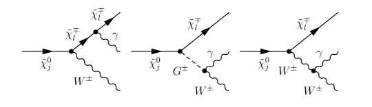
Figure 5: Real corrections for $\tilde{\chi}^{0}_{j}\rightarrow\tilde{\chi}^{\mp}_{l}W^{\pm}\gamma$.

Figure 6: Real corrections for $\tilde{\chi}^{\pm}_{l}\rightarrow\tilde{\chi}^{0}_{j}W^{\pm}\gamma$.

Denoting the width due to real bremsstrahlung by $\Gamma^{R}$ we obtain for the IR-finite decay width at next-to-leading order

$$\Gamma^{1}=\Gamma^{1L}+\Gamma^{R}\,.$$ (118)

5 Numerical results

Let us discuss a general feature before presenting our numerical results. Inspecting the couplings given in (24) one sees that only the wino and higgsino components of the neutralinos couple but not the bino or the singlino one. This implies a small tree-level width if the neutralino involved is either mainly bino or singlino which potentially results in large corrections to the widths considered as we will see below.

In the subsequent section we first present our results for the NMSSM benchmark points given in [35, 36]. Afterwards we consider cases where the neutralino is nearly a pure bino or singlino. There we demonstrate the additional corrections not considered so far as important as the squark/quark contributions considered in the literature [12].

5.1 NLO masses and decay widths for benchmark scenarios

In Table 1 we recall the most important parameters of the benchmark scenarios used in our analysis based on [35] and [36]. They are minimal supergravity (mSUGRA) [35] and gauge mediated SUSY breaking (GMSB) [36] scenarios. The parameter points can also be found within NMSSM-Tools [37].

		mSUGRA $1$	mSUGRA $3$	mSUGRA $4$
GUT	$M_{0}$ (in GeV)	$180$	$178$	$780$
scale	$M_{1/2}$ (in GeV)	$500$	$500$	$775$
	$A_{0}$ (in GeV)	$-1500$	$-1500$	$-2250$
SUSY	$\tan\beta(m_{Z})$	$10$	$10$	$2.6$
scale	$\mu$ (in GeV)	$969$	$938$	$-197$
	$\lambda,\kappa$	$0.10,0.10$	$0.40,0.30$	$0.52,0.10$
	$A_{\lambda},A_{\kappa}$ (in GeV)	$-959,-1.6$	$-616,-11$	$-557,20$
		GMSB $1$	GMSB $2$	GMSB $5$
Mess.	$M_{Mess}$ (in GeV)	$10^{13}$	$10^{13}$	$5\cdot 10^{14}$
scale	$\Lambda$ (in GeV)	$1.7\cdot 10^{5}$	$1.7\cdot 10^{5}$	$7.5\cdot 10^{4}$
SUSY	$\tan\beta(m_{Z})$	$8.5$	$1.63$	$50$
scale	$\mu$ (in GeV)	$1404$	$2351$	$1376$
	$\lambda,\kappa$	$0.020,0.004$	$0.50,0.43$	$0.010,-0.0007$
	$A_{\lambda},A_{\kappa}$ (in GeV)	$-52,-160$	$-446,-2300$	$118,4645$

Table 1: Most important parameters in the mSUGRA [35] and GMSB [36] benchmark scenarios.

Note, that we calculate the soft breaking masses $m_{H_{d}}^{2},m_{H_{u}}^{2}$ and in case of the NMSSM in addition $m_{S}^{2}$ from the tadpole equations, implying that they are not input parameters in CNNDecays . We do not give here the detailed soft SUSY breaking parameters but refer for this to [35] and [36] and/or the output of CNNDecays discussed in the appendix.

		mSUGRA $1$	mSUGRA $3$	mSUGRA $4$	GMSB $1$	GMSB $2$	GMSB $5$
$\tilde{\chi}^{0}_{1}:$	$m$	$210.79$	$210.97$	$89.08$	$472.48$	$472.53$	$203.30$
	$m^{1L}$	$210.61$	$210.77$	$91.45$	$472.38$	$472.39$	$203.30$
	$C$	$\tilde{B}$	$\tilde{B}$	$\tilde{S}$	$\tilde{B}$	$\tilde{B}$	$\tilde{S}$
$\tilde{\chi}^{0}_{2}:$	$m$	$387.18$	$387.47$	$215.38$	$620.06$	$855.54$	$496.87$
	$m^{1L}$	$387.10$	$387.37$	$215.58$	$620.06$	$855.53$	$496.81$
	$C$	$\tilde{W}$	$\tilde{W}$	$\tilde{H}$	$\tilde{S}$	$\tilde{W}$	$\tilde{B}$
$\tilde{\chi}^{0}_{3}:$	$m$	$971.11$	$942.27$	$217.09$	$854.13$	$2352.36$	$899.60$
	$m^{1L}$	$971.75$	$941.05$	$217.51$	$854.43$	$2352.49$	$899.98$
	$C$	$\tilde{H}$	$\tilde{H}$	$\tilde{H}$	$\tilde{W}$	$\tilde{H}$	$\tilde{W}$
$\tilde{\chi}^{0}_{4}:$	$m$	$976.52$	$943.16$	$330.51$	$1405.44$	$2355.92$	$1377.67$
	$m^{1L}$	$975.14$	$942.79$	$331.01$	$1405.15$	$2354.84$	$1377.45$
	$C$	$\tilde{H}$	$\tilde{H}$	$\tilde{B}$	$\tilde{H}$	$\tilde{H}$	$\tilde{H}$
$\tilde{\chi}^{0}_{5}:$	$m$	$2101.57$	$1421.70$	$608.43$	$1412.41$	$4062.82$	$1383.97$
	$m^{1L}$	$2101.57$	$1421.67$	$607.64$	$1411.46$	$4062.84$	$1383.04$
	$C$	$\tilde{S}$	$\tilde{S}$	$\tilde{W}$	$\tilde{H}$	$\tilde{S}$	$\tilde{H}$
$\tilde{\chi}^{\pm}_{1}:$	$m$	$387.16$	$387.48$	$201.36$	$854.11$	$855.53$	$899.59$
	$m^{1L}$	$387.23$	$387.53$	$201.73$	$854.57$	$855.69$	$900.14$
	$C$	$\tilde{W}^{\pm}$	$\tilde{W}^{\pm}$	$\tilde{H}^{\pm}$	$\tilde{W}^{\pm}$	$\tilde{W}^{\pm}$	$\tilde{W}^{\pm}$
$\tilde{\chi}^{\pm}_{2}:$	$m$	$977.07$	$947.45$	$608.40$	$1412.29$	$2355.33$	$1384.24$
	$m^{1L}$	$976.69$	$947.07$	$607.80$	$1411.62$	$2355.06$	$1383.51$
	$C$	$\tilde{H}^{\pm}$	$\tilde{H}^{\pm}$	$\tilde{W}^{\pm}$	$\tilde{H}^{\pm}$	$\tilde{H}^{\pm}$	$\tilde{H}^{\pm}$

Table 2: Neutralino and chargino masses $m$ on tree-level and $m^{1L}$ on one-loop-level in GeV and main particle character $C$ for the mSUGRA [35] and GMSB [36] benchmark scenarios.

Sc.	Decay	$\Gamma^{0}$ (in GeV)	$\Gamma^{1}$ (in GeV)	$\delta_{1(\tilde{q},q)}$	$\delta_{2}$	$\delta_{1+2}$
$1$	$\tilde{\chi}^{0}_{3}\rightarrow\tilde{\chi}^{-}_{1}W^{+}$	$2.153$	$2.234$	$1.8\%$	$2.0\%$	$3.8\%$
	$\tilde{\chi}^{0}_{4}\rightarrow\tilde{\chi}^{-}_{1}W^{+}$	$2.181$	$2.256$	$1.8\%$	$1.6\%$	$3.4\%$
	$\tilde{\chi}^{0}_{5}\rightarrow\tilde{\chi}^{-}_{1}W^{+}$	$3.206\cdot 10^{-3}$	$2.897\cdot 10^{-3}$	$-2.6\%$	$-7.0\%$	$-9.6\%$
	$\tilde{\chi}^{0}_{5}\rightarrow\tilde{\chi}^{-}_{2}W^{+}$	$1.542\cdot 10^{-1}$	$1.521\cdot 10^{-1}$	$-1.9\%$	$0.5\%$	$-1.4\%$
	$\tilde{\chi}^{-}_{1}\rightarrow\tilde{\chi}^{0}_{1}W^{-}$	$2.575\cdot 10^{-3}$	$2.561\cdot 10^{-3}$	$0.8\%$	$-1.3\%$	$-0.5\%$
	$\tilde{\chi}^{-}_{2}\rightarrow\tilde{\chi}^{0}_{1}W^{-}$	$5.860\cdot 10^{-1}$	$5.766\cdot 10^{-1}$	$0.2\%$	$-1.8\%$	$-1.6\%$
	$\tilde{\chi}^{-}_{2}\rightarrow\tilde{\chi}^{0}_{2}W^{-}$	$2.201$	$2.222$	$-0.3\%$	$1.2\%$	$0.9\%$
$3$	$\tilde{\chi}^{0}_{3}\rightarrow\tilde{\chi}^{-}_{1}W^{+}$	$2.085$	$2.153$	$1.8\%$	$1.5\%$	$3.3\%$
	$\tilde{\chi}^{0}_{4}\rightarrow\tilde{\chi}^{-}_{1}W^{+}$	$2.121$	$2.181$	$1.8\%$	$1.0\%$	$2.8\%$
	$\tilde{\chi}^{0}_{5}\rightarrow\tilde{\chi}^{-}_{1}W^{+}$	$2.937\cdot 10^{-2}$	$2.755\cdot 10^{-2}$	$-1.7\%$	$-4.5\%$	$-6.2\%$
	$\tilde{\chi}^{0}_{5}\rightarrow\tilde{\chi}^{-}_{2}W^{+}$	$1.302$	$1.352$	$-0.6\%$	$4.5\%$	$3.9\%$
	$\tilde{\chi}^{-}_{1}\rightarrow\tilde{\chi}^{0}_{1}W^{-}$	$2.951\cdot 10^{-3}$	$2.910\cdot 10^{-1}$	$0.7\%$	$-2.1\%$	$-1.4\%$
	$\tilde{\chi}^{-}_{2}\rightarrow\tilde{\chi}^{0}_{1}W^{-}$	$5.684\cdot 10^{-1}$	$5.552\cdot 10^{-1}$	$0.2\%$	$-2.5\%$	$-2.3\%$
	$\tilde{\chi}^{-}_{2}\rightarrow\tilde{\chi}^{0}_{2}W^{-}$	$2.115$	$2.141$	$0.6\%$	$0.6\%$	$1.2\%$
$4$	$\tilde{\chi}^{0}_{4}\rightarrow\tilde{\chi}^{-}_{1}W^{+}$	$4.719\cdot 10^{-2}$	$5.080\cdot 10^{-2}$	$-0.3\%$	$7.9\%$	$7.6\%$
	$\tilde{\chi}^{0}_{5}\rightarrow\tilde{\chi}^{-}_{1}W^{+}$	$7.442\cdot 10^{-1}$	$7.288\cdot 10^{-1}$	$0.2\%$	$-2.3\%$	$-2.1\%$
	$\tilde{\chi}^{-}_{1}\rightarrow\tilde{\chi}^{0}_{1}W^{-}$	$1.623\cdot 10^{-1}$	$1.650\cdot 10^{-1}$	$-0.9\%$	$2.5\%$	$1.6\%$
	$\tilde{\chi}^{-}_{2}\rightarrow\tilde{\chi}^{0}_{1}W^{-}$	$2.357\cdot 10^{-1}$	$2.291\cdot 10^{-1}$	$0.2\%$	$-3.0\%$	$-2.8\%$
	$\tilde{\chi}^{-}_{2}\rightarrow\tilde{\chi}^{0}_{2}W^{-}$	$5.758\cdot 10^{-1}$	$5.586\cdot 10^{-1}$	$0.2\%$	$-3.2\%$	$-3.0\%$
	$\tilde{\chi}^{-}_{2}\rightarrow\tilde{\chi}^{0}_{3}W^{-}$	$6.024\cdot 10^{-1}$	$5.875\cdot 10^{-1}$	$0.2\%$	$-2.7\%$	$-2.5\%$
	$\tilde{\chi}^{-}_{2}\rightarrow\tilde{\chi}^{0}_{4}W^{-}$	$7.007\cdot 10^{-2}$	$6.963\cdot 10^{-2}$	$-0.3\%$	$-0.3\%$	$-0.6\%$

Table 3: NLO corrections for the mSUGRA benchmark scenarios; $\delta$ is defined in (119).

Sc.	Decay	$\Gamma^{0}$ (in GeV)	$\Gamma^{1}$ (in GeV)	$\delta_{1(\tilde{q},q)}$	$\delta_{2}$	$\delta_{1+2}$
$1$	$\tilde{\chi}^{0}_{4}\rightarrow\tilde{\chi}^{-}_{1}W^{+}$	$2.891$	$3.068$	$-0.2\%$	$6.3\%$	$6.1\%$
	$\tilde{\chi}^{0}_{5}\rightarrow\tilde{\chi}^{-}_{1}W^{+}$	$2.943$	$3.114$	$-0.1\%$	$5.9\%$	$5.8\%$
	$\tilde{\chi}^{-}_{1}\rightarrow\tilde{\chi}^{0}_{1}W^{-}$	$1.027\cdot 10^{-2}$	$1.028\cdot 10^{-1}$	$0.0\%$	$0.1\%$	$0.1\%$
	$\tilde{\chi}^{-}_{1}\rightarrow\tilde{\chi}^{0}_{2}W^{-}$	$8.907\cdot 10^{-5}$	$8.942\cdot 10^{-5}$	$-0.1\%$	$0.5\%$	$0.4\%$
	$\tilde{\chi}^{-}_{2}\rightarrow\tilde{\chi}^{0}_{1}W^{-}$	$8.941\cdot 10^{-1}$	$8.795\cdot 10^{-1}$	$0.2\%$	$-1.8\%$	$-1.6\%$
	$\tilde{\chi}^{-}_{2}\rightarrow\tilde{\chi}^{0}_{2}W^{-}$	$3.787\cdot 10^{-3}$	$3.697\cdot 10^{-3}$	$-0.5\%$	$-1.9\%$	$-2.4\%$
	$\tilde{\chi}^{-}_{2}\rightarrow\tilde{\chi}^{0}_{3}W^{-}$	$2.962$	$3.126$	$-0.1\%$	$5.6\%$	$5.5\%$
$2$	$\tilde{\chi}^{0}_{3}\rightarrow\tilde{\chi}^{-}_{1}W^{+}$	$7.431$	$7.241$	$0.2\%$	$-2.8\%$	$-2.6\%$
	$\tilde{\chi}^{0}_{4}\rightarrow\tilde{\chi}^{-}_{1}W^{+}$	$7.442$	$7.254$	$0.4\%$	$-2.9\%$	$-2.5\%$
	$\tilde{\chi}^{0}_{5}\rightarrow\tilde{\chi}^{-}_{1}W^{+}$	$1.164\cdot 10^{-2}$	$9.868\cdot 10^{-3}$	$-3.4\%$	$-11.8\%$	$-15.2\%$
	$\tilde{\chi}^{0}_{5}\rightarrow\tilde{\chi}^{-}_{2}W^{+}$	$1.890$	$1.851$	$-2.0\%$	$-0.1\%$	$-2.1\%$
	$\tilde{\chi}^{-}_{1}\rightarrow\tilde{\chi}^{0}_{1}W^{-}$	$6.150\cdot 10^{-3}$	$6.135\cdot 10^{-3}$	$0.0\%$	$-0.2\%$	$-0.2\%$
	$\tilde{\chi}^{-}_{2}\rightarrow\tilde{\chi}^{0}_{1}W^{-}$	$1.807$	$1.708$	$-0.7\%$	$-4.8\%$	$-5.5\%$
	$\tilde{\chi}^{-}_{2}\rightarrow\tilde{\chi}^{0}_{2}W^{-}$	$7.491$	$7.235$	$0.3\%$	$-3.7\%$	$-3.4\%$
$5$	$\tilde{\chi}^{0}_{4}\rightarrow\tilde{\chi}^{-}_{1}W^{+}$	$2.283$	$2.439$	$-0.3\%$	$7.1\%$	$6.8\%$
	$\tilde{\chi}^{0}_{5}\rightarrow\tilde{\chi}^{-}_{1}W^{+}$	$2.333$	$2.485$	$-0.1\%$	$6.6\%$	$6.5\%$
	$\tilde{\chi}^{-}_{1}\rightarrow\tilde{\chi}^{0}_{1}W^{-}$	$1.462\cdot 10^{-5}$	$1.453\cdot 10^{-5}$	$-0.3\%$	$-0.3\%$	$-0.6\%$
	$\tilde{\chi}^{-}_{1}\rightarrow\tilde{\chi}^{0}_{2}W^{-}$	$8.424\cdot 10^{-3}$	$8.407\cdot 10^{-3}$	$-0.1\%$	$-0.1\%$	$-0.2\%$
	$\tilde{\chi}^{-}_{2}\rightarrow\tilde{\chi}^{0}_{1}W^{-}$	$1.279\cdot 10^{-3}$	$1.242\cdot 10^{-3}$	$-0.6\%$	$-2.2\%$	$-2.9\%$
	$\tilde{\chi}^{-}_{2}\rightarrow\tilde{\chi}^{0}_{2}W^{-}$	$7.898\cdot 10^{-1}$	$7.775\cdot 10^{-1}$	$-0.1\%$	$-1.5\%$	$-1.6\%$
	$\tilde{\chi}^{-}_{2}\rightarrow\tilde{\chi}^{0}_{3}W^{-}$	$2.339$	$2.486$	$-0.1\%$	$6.4\%$	$6.3\%$

Table 4: NLO corrections for the GMSB benchmark scenarios; $\delta$ is defined in (119).

We show the corresponding masses $m$, one-loop masses $m^{1L}$ and particle characters $C$ in Table 2. In Tables 3 and 4 we present our results for the decay widths in the mSUGRA and GMSB scenarios, respectively. Tables 3 and 4 contain beside the tree-level and one-loop corrected widths the correction factor

$$\delta=\frac{\Gamma^{1}-\Gamma^{0}}{\Gamma^{0}}\qquad,$$ (119)

which is also split in the parts $\delta_{1}=\delta_{1(\tilde{q},q)}$ due to squark and quark corrections and $\delta_{2}$ containing the other contributions, which includes the hard photon emission for comparison with [12]. As already stated, the mass corrections $m\rightarrow m^{1L}$ presented in Table 2 are small, in most cases in the per-mil range. Only the light Singlino in the mSUGRA $4$ scenario gets a large correction of $2.6$% from squark and quark contributions.

As expected the widths are larger in case the neutralino involved has either large wino and/or higgsino components. Note, that from (24) follows that the $W$ boson couples either to a wino-wino or a higgsino-higgsino combination. This explains several of at first glance surprising features, e.g. the fact that in mSUGRA scenarios $1$ and $3$ the width $\Gamma(\tilde{\chi}^{0}_{5}\rightarrow\tilde{\chi}^{+}_{2}W^{-})$ is larger than $\Gamma(\tilde{\chi}^{0}_{5}\rightarrow W^{-}\tilde{\chi}^{+}_{1})$ despite the smaller phase space. Another surprise might be the difference in $\delta_{2}$ for the decay $\tilde{\chi}_{2}^{-}\rightarrow\tilde{\chi}_{1}^{0}W^{-}$ in scenarios mSUGRA $1$ and mSUGRA $3$. However this can be understood from the differences in the Higgs sector. We see that the corrections are in general in the order of $1$-$3\%$ but can easily go up to $10\%$. Note, that depending on the parameters the corrections can have both signs.

5.2 NLO corrections in case of bino and singlino like neutralinos

It follows from (24) that the partial width into a $W$-boson vanishes in the limit that the neutralino involved is either a pure bino or a pure singlino. This is the main reason that in Tables 3 and 4 the processes containing states which are to a large extent bino or singlino have small widths. However, even in the limit of pure states the corresponding couplings are induced at the one-loop level. In this section we investigate this in more detail. We consider here a wide mass range and are aware that neutralinos with masses above 1 TeV will hardly be produced at LHC and will therefore most likely require a multi-TeV lepton collider such as CLIC. All the plots and decay widths are based on tree-level masses $m_{\tilde{\chi}_{i}^{\pm 0}}$ for neutralinos and charginos. The corresponding plots with the one-loop corrected masses differ only slightly and the differences are hardly visible.

5.2.1 Bino decays

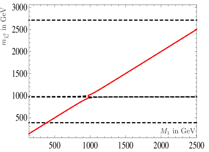
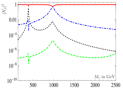
Figure 7: a) (left): Neutralino masses as a function of $M_{1}$ and the other parameters according to mSUGRA $1$ apart from $\kappa=0.14$. The red solid line marks $\tilde{B}$ whereas the other states are shown with black dashed lines. b) (right): Particle character for the bino state $\tilde{B}$ as a function of $M_{1}$: red (solid): Bino character $|\mathcal{N}_{j1}|^{2}$, blue (dot-dashed): Higgsino character $|\mathcal{N}_{j3}|^{2}+|\mathcal{N}_{j4}|^{2}$, black (dotted): Wino character $|\mathcal{N}_{j2}|^{2}$, green (dashed): Singlino character $|\mathcal{N}_{j5}|^{2}$.

We define a state denoted by $\tilde{B}$ to be bino-like if $|\mathcal{N}_{j1}|^{2}>0.5$. We take benchmark point mSUGRA $1$ and vary the gaugino mass $M_{1}$ for our subsequent numerical investigations. Moreover, we shift $\kappa$ from $0.11$ to $0.14$ to disentangle different effects and to simplify the discussion. The corresponding neutralino mass spectrum is shown in Figure 7 a) as a function of $M_{1}$ and the particle character of the corresponding mainly bino-like state $\tilde{B}$ is shown in Figure 7 b). Note that at the various crossings in plot a) the index of the corresponding neutralino mass eigenstate changes.

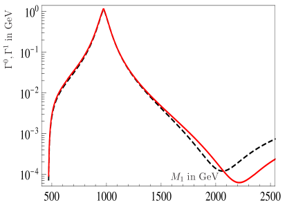
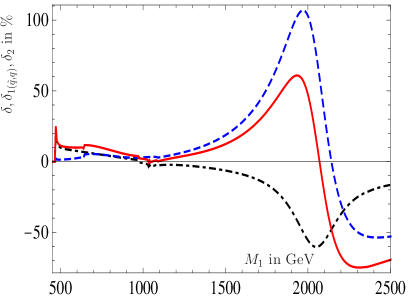
Figure 8: a) (left): LO (black, dashed) and NLO (red, solid) decay widths for $\tilde{B}\rightarrow\tilde{\chi}_{1}^{-}W^{+}$ as a function of $M_{1}$ for the spectrum of Figure 7, b) (right): Correction factor $\delta$ in % defined in (119) for $\tilde{B}\rightarrow\tilde{\chi}_{1}^{-}W^{+}$ as a function of $M_{1}$: blue (dashed): Squark and quark contributions, black (dot-dashed): Other sectors, red (solid): Full correction.

Figure 8 a) shows the LO and NLO decay width of $\tilde{B}\rightarrow\tilde{\chi}_{1}^{-}W^{+}$ as a function of $M_{1}$. At $M_{1}\simeq 1$ TeV the level crossing with the higgsino like states occurs giving rise to the observed rise of the width with $M_{1}$ and the subsequent decrease. In the later case the decrease is strengthened by a negative interference of the higgsino and wino parts. Moreover we note that here and also in the corresponding figures below a Coloumb singularity occurs close to the kinematical threshold, e.g. close to $m_{\tilde{B}}=m_{\tilde{\chi}^{\pm}_{1}}+m_{W}$, which has to be resumed. As this has not been done, we start our plots slightly above this region.

The relative size of the corrections are shown in Figure 8 b) where we also compare the third generation squark/quark contribution with the additional ones. The kinks correspond to the level crossings in Figure 7. Note that both parts of the correction can be of equal importance and that in some regions of the parameter space they cancel partly each other whereas there are also regions where they point in the same direction. It is remarkable that the loop induced corrections can be of the same order of magnitude as the tree-level widths. This however does not imply a break-down of perturbation theory but is a consequence that in the limit of a pure bino the tree-level coupling vanishes but the one-loop induced one is non-zero.

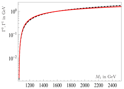
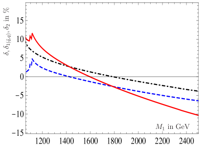
Figure 9: a) (left): LO (black, dashed) and NLO (red, solid) decay widths for $\tilde{B}\rightarrow\tilde{\chi}_{2}^{-}W^{+}$ as a function of $M_{1}$ for the spectrum of Figure 7, b) (right): Correction factor $\delta$ in % defined in (119) for $\tilde{B}\rightarrow\tilde{\chi}_{2}^{-}W^{+}$ as a function of $M_{1}$: blue (dashed): Squark and quark contributions, black (dot-dashed): Other sectors, red (solid): Full correction.

Figure 9 a) shows the widths for the decay $\tilde{B}\rightarrow\tilde{\chi}_{2}^{-}W^{+}$ as a function of $M_{1}$. In contrast to the decay into $\tilde{\chi}_{1}^{-}$ there is a positive interference of the wino-wino and higgsino-higgsino components in the LO couplings (24). Note, that the decrease of the couplings for increasing $M_{1}$ is compensated by a factor $(M_{1}/m_{W})^{2}$, see Equations (3.2)–(29) leading to a slight increase of the width with increasing $M_{1}$. Also in this case the corrections can be sizable amounting up to about $15$ percent.

5.2.2 Singlino decays

The case of a singlino-like neutralino $\tilde{S}$, defined by $|N_{j5}|^{2}>0.5$, shows similar features to the case of a bino-like neutralino. However, there is one important difference: In the limit of a pure singlino it only couples to the doublet Higgs/higgsino states and the singlet Higgs boson. Hence one expects that the squark/quark contributions to be of less importance compared to the bino case.

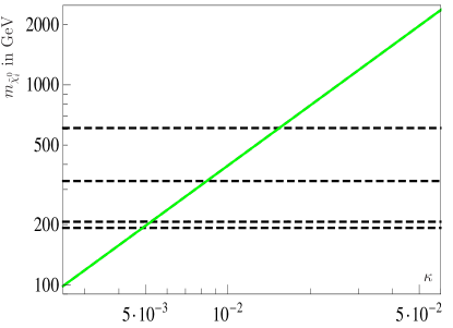
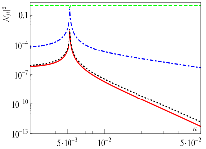
Figure 10: a) (left): Neutralino masses as a function of $\kappa$ and the other parameters according to mSUGRA $4$ apart from $\lambda=0.01$. The green solid line marks $\tilde{S}$ whereas the other states are shown with black dashed lines. b) (right): Particle character for the singlino state $\tilde{S}$ as a function of $\kappa$: red (solid): Bino character $|\mathcal{N}_{j1}|^{2}$, blue (dot-dashed): Higgsino character $|\mathcal{N}_{j3}|^{2}+|\mathcal{N}_{j4}|^{2}$, black (dotted): Wino character $|\mathcal{N}_{j2}|^{2}$, green (dashed): Singlino character $|\mathcal{N}_{j5}|^{2}$.

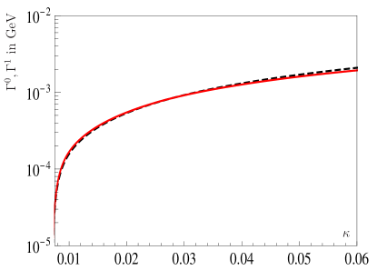
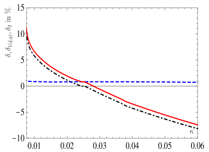
Figure 11: a) (left): LO (black, dashed) and NLO (red, solid) decay widths for $\tilde{S}\rightarrow\tilde{\chi}_{1}^{-}W^{+}$ as a function of $\kappa$ for the spectrum of Figure 10, b) (right): Correction factor $\delta$ in % defined in (119) for $\tilde{S}\rightarrow\tilde{\chi}_{1}^{-}W^{+}$ as a function of $\kappa$: blue (dashed): Squark and quark contributions, black (dot-dashed): Other sectors, red (solid): Full correction.

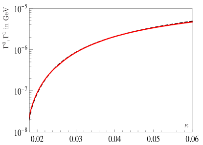
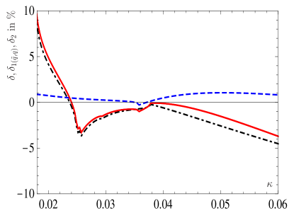
Figure 12: a) (left) LO (black, dashed) and NLO (red, solid) decay widths for $\tilde{S}\rightarrow\tilde{\chi}_{2}^{-}W^{+}$ as a function of $\kappa$ for the spectrum of Figure 10, b) (right): Correction factor $\delta$ in % defined in (119) for $\tilde{S}\rightarrow\tilde{\chi}_{2}^{-}W^{+}$ as a function of $\kappa$: blue (dashed): Squark and quark contributions, black (dot-dashed): Other sectors, red (solid): Full correction.

For the numerical investigation we choose the benchmark scenario mSUGRA $4$, but reduce $\lambda$ to $\lambda=0.01$ to increase the singlino character. We vary $\kappa$ between $2\cdot 10^{-3}$ and $6\cdot 10^{-2}$ leading to singlino masses between $100$ GeV and $2.5$ TeV. In this rather light particle spectrum the higgsino-like chargino has a mass of $m_{\tilde{\chi}_{1}^{\pm}}=201$ GeV and the wino-like chargino has a mass of $m_{\tilde{\chi}_{2}^{\pm}}=608$ GeV. The mass spectrum of the neutralinos is given in Figure 10 a).

In Figure 11 we show the details for the decay $\tilde{S}\rightarrow\tilde{\chi}_{1}^{-}W^{+}$. Note that despite the decrease of the coupling due to the decrease in the wino and higgsino components with increasing $\kappa$ one gets a net increase of the width due to the $(m_{\tilde{S}}/m_{W})^{2}$ factor. In the right plot one sees clearly that contributions of third generation squarks and quarks are less important compared to the bino case. However, the remaining contribution can amount up to about 10 percent. Also the decay into the heavier chargino shows similar features as can be seen from Figure 12. The main difference is that the threshold effects due to on-shell intermediate states are more pronounced in this case and are mainly caused by sleptons and Higgs bosons at $m_{\tilde{S}}\approx 1$ TeV and by squarks at $m_{\tilde{S}}\approx 1.6$ TeV.

5.2.3 Chargino decays

In this section we present the decays of the wino-like chargino $\tilde{W}^{+}$ in a bino- or singlino-like neutralino $\tilde{\chi}_{1,2}^{0}$, being the two lightest neutralinos in the benchmark scenario GMSB $5$. We depart from the original parameters by setting $M_{1}=300$ GeV and $\mu=600$ GeV to get a rather light particle spectrum. We vary the gaugino mass $M_{2}$ between $100$ and $2000$ GeV. The neutralino mass spectrum is given in Figure 13 a) and the chargino mass spectrum in Figure 13 b). The two light neutralinos have a mass of $m_{\tilde{\chi}_{1}^{0}}=89$ GeV for the singlino-like neutralino and $m_{\tilde{\chi}_{2}^{0}}=298$ GeV for the bino-like neutralino.

In Figures 14 and 15 we show the details of the decays $\tilde{W}^{+}\rightarrow\tilde{\chi}^{0}_{1,2}W^{+}$. Note that the peaks close to $M_{2}\approx 620$ GeV are due to the level crossing of the wino-like states with the higgsino-like states. The overall features of the widths and corrections are similar to the case of neutralino decays. In general the corrections are in the order of a few percent except for a region close to $M_{2}=1.15$ TeV for the decay $\tilde{W}^{+}\rightarrow\tilde{\chi}_{2}^{0}W^{+}$ in Figure 15 where the tree-level couplings to $\tilde{\chi}^{0}_{2}$ nearly vanish due to a negative interference between the wino and higgsino contributions. We find that the third generation squark/quark contributions are in general somewhat smaller than the remaining ones.

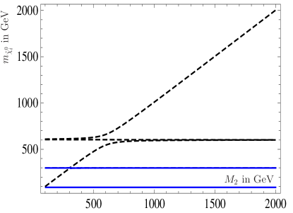
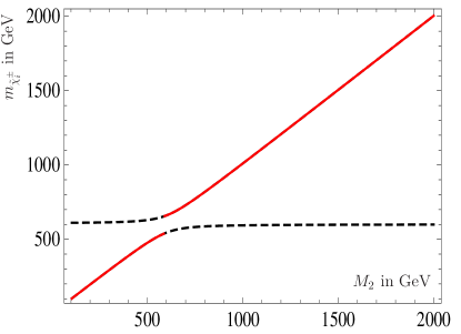
Figure 13: a) (left): Neutralino masses and b) (right): Chargino masses as a function of $M_{2}$. The other parameters are as GMSB $5$ apart from $M_{1}=300$ GeV and $\mu=600$ GeV. The red lines in b) correspond to the wino like states and the two blue ones in a) to the singlino state $\tilde{\chi}_{1}^{0}$ and bino state $\tilde{\chi}_{2}^{0}$.

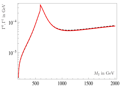
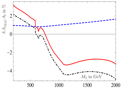
Figure 14: a) (left): LO (black, dashed) and NLO (red, solid) decay widths for $\tilde{W}^{+}\rightarrow\tilde{\chi}_{1}^{0}W^{+}$ as a function of $M_{2}$ for the spectrum of Figure 13, b) (right): Correction factor $\delta$ in % defined in (119) for $\tilde{W}^{+}\rightarrow\tilde{\chi}_{1}^{0}W^{+}$ as a function of $M_{2}$: blue (dashed): Squark and quark contributions, black (dot-dashed): Other sectors, red (solid): Full correction.

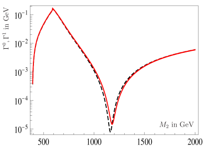
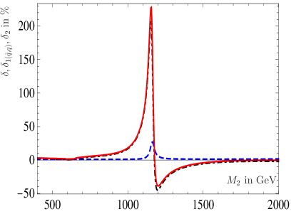
Figure 15: a) (left): LO (black, dashed) and NLO (red, solid) decay widths for $\tilde{W}^{+}\rightarrow\tilde{\chi}_{2}^{0}W^{+}$ as a function of $M_{2}$ for the spectrum of Figure 13, b) (right): Correction factor $\delta$ in % defined in (119) for $\tilde{W}^{+}\rightarrow\tilde{\chi}_{2}^{0}W^{+}$ as a function of $M_{2}$: blue (dashed): Squark and quark contributions, black (dot-dashed): Other sectors, red (solid): Full correction.

6 Conclusion

In this paper we presented the complete electroweak one-loop corrections to the partial widths for two-body decays of a chargino (neutralino) into a $W$-boson and a neutralino (chargino). The calculations were done for the MSSM and the NMSSM using an on-shell scheme and we have used the so-called pinch technique to achieve gauge invariance. Moreover we based the calculation of one-loop masses for neutralinos and charginos on a reasonable renormalization of the physical parameters, which are present on tree-level.

Whereas the mass corrections to neutralinos and charginos are typically in the per-mil range, the corrections to the decays are in the order of $1$-$10$ percent, in particular if the involved neutralino is either wino or higgsino like. However in case of a small leading order decay width the corrections can be $50$ percent or larger. This is the case if either there is a negative interference between the wino and the higgsino part of the couplings or if the neutralino is either mainly bino- or singlino-like, because for a pure bino or a pure singlino the tree-level width is identical zero and can only be induced at the 1-loop level. Last but not least we provide the publicly available program CNNDecays for the numerical evaluation.

7 Acknowledgments

This work has been supported by the DFG, Project no. PO-1337/2-1. S.L. has been supported by the DFG research training group GRK1147. We thank Sven Heinemeyer, Federico von der Pahlen and Christian Schappacher for pointing out an error in the renormalization of the electric charge and for a detailed comparison of the Bremsstrahlung integrals.

Appendix A Formulas: Vertex corrections

In this section we present the generic formulas for the next-to leading order vertex contributions for the ’t Hooft-Feynman gauge $\xi_{V}=1$ ($V=W,Z$). The formulas for $\xi_{V}\neq 1$ are contained in the program CNNDecays [34]. The formulas for the self-energies can be found in [38], from which also the derivatives with respect to $p^{2}$ can be calculated. They are also included in CNNDecays [34].

Below we present the formulas for the generic contributions to the matrix element $M_{V}$ shown in Figure 4. In addition we give the particle combinations to be inserted in these diagrams for the decay $\tilde{\chi}^{0}\rightarrow\tilde{\chi}^{-}W^{+}$ neglecting generation indices. We use the following notation: $H$ stands for one of the $2(3)$ scalar Higgs bosons, $A$ for one of the $2(3)$ pseudoscalar Higgs bosons including the Goldstone boson and $H^{\pm}$ for one of the $2$ charged scalars including the Goldstone boson. The indices of couplings and masses in the generic formulas have to be understood in the following form: $F_{i}$ and $F_{o}$ denote the decaying and outgoing fermion, $W$ the external $W$-boson, whereas $F$, $F_{1,2}$, $S$, $S_{1,2}$, $V$ or $V_{1,2}$ represent possible internal fermionic, scalar or vector particles. It is understood implicitly that one has to sum over possible flavour and generation indices of the internal particles. All contributions have the same generic structure:

$$M_{V}= \frac{i}{16\pi^{2}}\overline{u}(p_{1})\gamma^{\mu}\left(P_{L}M_{1}+P_{R}M_{2}\right)u(k)\epsilon_{\mu}^{*}(p_{2})$$ (120)

$$+ \frac{i}{16\pi^{2}}\overline{u}(p_{1})\left(P_{L}M_{3}^{\mu}+P_{R}M_{4}^{\mu}\right)u(k)\epsilon_{\mu}^{*}(p_{2})$$

We start with the vertex in Figure 4 a) containing two internal fermions and one scalar. We use the following abbreviations for the couplings:

$$O_{1} =O_{FFV,L}(F_{2},F_{1},W),\qquad O_{2}=O_{FFV,R}(F_{2},F_{1},W)$$ (121)

$$O_{3} =O_{FFS,L}(F_{1},F_{i},S),\qquad O_{4}=O_{FFS,R}(F_{1},F_{i},S)$$ (122)

$$O_{5} =O_{FFS,L}(F_{o},F_{2},S),\qquad O_{6}=O_{FFS,R}(F_{o},F_{2},S)$$ (123)

In the formulas below the Passarino-Veltman integrals have as arguments: $B_{0}(m_{W}^{2},m_{F_{2}}^{2},m_{F_{1}}^{2})$ and $C_{i},C_{ij}(m_{W}^{2},m_{i}^{2},m_{o}^{2},m_{F_{2}}^{2},m_{F_{1}}^{2},m_{S}^{2})$. Possible particle insertions in the notation $SF_{1}F_{2}$ are given by $H\tilde{\chi}^{0}\tilde{\chi}^{\pm}$, $A\tilde{\chi}^{0}\tilde{\chi}^{\pm}$, $H^{\pm}\tilde{\chi}^{\pm}\tilde{\chi}^{0}$, $\tilde{\nu}\nu l$, $\tilde{l}l\nu$, $\tilde{u}ud$, $\tilde{d}du$. We get:

$$M_{1,a}= -O_{1}\left[O_{3}m_{F_{1}}(O_{6}m_{F_{2}}C_{0}-O_{5}m_{o}C_{1})+O_{4}O_{6}m_{F_{2}}m_{i}(C_{0}+C_{1})\right]$$ (124)

$$+O_{1}O_{5}m_{o}C_{2}(O_{3}m_{F_{1}}+O_{4}m_{i})+O_{2}\left[O_{3}(O_{6}(m_{S}^{2}C_{0}+m_{i}^{2}C_{1}+B_{0}-2C_{00}\right.$$

$$\left.-m_{o}^{2}(C_{0}+C_{1}+C_{2}))-O_{5}m_{F_{2}}m_{o}(C_{0}+C_{1}+C_{2}))+O_{4}O_{6}m_{F_{1}}m_{i}C_{1}\right]$$

$$M_{2,a}= O_{1}\left\{O_{3}O_{5}m_{F_{1}}m_{i}C_{1}+O_{4}\left[O_{5}(m_{S}^{2}C_{0}+m_{i}^{2}C_{1}-m_{o}^{2}(C_{0}+C_{1}+C_{2})\right.\right.$$ (125)

$$\left.\left.+B_{0}-2C_{00})-O_{6}m_{F_{2}}m_{o}(C_{0}+C_{1}+C_{2})\right]\right\}$$

$$+O_{2}\left\{O_{3}m_{i}(O_{6}m_{o}C_{2}-O_{5}m_{F_{2}}(C_{0}+C_{1}))\right.$$

$$\left.+O_{4}m_{F_{1}}(O_{6}m_{o}(C_{1}+C_{2})-O_{5}m_{F_{2}}C_{0})\right\}$$

$$M_{3,a}^{\mu}= p_{1}^{\mu}2\left\{O_{1}O_{4}\left[O_{5}m_{o}(C_{12}+C_{2}+C_{22})-O_{6}m_{F_{2}}(C_{0}+C_{1}+C_{2})\right]\right.$$ (126)

$$\left.+O_{2}O_{6}(O_{4}m_{F_{1}}C_{1}-O_{3}m_{i}C_{12})\right\}$$

$$+p_{2}^{\mu}2\left\{O_{2}O_{6}\left[O_{3}m_{i}(C_{1}+C_{12})+O_{4}m_{F_{1}}C_{1}\right]-O_{1}O_{4}O_{5}m_{o}(C_{1}+2C_{12})\right\}$$

$$M_{4,a}^{\mu}= p_{1}^{\mu}2\left\{O_{1}O_{5}(O_{3}m_{F_{1}}C_{1}-O_{4}m_{i}C_{12})\right.$$ (127)

$$\left.+O_{2}O_{3}\left[O_{6}m_{o}(C_{12}+C_{2}+C_{22})-O_{5}m_{F_{2}}(C_{0}+C_{1}+C_{2})\right]\right\}$$

$$+p_{2}^{\mu}2\left\{O_{1}O_{5}(O_{3}m_{F_{1}}C_{1}+O_{4}m_{i}(C_{1}+C_{12}))-O_{2}O_{3}O_{6}m_{o}(C_{1}+2C_{12})\right\}$$

For the vertex in Figure 4 b) we define:

$$O_{1} =O_{SSV}(S_{1},S_{2},V)$$ (128)

$$O_{2} =O_{FFS,L}(F,F_{i},S_{1}),\qquad O_{3}=O_{FFS,R}(F,F_{i},S_{1})$$ (129)

$$O_{4} =O_{FFS,L}(F_{o},F,S_{2}),\qquad O_{5}=O_{FFS,R}(F_{o},F,S_{2})$$ (130)

For completeness we note that in case of $O_{1}$ the following internal momentum combination appears $(p_{S_{1}}-p_{S_{2}})$ over which of course has been integrated. The Passarino-Veltman integrals below have the arguments $C_{i},C_{ij}(m_{o}^{2},m_{W}^{2},m_{i}^{2},m_{F}^{2},m_{S_{2}}^{2},m_{S_{1}}^{2})$. Possible particle insertions in the notation $FS_{1}S_{2}$ are given by $\tilde{\chi}^{0}HH^{\pm}$, $\tilde{\chi}^{\pm}H^{\pm}H$, $\tilde{\chi}^{0}AH^{\pm}$, $\tilde{\chi}^{\pm}H^{\pm}A$, $\nu\tilde{\nu}\tilde{l}$, $l\tilde{l}\tilde{\nu}$, $u\tilde{u}\tilde{d}$, $d\tilde{d}\tilde{u}$. We obtain for the different parts:

$$M_{1,b}= 2O_{1}O_{2}O_{5}C_{00}$$ (131)

$$M_{2,b}= 2O_{1}O_{3}O_{4}C_{00}$$ (132)

$$M_{3,b}^{\mu}= p_{2}^{\mu}O_{1}\left\{O_{3}(O_{5}m_{F}(C_{0}+2C_{2})-O_{4}m_{o}(C_{1}+2C_{12}))\right.$$ (133)

$$\left.-O_{2}O_{5}m_{i}(C_{2}+2C_{22})\right\}-2p_{1}^{\mu}O_{1}\left\{O_{2}O_{5}m_{i}(C_{12}+C_{2}+C_{22})\right.$$

$$\left.+O_{3}\left[O_{4}m_{o}(C_{1}+C_{11}+C_{12})-O_{5}m_{F}(C_{0}+C_{1}+C_{2})\right]\right\}$$

$$M_{4,b}^{\mu}= 2p_{1}^{\mu}O_{1}\left\{O_{2}\left[O_{4}m_{F}(C_{0}+C_{1}+C_{2})-O_{5}m_{o}(C_{1}+C_{11}+C_{12})\right]\right.$$ (134)

$$\left.-O_{3}O_{4}m_{i}(C_{12}+C_{2}+C_{22})\right\}+p_{2}^{\mu}O_{1}\left\{O_{2}\left[O_{4}m_{F}(C_{0}+2C_{2})\right.\right.$$

$$\left.\left.-O_{5}m_{o}(C_{1}+2C_{12})\right]-O_{3}O_{4}m_{i}(C_{2}+2C_{22})\right\}$$

For the vertex in Figure 4 c) we define:

$$O_{1} =O_{FFV,L}(F_{1},F_{i},V),\qquad O_{2}=O_{FFV,R}(F_{1},F_{i},V)$$ (135)

$$O_{3} =O_{FFV,L}(F_{2},F_{1},W),\qquad O_{4}=O_{FFV,R}(F_{2},F_{1},W)$$ (136)

$$O_{5} =O_{FFV,L}(F_{o},F_{2},V),\qquad O_{6}=O_{FFV,R}(F_{o},F_{2},V)$$ (137)

The Passarino-Veltman integrals below have as arguments $C_{i},C_{ij}(m_{W}^{2},m_{i}^{2},m_{o}^{2},m_{F_{2}}^{2},m_{F_{1}}^{2},m_{V}^{2})$ and $B_{0}(m_{W}^{2},m_{F_{2}}^{2},m_{F_{1}}^{2})$. Possible particle insertions in the notation $VF_{1}F_{2}$ are given by $Z\tilde{\chi}^{0}\tilde{\chi}^{\pm}$, $W\tilde{\chi}^{\pm}\tilde{\chi}^{0}$. We get:

$$M_{1,c}= 2O_{1}O_{5}\left\{O_{3}\left[m_{V}^{2}C_{0}+m_{i}^{2}(C_{1}-C_{2})-m_{o}^{2}(C_{0}+C_{1}+2C_{2})\right.\right.$$ (138)

$$\left.\left.+m_{W}^{2}C_{2}+B_{0}-2C_{00}\right]-O_{4}m_{F_{1}}m_{F_{2}}C_{0}\right\}-2O_{2}O_{4}O_{6}m_{i}m_{o}C_{2}$$

$$M_{2,c}= 2O_{2}O_{6}\left\{O_{4}\left[m_{V}^{2}C_{0}+m_{i}^{2}(C_{1}-C_{2})-m_{o}^{2}(C_{0}+C_{1}+2C_{2})\right.\right.$$ (139)

$$\left.\left.+m_{W}^{2}C_{2}+B_{0}-2C_{00}\right]-O_{3}m_{F_{1}}m_{F_{2}}C_{0}\right\}-2O_{1}O_{3}O_{5}m_{i}m_{o}C_{2}$$

$$M_{3,c}^{\mu}= 4p_{1}^{\mu}\left\{O_{2}\left[O_{3}O_{5}m_{F_{1}}C_{2}+O_{4}(O_{5}m_{F_{2}}C_{2}+O_{6}m_{o}(C_{2}+C_{22}))\right]\right.$$ (140)

$$\left.-O_{1}O_{3}O_{5}m_{i}(C_{2}+C_{12})\right\}-4p_{2}^{\mu}\left\{O_{2}\left[O_{3}O_{5}m_{F_{1}}C_{1}+O_{4}(O_{5}m_{F_{2}}(C_{0}+C_{1})\right.\right.$$

$$\left.\left.+O_{6}m_{o}(C_{1}+C_{11}+C_{12}+C_{2}))\right]-O_{1}O_{3}O_{5}m_{i}(C_{1}+C_{11})\right\}$$

$$M_{4,c}^{\mu}= 4p_{1}^{\mu}\left\{O_{1}\left[O_{3}(O_{5}m_{o}(C_{12}+C_{22})+O_{6}m_{F_{2}}C_{2})+O_{4}O_{6}m_{F_{1}}C_{2}\right]\right.$$ (141)

$$\left.-O_{2}O_{4}O_{6}m_{i}(C_{2}+C_{12})\right\}-4p_{2}^{\mu}\left\{O_{1}\left[O_{3}(O_{5}m_{o}(C_{1}+C_{11}+C_{12}+C_{2})\right.\right.$$

$$\left.\left.+O_{6}m_{F_{2}}(C_{0}+C_{1}))+O_{4}O_{6}m_{F_{1}}C_{1}\right]-O_{2}O_{4}O_{6}m_{i}(C_{1}+C_{11})\right\}$$

For the vertex in Figure 4 d) we define:

$$O_{1} =O_{FFV,L}(F_{o},F,V),\qquad O_{2}=O_{FFV,R}(F_{o},F,V)$$ (142)

$$O_{3} =O_{FFS,L}(F,F_{i},S),\qquad O_{4}=O_{FFS,R}(F,F_{i},S)$$ (143)

$$O_{5} =O_{SVV}(S,W,V)$$ (144)

The Passarino-Veltman integrals below have as arguments $C_{i},C_{ij}(m_{o}^{2},m_{W}^{2},m_{i}^{2},m_{F}^{2},m_{V}^{2},m_{S}^{2})$. Possible particle insertions in the notation $FSV$ are given by $\tilde{\chi}^{\pm}H^{\pm}\gamma$, $\tilde{\chi}^{\pm}H^{\pm}Z$, $\tilde{\chi}^{0}HW$, $\tilde{\chi}^{0}AW$. We get:

$$M_{1,d}= O_{5}(O_{1}O_{3}m_{F}C_{0}-O_{1}O_{4}m_{i}C_{2}+O_{2}O_{3}m_{o}C_{1})$$ (145)

$$M_{2,d}= O_{5}(O_{1}O_{4}m_{o}C_{1}-O_{2}O_{3}m_{i}C_{2}+O_{2}O_{4}m_{F}C_{0})$$ (146)

$$M_{3,d}^{\mu}= 2p_{1}^{\mu}O_{1}O_{4}O_{5}C_{1}$$ (147)

$$M_{4,d}^{\mu}= 2p_{1}^{\mu}O_{2}O_{3}O_{5}C_{1}$$ (148)

For the vertex in Figure 4 e) we define:

$$O_{1} =O_{FFV,L}(F,F_{i},V),\qquad O_{2}=O_{FFV,R}(F,F_{i},V)$$ (149)

$$O_{3} =O_{FFS,L}(F_{o},F,S),\qquad O_{4}=O_{FFS,R}(F_{o},F,S)$$ (150)

$$O_{5} =O_{SVV}(S,W,V)$$ (151)

The Passarino-Veltman integrals, which appear in the following formulas, have as arguments $C_{i},C_{ij}(m_{i}^{2},m_{W}^{2},m_{o}^{2},m_{F}^{2},m_{V}^{2},m_{S}^{2})$. Possible particle insertions in the notation $FVS$ are given by $\tilde{\chi}^{0}ZH^{\pm}$, $\tilde{\chi}^{\pm}WH$, $\tilde{\chi}^{\pm}WA$. We obtain:

$$M_{1,e}= O_{5}(-O_{1}O_{3}m_{o}C_{2}+O_{1}O_{4}m_{F}C_{0}+O_{2}O_{4}m_{i}C_{1})$$ (152)

$$M_{2,e}= O_{5}(O_{1}O_{3}m_{i}C_{1}+O_{2}O_{3}m_{F}C_{0}-O_{2}O_{4}m_{o}C_{2})$$ (153)

$$M_{3,e}^{\mu}= 2(p_{1}^{\mu}+p_{2}^{\mu})O_{2}O_{4}O_{5}C_{1}$$ (154)

$$M_{4,e}^{\mu}= 2(p_{1}^{\mu}+p_{2}^{\mu})O_{1}O_{3}O_{5}C_{1}$$ (155)

For the vertex in Figure 4 f) we define:

$$O_{1} =O_{FFV,L}(F,F_{i},V_{1}),O_{2}=O_{FFV,R}(F,F_{i},V_{1})$$ (156)

$$O_{3} =O_{FFV,L}(F_{o},F,V_{2}),O_{4}=O_{FFV,R}(F_{o},F,V_{2})$$ (157)

$$O_{5} =O_{VVV}(W,V_{1},V_{2})$$ (158)

For completeness we note, that $O_{5}$ has the following internal momentum contribution over which has been integrated: $((p^{\mu}_{V_{1}}-p^{\mu}_{W})g^{\nu\sigma}+\ldots)$. The Passarino-Veltman integrals, which appear in the following formulas, have the arguments $C_{i},C_{ij}(m_{o}^{2},m_{W}^{2},m_{i}^{2},m_{F}^{2},m_{V_{2}}^{2},m_{V_{1}}^{2})$ and $B_{0}(m_{W}^{2},m_{V_{2}}^{2},m_{V_{1}}^{2})$. Possible particle insertions in the notation $FV_{1}V_{2}$ are given by $\tilde{\chi}^{\pm}W\gamma$, $\tilde{\chi}^{0}ZW$, $\tilde{\chi}^{\pm}WZ$. We obtain:

$$M_{1,f}= O_{5}\left\{O_{1}\left[O_{3}(2m_{F}^{2}C_{0}+m_{i}^{2}(2C_{1}+3C_{2})\right.\right.$$ (159)

$$\left.+m_{o}^{2}(3C_{1}+2C_{2})-2m_{W}^{2}(C_{1}+C_{2})+2B_{0}+4C_{00})+3O_{4}m_{F}m_{o}C_{0}\right]$$

$$\left.+3O_{2}m_{i}\left[O_{3}m_{F}C_{0}+O_{4}m_{o}(C_{1}+C_{2})\right]\right\}$$

$$M_{2,f}= O_{5}\left\{3O_{1}m_{i}(O_{3}m_{o}(C_{1}+C_{2})+O_{4}m_{F}C_{0})+O_{2}\left[3O_{3}m_{F}m_{o}C_{0}\right.\right.$$ (160)

$$+O_{4}(2m_{F}^{2}C_{0}+m_{i}^{2}(2C_{1}+3C_{2})$$

$$\left.\left.+m_{o}^{2}(3C_{1}+2C_{2})-2m_{W}^{2}(C_{1}+C_{2})+2B_{0}+4C_{00})\right]\right\}$$

$$M_{3,f}^{\mu}= -2O_{5}\left\{p_{1}^{\mu}\left[O_{1}O_{3}m_{i}(2(C_{12}+C_{22})-C_{1})+O_{2}(3O_{3}m_{F}(C_{1}+C_{2})\right.\right.$$ (161)

$$\left.+O_{4}m_{o}(2(C_{11}+C_{12})-C_{2}))\right]+p_{2}^{\mu}\left[O_{1}O_{3}m_{i}(C_{2}+2C_{22})\right.$$

$$\left.\left.-O_{2}(O_{4}m_{o}(C_{1}-2C_{12}+C_{2})-3O_{3}m_{F}C_{2})\right]\right\}$$

$$M_{4,f}^{\mu}= -2O_{5}\left\{p_{1}^{\mu}\left[O_{1}(O_{3}m_{o}(2(C_{11}+C_{12})-C_{2})+3O_{4}m_{F}(C_{1}+C_{2}))\right.\right.$$ (162)

$$\left.+O_{2}O_{4}m_{i}(2(C_{12}+C_{22})-C_{1})\right]+p_{2}^{\mu}\left[O_{2}O_{4}m_{i}(C_{2}+2C_{22})\right.$$

$$\left.\left.-O_{1}(O_{3}m_{o}(C_{1}-2C_{12}+C_{2})-3O_{4}m_{F}C_{2})\right]\right\}$$

Appendix B Hard photon emission

Here we present the formulas for the hard photon emission for the Feynman graphs given in Figures 5 and 6. We use the notation of [14] for the Bremsstrahlung integrals, which are defined for the decay of a particle with mass $m_{0}$ and momentum $p_{0}$ into two particles with masses $m_{1}$ and $m_{2}$ and momenta $p_{1}$ and $p_{2}$ and a photon with momentum $q$ by

$$I^{ij}_{lk}(m_{0},m_{1},m_{2})=\frac{1}{\pi^{2}}\int\frac{d^{3}p_{1}}{2p_{10}}\frac{d^{3}p_{2}}{2p_{20}}\frac{d^{3}q}{2q_{0}}\delta^{(4)}\left(p_{0}-p_{1}-p_{2}-q\right)\frac{(\pm 2p_{i}q)(\pm 2p_{j}q)}{(\pm 2p_{l}q)(\pm 2p_{k}q)},$$ (163)

where the minus signs refer to the momentum $p_{0}$ of the initial particle. In this context we need the integrals $I_{lk}^{ij}(m_{i},m_{o},m_{W})$, allowing us to write the final result in the form

$$\Gamma^{R}=\frac{\alpha}{32\pi^{2}m_{i}m_{W}^{2}}\left[\left(|O_{WL}|^{2}+|O_{WR}|^{2}\right)\Omega_{1}+\left(O_{WL}O_{WR}^{*}+O_{WL}^{*}O_{WR}\right)\Omega_{2}\right],$$ (164)

where we have introduced abbreviations

$$\Omega_{1} =Q_{i}^{2}\Omega_{1ii}+Q_{o}^{2}\Omega_{1oo}$$ (165)

$$\Omega_{2} =Q_{i}^{2}\Omega_{2ii}+Q_{o}^{2}\Omega_{2oo}$$

with the charges $Q_{i}$ and $Q_{o}$ of in- and outgoing particles being either $0$ or $1$ depending on the process considered. Due to the presence of left- and right-handed couplings to the $W$ boson in (23) the final result of the three-body does not factorize in the two-body width times a corrections factor. The different parts are given by:

$$\Omega_{1ii}= 2I(m_{i}^{2}+m_{o}^{2}+2m_{W}^{2})-4\left[m_{W}^{2}(m_{i}^{2}+m_{o}^{2})+(m_{i}^{2}-m_{o}^{2})^{2}-2m_{W}^{4}\right]$$ (166)

$$\qquad\cdot\left[I_{0}+I_{00}m_{i}^{2}+m_{W}^{2}(I_{02}+I_{22})+I_{02}(m_{i}-m_{o})(m_{i}+m_{o})+I_{2}\right]$$

$$+2I_{0}^{2}(m_{i}^{2}+m_{o}^{2}+2m_{W}^{2})-8m_{W}^{2}(I_{22}^{01}+I_{2}^{1})$$

$$\Omega_{1oo}= -8Im_{W}^{2}-4m_{W}^{2}\left[m_{o}^{2}(m_{i}^{2}(2I_{01}+2I_{02}+I_{11}-2I_{22})+I_{1}+I_{2})\right.$$ (167)

$$\qquad+m_{o}^{4}(-2I_{01}-2I_{02}+I_{11}+I_{22})+m_{i}^{2}(I_{1}+I_{2}+I_{22}m_{i}^{2})+I_{1}^{0}+2I_{22}^{01}$$

$$\left.\qquad+4I_{2}^{0}+2I_{2}^{1}\right]$$

$$-8m_{W}^{6}(I_{01}+I_{02}-I_{22})+4m_{W}^{4}\left[-m_{o}^{2}(I_{01}+I_{02}-2I_{11}+I_{22})\right.$$

$$\left.\qquad+m_{i}^{2}(3(I_{01}+I_{02})-I_{22})+2I_{1}+2I_{2}\right]$$

$$-4I_{01}m_{i}^{6}+12I_{01}m_{i}^{4}m_{o}^{2}-12I_{01}m_{i}^{2}m_{o}^{4}+4I_{01}m_{o}^{6}-4I_{02}m_{i}^{6}$$

$$+12I_{02}m_{i}^{4}m_{o}^{2}-12I_{02}m_{i}^{2}m_{o}^{4}+4I_{02}m_{o}^{6}-4I_{1}m_{i}^{4}$$

$$+8I_{1}m_{i}^{2}m_{o}^{2}-4I_{1}m_{o}^{4}-4I_{11}m_{i}^{4}m_{o}^{2}+8I_{11}m_{i}^{2}m_{o}^{4}$$

$$-4I_{11}m_{o}^{6}-2I_{1}^{0}m_{i}^{2}-2I_{1}^{0}m_{o}^{2}-4I_{2}m_{i}^{4}+8I_{2}m_{i}^{2}m_{o}^{2}-4I_{2}m_{o}^{4}$$

$$\Omega_{2ii}= 2m_{i}m_{o}\left[-2I+12m_{W}^{2}(I_{0}+m_{i}^{2}(I_{00}+I_{02})-I_{02}m_{o}^{2}+I_{2})\right.$$ (168)

$$\left.\qquad+12m_{W}^{4}(I_{02}+I_{22})-2I_{0}^{2}\right]$$

$$\Omega_{2oo}= 4m_{i}m_{o}\left[6m_{W}^{2}(-m_{o}^{2}(I_{01}+I_{02}-I_{11})+m_{i}^{2}(I_{01}+I_{02})+I_{1}+I_{2})\right.$$ (169)

$$\left.\qquad-6m_{W}^{4}(I_{01}+I_{02}-I_{22})+I_{1}^{0}\right]$$

This result was obtained by using FeynArts [39] and FormCalc [40].

Appendix C One- and Two-point functions

Next we provide some useful formulas for the one- and two-point loop functions [41]. As only part of them can be found in different places in the literature we collect here the complete set, in particular the derivatives of the two-point functions $B_{001}$ and $B_{111}$. We remind that the UV divergent part of the integrals can be expressed as

$$\Delta=\frac{1}{\epsilon}-\gamma+\ln(4\pi)\qquad,$$ (170)

where $\gamma\approx 0.577$ denotes Euler’s constant. For the notation of the Passarino-Veltman integrals we follow [40, 42].

C.1 Scalar integrals

The one-point function $A_{0}$ is given by

$$A_{0}(m^{2}) =m^{2}\left[\Delta+1+\ln\left(\frac{Q^{2}}{m^{2}}\right)\right]$$ (171)

and the two-point function $B_{0}$ by

$$B_{0}(p^{2},m_{1}^{2},m_{2}^{2})=\Delta+2+\ln\left(\frac{Q^{2}}{m_{1}m_{2}}\right)+\frac{m_{1}^{2}-m_{2}^{2}}{p^{2}}\ln\left(\frac{m_{2}}{m_{1}}\right)-\frac{m_{1}m_{2}}{p^{2}}\left(\frac{1}{r}-r\right)\ln r,$$ (172)

where $r$ and $\tfrac{1}{r}$ denote the negative roots of the polynomial

$$x^{2}+\frac{m_{1}^{2}+m_{2}^{2}-p^{2}}{m_{1}m_{2}}x+1=(x+r)\left(x+\frac{1}{r}\right)\qquad.$$

The derivative of $B_{0}$ with respect to $p^{2}$ yields:

$$\dot{B}_{0}(p^{2},m_{1}^{2},m_{2}^{2}):=\frac{\partial}{\partial p^{2}}B_{0}(p^{2},m_{1}^{2},m_{2}^{2})$$

$$=-\frac{m_{1}^{2}-m_{2}^{2}}{p^{4}}\ln\left(\frac{m_{2}}{m_{1}}\right)+\frac{m_{1}m_{2}}{p^{4}}\left(\frac{1}{r}-r\right)\ln r-\frac{1}{p^{2}}\left(1+\frac{r^{2}+1}{r^{2}-1}\ln r\right)$$ (173)

C.2 Tensor integrals

Lorentz covariance in $d$ dimensions allows to decompose the tensor integrals in terms of scalar integrals which are given by:

$$A_{00}(m^{2}) =\frac{1}{4}m^{2}A_{0}(m^{2})+\frac{1}{8}m^{4}$$ (174)

$$B_{1}(p^{2},m_{1}^{2},m_{2}^{2}) =\frac{1}{2p^{2}}\left[(m_{2}^{2}-m_{1}^{2})(B_{0}(p^{2},m_{1}^{2},m_{2}^{2})-B_{0}(0,m_{1}^{2},m_{2}^{2}))\right]$$ (175)

$$\qquad\quad-\frac{1}{2}B_{0}(p^{2},m_{1}^{2},m_{2}^{2})$$

$$B_{00}(p^{2},m_{1}^{2},m_{2}^{2}) =\frac{1}{6}\left[A_{0}(m_{2}^{2})+(p^{2}-m_{2}^{2}+m_{1}^{2})B_{1}(p^{2},m_{1}^{2},m_{2}^{2})\frac{}{}\right.$$ (176)

$$\left.\qquad+2m_{1}^{2}B_{0}(p^{2},m_{1}^{2},m_{2}^{2})+m_{0}^{2}+m_{1}^{2}-\frac{1}{3}p^{2}\right]$$

$$B_{11}(p^{2},m_{1}^{2},m_{2}^{2}) =\frac{1}{3p^{2}}\left[A_{0}(m_{2}^{2})-m_{1}^{2}B_{0}(p^{2},m_{1}^{2},m_{2}^{2})\frac{}{}\right.$$ (177)

$$\left.\qquad-2(p^{2}-m_{2}^{2}+m_{1}^{2})B_{1}(p^{2},m_{1}^{2},m_{2}^{2})+\frac{1}{6}(p^{2}-3m_{1}^{2}-3m_{2}^{2})\right]$$

$$B_{001}(p^{2},m_{1}^{2},m_{2}^{2}) =\frac{1}{8}\left[2m_{1}^{2}B_{1}(p^{2},m_{1}^{2},m_{2}^{2})-A_{0}(m_{2}^{2})\frac{}{}\right.$$ (178)

$$\left.\qquad+(p^{2}-m_{2}^{2}+m_{1}^{2})B_{11}(p^{2},m_{1}^{2},m_{2}^{2})-\frac{1}{6}(2m_{1}^{2}+4m_{2}^{2}-p^{2})\right]$$

$$B_{111}(p^{2},m_{1}^{2},m_{2}^{2}) =-\frac{1}{4p^{2}}\left[A_{0}(m_{2}^{2})+3(p^{2}-m_{2}^{2}+m_{1}^{2})B_{11}(p^{2},m_{1}^{2},m_{2}^{2})\frac{}{}\right.$$ (179)

$$\left.\qquad+2m_{1}^{2}B_{1}(p^{2},m_{1}^{2},m_{2}^{2})-\frac{1}{6}(2m_{1}^{2}+4m_{2}^{2}-p^{2})\right]$$

C.3 Special cases for $B$ functions

PV integral	UV behaviour	PV integral	UV behaviour
$A_{0}$	$m^{2}\Delta$	$A_{00}$	$\frac{1}{4}m^{4}\Delta$
$B_{0}$	$\Delta$	$B_{1}$	$-\frac{1}{2}\Delta$
$B_{00}$	$\frac{1}{12}(3m_{1}^{2}+3m_{2}^{2}-p^{2})\Delta$	$B_{11}$	$\frac{1}{3}\Delta$
$B_{001}$	$\frac{1}{24}(-2m_{1}^{2}-4m_{2}^{2}+p^{2})\Delta$	$B_{111}$	$-\frac{1}{4}\Delta$
$C_{00}$	$\frac{1}{4}\Delta$	$C_{001}$	$-\frac{1}{12}\Delta$
$C_{002}$	$-\frac{1}{12}\Delta$
$\dot{B}_{00}$	$-\frac{1}{12}\Delta$	$\dot{B}_{001}$	$\frac{1}{24}\Delta$

Table 5: UV divergent parts of the Passarino-Veltman integrals.

The following special cases turn out to be useful in the numerical evaluation. Here we give only the finite parts and summarize the UV divergent parts of the functions appearing in the calculation in Table 5.

$$B_{0}(0,0,m^{2}) =B_{0}(0,m^{2},0)=1+\ln\left(\frac{Q^{2}}{m^{2}}\right)$$ (180)

$$B_{0}(0,m_{1}^{2},m_{2}^{2}) =1+\frac{1}{m_{1}^{2}-m_{2}^{2}}\left[m_{1}^{2}\ln\left(\frac{Q^{2}}{m_{1}^{2}}\right)-m_{2}^{2}\ln\left(\frac{Q^{2}}{m_{2}^{2}}\right)\right]$$ (181)

$$B_{0}(0,m^{2},m^{2}) =\ln\left(\frac{Q^{2}}{m^{2}}\right)$$ (182)

$$B_{0}(p^{2},0,0) =2+\ln\left(\frac{Q^{2}}{p^{2}}\right)+i\pi$$ (183)

$$B_{0}(p^{2},0,m^{2}) =B_{0}(p^{2},m^{2},0)=2+\ln\left(\frac{Q^{2}}{m^{2}}\right)+\frac{m^{2}-p^{2}}{p^{2}}\ln\left(1-\frac{p^{2}}{m^{2}}\right)$$ (184)

$$B_{0}(p^{2},m^{2},m^{2}) =2+\ln\left(\frac{Q^{2}}{m^{2}}\right)-\frac{m^{2}}{p^{2}}\left(\frac{1}{r}-r\right)\ln r$$ (185)

$$B_{0}(m^{2},m^{2},m^{2}) =2+\ln\left(\frac{Q^{2}}{m^{2}}\right)-\pi$$ (186)

C.4 Derivatives of the $B$ functions

First we present the general results for the derivatives and then the special cases. As above we give here only the finite parts as the UV divergent parts are given in Table 5. $\dot{B}_{0}(p^{2},m_{1}^{2},m_{2}^{2})$ is given in (173).

$$\dot{B}_{1}(p^{2},m_{1}^{2},m_{2}^{2})= \frac{1}{2p^{4}}\left[(m_{1}^{2}-m_{2}^{2})B_{0}(p^{2},m_{1}^{2},m_{2}^{2})+(m_{2}^{2}-m_{1}^{2})B_{0}(0,m_{1}^{2},m_{2}^{2})\right.$$

$$\left.-p^{2}(m_{1}^{2}-m_{2}^{2}+p^{2})\dot{B}_{0}(p^{2},m_{1}^{2},m_{2}^{2})\frac{}{}\right]$$ (187)

$$\dot{B}_{00}(p^{2},m_{1}^{2},m_{2}^{2})= \frac{1}{36p^{4}}\left[-3(m_{1}^{2}-m_{2}^{2})^{2}B_{0}(0,m_{1}^{2},m_{2}^{2})\right.$$

$$+3(m_{1}^{4}-2m_{1}^{2}m_{2}^{2}+m_{2}^{4}-p^{4})B_{0}(p^{2},m_{1}^{2},m_{2}^{2})$$

$$\left.-p^{2}(3\kappa(p^{2},m_{1}^{2},m_{2}^{2})\dot{B}_{0}(p^{2},m_{1}^{2},m_{2}^{2})+2p^{2})\frac{}{}\right]$$ (188)

$$\dot{B}_{11}(p^{2},m_{1}^{2},m_{2}^{2})= \frac{1}{6p^{6}}\left[2(m_{1}-m_{2})(m_{1}+m_{2})(2m_{1}^{2}-2m_{2}^{2}+p^{2})B_{0}(0,m_{1}^{2},m_{2}^{2})\right.$$

$$-2(p^{2}(m_{1}^{2}-2m_{2}^{2})+2(m_{1}^{2}-m_{2}^{2})^{2})B_{0}(p^{2},m_{1}^{2},m_{2}^{2})$$

$$+2p^{2}(p^{2}(m_{1}^{2}-2m_{2}^{2})+(m_{1}^{2}-m_{2}^{2})^{2}+p^{4})\dot{B}_{0}(p^{2},m_{1}^{2},m_{2}^{2})$$

$$\left.-2p^{2}A_{0}(m_{2}^{2})+p^{2}(m_{1}^{2}+m_{2}^{2})\right]$$ (189)

$$\dot{B}_{001}(p^{2},m_{1}^{2},m_{2}^{2})= \frac{1}{144p^{6}}\left[6(m_{1}^{2}-m_{2}^{2})(2(m_{1}^{2}-m_{2}^{2})^{2}-p^{2}(m_{1}^{2}+2m_{2}^{2}))B_{0}(0,m_{1}^{2},m_{2}^{2})\right.$$

$$+6(p^{2}(m_{1}^{2}-m_{2}^{2})(m_{1}^{2}+3m_{2}^{2})-2(m_{1}^{2}-m_{2}^{2})^{3}+p^{6})B_{0}(p^{2},m_{1}^{2},m_{2}^{2})$$

$$+6p^{2}(m_{1}^{2}-m_{2}^{2}+p^{2})$$

$$\qquad(-2p^{2}(m_{1}^{2}+m_{2}^{2})+(m_{1}^{2}-m_{2}^{2})^{2}+p^{4})\dot{B}_{0}(p^{2},m_{1}^{2},m_{2}^{2})$$

$$\left.+6p^{2}(m_{2}^{2}-m_{1}^{2})A_{0}(m_{2}^{2})+p^{2}(3m_{1}^{4}-3m_{2}^{4}+4p^{4})\right]$$ (190)

$$\dot{B}_{111}(p^{2},m_{1}^{2},m_{2}^{2})= \frac{1}{12p^{8}}\left[3(m_{1}^{2}-m_{2}^{2})(2p^{2}(m_{1}^{2}-2m_{2}^{2})\right.$$

$$\qquad+3(m_{1}^{2}-m_{2}^{2})^{2}+p^{4})B_{0}(0,m_{1}^{2},m_{2}^{2})$$

$$-3(p^{4}(m_{1}^{2}-3m_{2}^{2})+2p^{2}(m_{1}^{2}-3m_{2}^{2})(m_{1}^{2}-m_{2}^{2})$$

$$\qquad+3(m_{1}^{2}-m_{2}^{2})^{3})B_{0}(p^{2},m_{1}^{2},m_{2}^{2})$$

$$+3p^{2}(m_{1}^{2}-m_{2}^{2}+p^{2})((m_{1}^{2}-m_{2}^{2})^{2}-2m_{2}^{2}p^{2}+p^{4})\dot{B}_{0}(p^{2},m_{1}^{2},m_{2}^{2})$$

$$-6p^{2}A_{0}(m_{2}^{2})(m_{1}^{2}-m_{2}^{2}+p^{2})$$

$$\left.+p^{2}(3m_{1}^{4}+2m_{1}^{2}p^{2}-3m_{2}^{4}+4m_{2}^{2}p^{2})\right]$$ (191)

In subsequent formulas for $p^{2}=0$ we use the abbreviations

$$K_{1}=\log\left(\frac{Q^{2}}{m_{1}^{2}}\right),K_{2}=\log\left(\frac{Q^{2}}{m_{2}^{2}}\right),K_{3}=\log\left(\frac{m_{2}^{2}}{m_{1}^{2}}\right)$$ (192)

and get for $m_{1}\neq m_{2}\neq 0$

$$\dot{B}_{0}(0,m_{1}^{2},m_{2}^{2}) =\dfrac{1}{2(m_{1}^{2}-m_{2}^{2})^{2}}\left[m_{1}^{2}+m_{2}^{2}+\dfrac{2m_{1}^{2}m_{2}^{2}K_{3}}{m_{1}^{2}-m_{2}^{2}}\right]$$ (193)

$$\dot{B}_{1}(0,m_{1}^{2},m_{2}^{2}) =\dfrac{1}{6(m_{1}^{2}-m_{2}^{2})^{4}}\left[-3m_{1}^{4}m_{2}^{2}\left(2K_{3}+1\right)-2m_{1}^{6}+6m_{1}^{2}m_{2}^{4}-m_{2}^{6}\right]$$ (194)

$$\dot{B}_{00}(0,m_{1}^{2},m_{2}^{2}) =\dfrac{1}{72(m_{1}^{2}-m_{2}^{2})^{3}}\left[-\left(6K_{1}+5\right)m_{1}^{6}+9\left(2K_{1}+3\right)m_{1}^{4}m_{2}^{2}\right.$$

$$\quad\left.-9\left(2K_{2}+3\right)m_{1}^{2}m_{2}^{4}+\left(6K_{2}+5\right)m_{2}^{6}\right]$$ (195)

$$\dot{B}_{11}(0,m_{1}^{2},m_{2}^{2}) =\dfrac{1}{24(m_{1}^{2}-m_{2}^{2})^{5}}\left[4m_{1}^{6}m_{2}^{2}\left(6K_{3}+5\right)\right.$$

$$\quad\left.+6m_{1}^{8}-36m_{1}^{4}m_{2}^{4}+12m_{1}^{2}m_{2}^{6}-2m_{2}^{8}\right]$$ (196)

$$\dot{B}_{001}(0,m_{1}^{2},m_{2}^{2}) =\dfrac{1}{288(m_{1}^{2}-m_{2}^{2})^{4}}\left[\left(12K_{1}+13\right)m_{1}^{8}-8\left(6K_{1}+11\right)m_{1}^{6}m_{2}^{2}\right.$$

$$\quad+36\left(2K_{2}+3\right)m_{1}^{4}m_{2}^{4}-8\left(6K_{2}+5\right)m_{1}^{2}m_{2}^{6}$$

$$\quad\left.+\left(12K_{2}+7\right)m_{2}^{8}\right]$$ (197)

$$\dot{B}_{111}(0,m_{1}^{2},m_{2}^{2}) =\dfrac{1}{60(m_{1}^{2}-m_{2}^{2})^{6}}\left[-5m_{1}^{8}m_{2}^{2}\left(12K_{3}+13\right)\right.$$

$$\quad\left.-12m_{1}^{10}-120m_{1}^{6}m_{2}^{4}-60m_{1}^{4}m_{2}^{6}+20m_{1}^{2}m_{2}^{8}-3m_{2}^{10}\right]$$ (198)

and for the remaining cases:

$$\dot{B}_{0}(0,m^{2},m^{2})=-\dfrac{1}{6m^{2}} \dot{B}_{1}(0,m^{2},m^{2})=-\dfrac{1}{12m^{2}}$$ (199)

$$\dot{B}_{0}(0,0,m^{2})=\dfrac{1}{2m^{2}} \dot{B}_{1}(0,0,m^{2})=-\dfrac{1}{6m^{2}}$$ (200)

$$\dot{B}_{0}(0,m^{2},0)=\dfrac{1}{2m^{2}} \dot{B}_{1}(0,m^{2},0)=\dfrac{1}{3m^{2}}$$ (201)

$$\dot{B}_{00}(0,m^{2},m^{2})=-\dfrac{1}{12}\log\left(\frac{Q^{2}}{m^{2}}\right) \dot{B}_{11}(0,m^{2},m^{2})=\dfrac{1}{20m^{2}}$$ (202)

$$\dot{B}_{00}(0,0,m^{2})=-\dfrac{1}{72}\left[6\log\left(\frac{Q^{2}}{m^{2}}\right)+5\right] \dot{B}_{11}(0,0,m^{2})=\dfrac{1}{12m^{2}}$$ (203)

$$\dot{B}_{00}(0,m^{2},0)=-\dfrac{1}{72}\left[6\log\left(\frac{Q^{2}}{m^{2}}\right)+5\right] \dot{B}_{11}(0,m^{2},0)=\dfrac{1}{4m^{2}}$$ (204)

$$\dot{B}_{001}(0,m^{2},m^{2})=\dfrac{1}{24}\log\left(\frac{Q^{2}}{m^{2}}\right) \dot{B}_{111}(0,m^{2},m^{2})=-\dfrac{1}{30m^{2}}$$ (205)

$$\dot{B}_{001}(0,0,m^{2})=\dfrac{1}{288}\left[12\log\left(\frac{Q^{2}}{m^{2}}\right)+7\right] \dot{B}_{111}(0,0,m^{2})=-\dfrac{1}{20m^{2}}$$ (206)

$$\dot{B}_{001}(0,m^{2},0)=\dfrac{1}{288}\left[12\log\left(\frac{Q^{2}}{m^{2}}\right)+13\right] \dot{B}_{111}(0,m^{2},0)=-\dfrac{1}{5m^{2}}$$ (207)

Appendix D The program CNNDecays

We provide for the numerical evaluation of the NLO corrections to the decays $\tilde{\chi}^{\pm}_{j}\to\tilde{\chi}^{0}_{l}W^{\pm}$ and $\tilde{\chi}^{0}_{i}\to\tilde{\chi}^{\mp}_{k}W^{\pm}$ the program CNNDecays which can be obtained from [34]. It is written in Fortran 95 and based on SPheno [43]. The program folder contains the following sub-folders:

• callcorrections: routines to combine the generic routines contained in corrections with the model dependent information concerning masses and couplings.

• corrections: generic NLO routines, which are provided in $R_{\xi}$-gauge and ’t Hooft-Feynman gauge, as well as the loop functions which are not contained in the SPheno package.

• couplings: NMSSM couplings which have been generated by a Mathematica code and then were cross-checked with the program Sarah [44].

• oneloop: contains the main program CNNDecays.f90 and the main module for the calculation Renormbasic.f90. The later one can also be used to implement the package in other programs. The calculation of wave-function renormalization constants and counterterms is included in wavemassrenorm.f90. The module Bremsstrahlung.f90 contains the calculation of the hard photon emission.

• sphenooriginal: necessary parts of SPheno.

Before compiling it might be necessary to adjust the f90-compiler and the corresponding flags in the Makefile which is placed in the main folder. Using make the program CNNDecays is created which is stored in the sub-folder bin.

The input and output files are based on the SUSY Les Houches Accord (SLHA) [28, 29]. Concerning the input, which is expected to be given at the electroweak scale, there are two main differences with respect to the SLHA:

1. The entries of the block EXTPAR are interpreted as effective on-shell values for the masses and mixing entries. Therefore the entry 0 setting the scale is ignored.

2. A new block called NLOPAR has been created containing the information to check for the gauge and renormalization scale independence of the results. The program allows to use only the UV divergent parts of the Passarino-Veltman integrals. Moreover the divergence itself can be set to an arbitrary value. By varying the photon mass, one can simply check the IR finiteness. In addition the gauge parameter $\xi_{V}$ can be set to an arbitrary value and it can be chosen, whether $R_{\xi}$-gauge or ’t Hooft-Feynman gauge should be used for the photon, the $Z$-boson and the $W$-boson independently. Note, that the renormalization scale $Q$ in NLOPAR only affects the scale within the Passarino-Veltman integrals and does not imply any running of the parameters of the block EXTPAR. Last but not least, one can choose whether LO or NLO neutralino and chargino on-shell masses are used for the calculation of the processes, meaning they enter as external as well as internal masses.

We use for both models, the MSSM and the NMSSM, the entry 23 in the block EXTPAR to provide $\mu$. In case of the NMSSM it is used together with entry 61 to calculate the singlet vacuum expectation value $v_{S}$. Below we give an example input file LesHouches.in based on the benchmark scenario mSUGRA $1$:

⬇

Block MODSEL # Select model

3 1 # NMSSM

Block SMINPUTS # Standard Model inputs

1 1.27920000E+02 # ALPHA_EM^-1(MZ)

2 1.16639000E-05 # GF

3 1.17200000E-01 # ALPHA_S(MZ)

4 9.11870000E+01 # MZ

5 4.21400000E+00 # MB(MB)

6 1.71400000E+02 # MTOP (POLE MASS)

7 1.77700000E+00 # MTAU

Block MINPAR # Input parameters

3 10 # tanb

4 1 # sign(mu)

BLOCK EXTPAR

1 2.11635141E+02 # M1

2 3.91898115E+02 # M2

3 1.11230823E+03 # M3

11 -1.42395369E+03 # ATOP

12 -2.61046378E+03 # ABOT

13 -1.77741018E+03 # ATAU

23 9.68523016E+02 # MU

31 3.77391179E+02 # M_eL

32 3.77391179E+02 # M_muL

33 3.65780798E+02 # M_tauL

34 2.57517852E+02 # M_eR

35 2.57517852E+02 # M_muR

36 2.21138594E+02 # M_tauR

41 1.02413355E+03 # M_q1L

42 1.02413355E+03 # M_q2L

43 8.46048325E+02 # M_q3L

44 9.86146013E+02 # M_uR

45 9.86146013E+02 # M_cR

46 5.65558510E+02 # M_tR

47 9.81632542E+02 # M_dR

48 9.81632542E+02 # M_sR

49 9.66133394E+02 # M_bR

61 1.00000000E-01 # LAMBDA

62 1.08485437E-01 # KAPPA/2

63 -9.59966990E+02 # T_LAMBDA/LAMBDA = A_LAMBDA

64 -1.58051889E+00 # T_KAPPA/KAPPA = A_KAPPA

BLOCK NLOPAR

1 0 # UV divergence: 1 = only UV div. parts

2 0.00000000E+00 # UV divergence: Delta

3 1.00000000E-05 # IR divergence: Photon regulator mass

4 9.11870000E+01 # Renormalization scale: Q for NLO calc.

5 1.00000000E+05 # Gauge dependence: Xi

6 1 # Xi = 1 for photon, otherwise set to 0

7 1 # Xi = 1 for Z, otherwise set to 0

8 1 # Xi = 1 for W^\pm, otherwise set to 0

9 0 # NLO masses for process: 0 uses LO masses, 1 uses NLO masses

A successful run creates the output file CNNDecays.dec. In the example we give only the crucial information. We store in the SLHA block MASS the NLO masses of neutralinos and charginos, whereas the LO masses are only part of the screen output. In the SLHA block DECAYTREE the LO decay widths $\Gamma^{0}$ in GeV are shown. The corresponding NLO decay width $\Gamma^{1}$ in GeV are given in the SLHA block DECAY:

⬇

# SUSY Les Houches Accord 2 - Neutralino + Chargino NLO Decays into W boson

# S. Liebler, unpublished

# in case of problems send email to sliebler@physik.uni-wuerzburg.de

# Created: 02.03.2011, 19:14

Block SPINFO # Program information

1 CNNDecays # spectrum calculator

Block SMINPUTS # SM parameters

…….

Block MODSEL # Model selection

3 1 # NMSSM

Block MINPAR # Input parameters

3 1.00000000E+01 # tanb at m_Z

Block EXTPAR #

…….

Block gauge

…….

Block MASS # Mass spectrum

# PDG code mass particle

…….

1000022 2.10611052E+02 # chi01

1000023 3.87101530E+02 # chi02

1000025 -9.71754981E+02 # chi03

1000035 9.75135414E+02 # chi04

1000045 2.10157308E+03 # S

…….

1000024 3.87225368E+02 # chi1+

1000037 9.76694000E+02 # chi2+

DECAYTREE 1000045 1.68667313E-01 # S

# BR NDA ID1 ID2

9.79638284E-01 2 1000037 -24 # BR(S -> chi2+ W-)

2.03617164E-02 2 1000024 -24 # BR(S -> chi1+ W-)

DECAY 1000045 1.64835565E-01 # S on NLO

# BR NDA ID1 ID2

9.81192113E-01 2 1000037 -24 # BR(S -> chi2+ W-)

1.88078869E-02 2 1000024 -24 # BR(S -> chi1+ W-)

DECAYTREE 1000035 2.33679246E+00 # chi04

# BR NDA ID1 ID2

1.00000000E+00 2 1000024 -24 # BR(chi04 -> chi1+ W-)

DECAY 1000035 2.40601180E+00 # chi04 on NLO

# BR NDA ID1 ID2

1.00000000E+00 2 1000024 -24 # BR(chi04 -> chi1+ W-)

DECAYTREE 1000025 2.30613500E+00 # chi03

# BR NDA ID1 ID2

1.00000000E+00 2 1000024 -24 # BR(chi03 -> chi1+ W-)

DECAY 1000025 2.38181900E+00 # chi03 on NLO

# BR NDA ID1 ID2

1.00000000E+00 2 1000024 -24 # BR(chi03 -> chi1+ W-)

DECAYTREE 1000037 2.98577444E+00 # chi2+

# BR NDA ID1 ID2

7.89761843E-01 2 1000023 24 # BR(chi2+ -> chi02 W+)

2.10238157E-01 2 1000022 24 # BR(chi2+ -> chi01 W+)

DECAY 1000037 3.06171556E+00 # chi2+ on NLO

# BR NDA ID1 ID2

7.93795442E-01 2 1000023 24 # BR(chi2+ -> chi02 W+)

2.06204558E-01 2 1000022 24 # BR(chi2+ -> chi01 W+)

DECAYTREE 1000024 2.75859651E-03 # chi1+

# BR NDA ID1 ID2

1.00000000E+00 2 1000022 24 # BR(chi1+ -> chi01 W+)

DECAY 1000024 2.78599108E-03 # chi1+ on NLO

# BR NDA ID1 ID2

1.00000000E+00 2 1000022 24 # BR(chi1+ -> chi01 W+)

Block NLOPAR # Renormalization parameters

1 0 # UV divergence: 1 = only UV div. parts

2 0.00000000E+00 # UV divergence: Delta

3 1.00000000E-05 # IR divergence: Photon regulator mass

4 9.11870000E+01 # Renormalization scale: Q for NLO calc.

5 1.00000000E+05 # Gauge dependence: Xi

6 1 # Special choice of gauge for photon

7 1 # Special choice of gauge for Z boson

8 1 # Special choice of gauge for W boson

9 0 # NLO masses used for process: 0 LO, 1 NLO masses

References

- [1] G. Weiglein et al. [LHC/LC Study Group], Phys. Rept. 426 (2006) 47 [arXiv:hep-ph/0410364].
- [2] G. L. Bayatian et al. [CMS Collaboration], J. Phys. G 34, 995 (2007).
- [3] G. Aad et al. [The ATLAS Collaboration], arXiv:0901.0512 [hep-ex].
- [4] J. A. Aguilar-Saavedra et al. [ECFA/DESY LC Physics Working Group], arXiv:hep-ph/0106315.
- [5] E. Accomando et al. [CLIC Physics Working Group], arXiv:hep-ph/0412251.
- [6] A. Bartl, H. Fraas and W. Majerotto, Z. Phys. C 30 (1986) 441.
- [7] H. Baer, A. Bartl, D. Karatas, W. Majerotto and X. Tata, Int. J. Mod. Phys. A 4 (1989) 4111.
- [8] J. L. Feng, M. E. Peskin, H. Murayama and X. R. Tata, Phys. Rev. D 52 (1995) 1418 [arXiv:hep-ph/9502260].
- [9] H. Eberl, M. Kincel, W. Majerotto and Y. Yamada, Phys. Rev. D 64 (2001) 115013 [arXiv:hep-ph/0104109].
- [10] T. Fritzsche and W. Hollik, Eur. Phys. J. C 24 (2002) 619 [arXiv:hep-ph/0203159].
- [11] N. Baro, F. Boudjema and A. Semenov, Phys. Lett. B 660 (2008) 550 [arXiv:0710.1821 [hep-ph]]. N. Baro, F. Boudjema and A. Semenov, Phys. Rev. D 78 (2008) 115003 [arXiv:0807.4668 [hep-ph]]. N. Baro and F. Boudjema, Phys. Rev. D 80 (2009) 076010 [arXiv:0906.1665 [hep-ph]].
- [12] R. Y. Zhang, W. G. Ma and L. H. Wan, J. Phys. G 28 (2002) 169 [arXiv:hep-ph/0111124]. P. J. Zhou, W. G. Ma, R. Y. Zhang and L. H. Wan, Commun. Theor. Phys. 38 (2002) 173.
- [13] A. Denner and T. Sack, Nucl. Phys. B 347 (1990) 203.
- [14] A. Denner, Fortsch. Phys. 41 (1993) 307 [arXiv:0709.1075 [hep-ph]].
- [15] P. Gambino, P. A. Grassi and F. Madricardo, Phys. Lett. B 454 (1999) 98 [arXiv:hep-ph/9811470].
- [16] Y. Yamada, Phys. Rev. D 64 (2001) 036008 [arXiv:hep-ph/0103046].
- [17] D. Espriu, J. Manzano and P. Talavera, Phys. Rev. D 66 (2002) 076002 [arXiv:hep-ph/0204085].
- [18] J. M. Cornwall, Phys. Rev. D 26 (1982) 1453. J. M. Cornwall and J. Papavassiliou, Phys. Rev. D 40 (1989) 3474. J. Papavassiliou, Phys. Rev. D 41 (1990) 3179. G. Degrassi and A. Sirlin, Phys. Rev. D 46 (1992) 3104. G. Degrassi, B. A. Kniehl and A. Sirlin, Phys. Rev. D 48 (1993) 3963. J. Papavassiliou, Phys. Rev. D 50 (1994) 5958 [arXiv:hep-ph/9406258]. J. Papavassiliou and A. Pilaftsis, Phys. Rev. Lett. 75 (1995) 3060 [arXiv:hep-ph/9506417]. J. Papavassiliou and A. Pilaftsis, Phys. Rev. D 53 (1996) 2128 [arXiv:hep-ph/9507246]. J. Papavassiliou and A. Pilaftsis, Phys. Rev. D 54 (1996) 5315 [arXiv:hep-ph/9605385]. J. Papavassiliou, Phys. Rev. D 51 (1995) 856 [arXiv:hep-ph/9410385].
- [19] A. Pilaftsis, Phys. Rev. D 65 (2002) 115013 [arXiv:hep-ph/0203210].
- [20] A. Denner, E. Kraus and M. Roth, Phys. Rev. D 70 (2004) 033002 [arXiv:hep-ph/0402130].
- [21] B. A. Kniehl and A. Sirlin, Phys. Rev. Lett. 97 (2006) 221801 [arXiv:hep-ph/0608306].
- [22] B. A. Kniehl and A. Sirlin, Phys. Rev. D 74 (2006) 116003 [arXiv:hep-th/0612033].
- [23] K. P. O. Diener and B. A. Kniehl, Nucl. Phys. B 617 (2001) 291 [arXiv:hep-ph/0109110].
- [24] A. A. Almasy, B. A. Kniehl and A. Sirlin, Nucl. Phys. B 818 (2009) 115 [arXiv:0902.3793 [hep-ph]].
- [25] D. J. H. Chung, L. L. Everett, G. L. Kane, S. F. King, J. D. Lykken and L. T. Wang, Phys. Rept. 407 (2005) 1 [arXiv:hep-ph/0312378].
- [26] U. Ellwanger, C. Hugonie and A. M. Teixeira, Phys. Rept. 496, 1 (2010) [arXiv:0910.1785 [hep-ph]].
- [27] F. Staub, W. Porod and B. Herrmann, JHEP 1010 (2010) 040 [arXiv:1007.4049 [hep-ph]].
- [28] P. Skands et al., JHEP 0407 (2004) 036 [arXiv:hep-ph/0311123].
- [29] B. Allanach et al., Comput. Phys. Commun. 180 (2009) 8 [arXiv:0801.0045 [hep-ph]].
- [30] D. M. Pierce, arXiv:hep-ph/9805497.
- [31] P. H. Chankowski, S. Pokorski and J. Rosiek, Nucl. Phys. B 423 (1994) 437 [arXiv:hep-ph/9303309].
- [32] A. Freitas, D. Stockinger, Phys. Rev. D66 (2002) 095014. [hep-ph/0205281].
- [33] W. Oller, H. Eberl, W. Majerotto and C. Weber, Eur. Phys. J. C 29 (2003) 563 [arXiv:hep-ph/0304006].
-
[34]
The program CNNDecays can be down-loaded from:
www.physik.uni-wuerzburg.de/~sliebler/CNNDecays.tar.gz - [35] A. Djouadi et al., JHEP 0807, 002 (2008) [arXiv:0801.4321 [hep-ph]].
- [36] U. Ellwanger, C. C. Jean-Louis and A. M. Teixeira, JHEP 0805 (2008) 044 [arXiv:0803.2962 [hep-ph]].
- [37] U. Ellwanger and C. Hugonie, Comput. Phys. Commun. 177, 399 (2007) [arXiv:hep-ph/0612134]. U. Ellwanger and C. Hugonie, Comput. Phys. Commun. 175, 290 (2006) [arXiv:hep-ph/0508022]. U. Ellwanger, J. F. Gunion and C. Hugonie, JHEP 0502, 066 (2005) [arXiv:hep-ph/0406215].
- [38] D. M. Pierce, J. A. Bagger, K. T. Matchev and R. j. Zhang, Nucl. Phys. B 491, 3 (1997) [arXiv:hep-ph/9606211].
- [39] T. Hahn, Comput. Phys. Commun. 140 (2001) 418 [arXiv:hep-ph/0012260].
- [40] T. Hahn and M. Perez-Victoria, Comput. Phys. Commun. 118 (1999) 153 [arXiv:hep-ph/9807565].
- [41] G. Passarino and M. J. G. Veltman, Nucl. Phys. B 160 (1979) 151.
- [42] G. J. van Oldenborgh and J. A. M. Vermaseren, Z. Phys. C 46 (1990) 425.
- [43] W. Porod, Comput. Phys. Commun. 153, 275 (2003) [arXiv:hep-ph/0301101].
- [44] F. Staub, Comput. Phys. Commun. 181 (2010) 1077 [arXiv:0909.2863 [hep-ph]].