Optical atmospheric extinction over Cerro Paranal

Abstract

Aims.

Methods.

Results.

Abstract

Aims. The present study was conducted to determine the optical extinction curve for Cerro Paranal under typical clear-sky observing conditions, with the purpose of providing the community with a function to be used to correct the observed spectra, with an accuracy of 0.01 mag airmass^-1. Additionally, this work was meant to analyze the variability of the various components, to derive the main atmospheric parameters, and to set a term of reference for future studies, especially in view of the construction of the Extremely Large Telescope on the nearby Cerro Armazones.

Methods. The extinction curve of Paranal was obtained through low-resolution spectroscopy of 8 spectrophotometric standard stars observed with FORS1 mounted at the 8.2 m Very Large Telescope, covering a spectral range 3300–8000 Å. A total of 600 spectra were collected on more than 40 nights distributed over six months, from October 2008 to March 2009. The average extinction curve was derived using a global fit algorithm, which allowed us to simultaneously combine all the available data. The main atmospheric parameters were retrieved using the LBLRTM radiative transfer code, which was also utilised to study the impact of variability of the main molecular bands of O₂, O₃, and H₂O, and to estimate their column densities.

Results. In general, the extinction curve of Paranal appears to conform to those derived for other astronomical sites in the Atacama desert, like La Silla and Cerro Tololo. However, a systematic deficit with respect to the extinction curve derived for Cerro Tololo before the El Chichón eruption is detected below 4000 Å. We attribute this downturn to a non standard aerosol composition, probably revealing the presence of volcanic pollutants above the Atacama desert. An analysis of all spectroscopic extinction curves obtained since 1974 shows that the aerosol composition has been evolving during the last 35 years. The persistence of traces of non meteorologic haze suggests the effect of volcanic eruptions, like those of El Chichón and Pinatubo, lasts several decades. The usage of the standard CTIO and La Silla extinction curves implemented in IRAF and MIDAS produce systematic over/under-estimates of the absolute flux.

1 Introduction

The correction for optical atmospheric extinction is one of the crucial steps for achieving accurate spectrophotometry from the ground (see Burke et al. burke (2010) for a recent review). Moreover, the study of the extinction allows to better characterise an observing site, enabling the detection of possible trends and effects caused by transient events, like major volcanic eruptions. For this reason, many studies were conducted for a number of observatories around the world to derive and monitor it (Tüg tug (1977); Sterken & Jerzykiewics sterken77 (1977); Gutiérrez-Moreno, Moreno & Cortés gutierrez82 (1982, 1986); King king (1985); Rufener rufener (1986); Lockwood & Thompson lockwood (1986); Angione & de Vaucouleurs angione (1986); Krisciunas et al. kevin87 (1987); Minniti, Clariá & Gómez minniti (1989); Krisciunas kevin90 (1990); Pilachowski et al. pila (1991); Sterken & Manfroid sterken (1992); Burki et al. burki (1995); Schuster & Parrao schuster (2001); Parrao & Schuster parrao (2003); Kidger et al. kidger (2003)). In the large majority of the cases this is done by means of multi-colour, broad- and narrow-band photometry. Spectrophotometry has been used in a limited number of studies, mainly in connection to the calibration of spectro-photometric standard stars (Stone & Baldwin stone (1983); Baldwin & Stone baldwin (1984); Hamuy et al. hamuy92 (1992, 1994); Stritzinger et al. max (2005)).

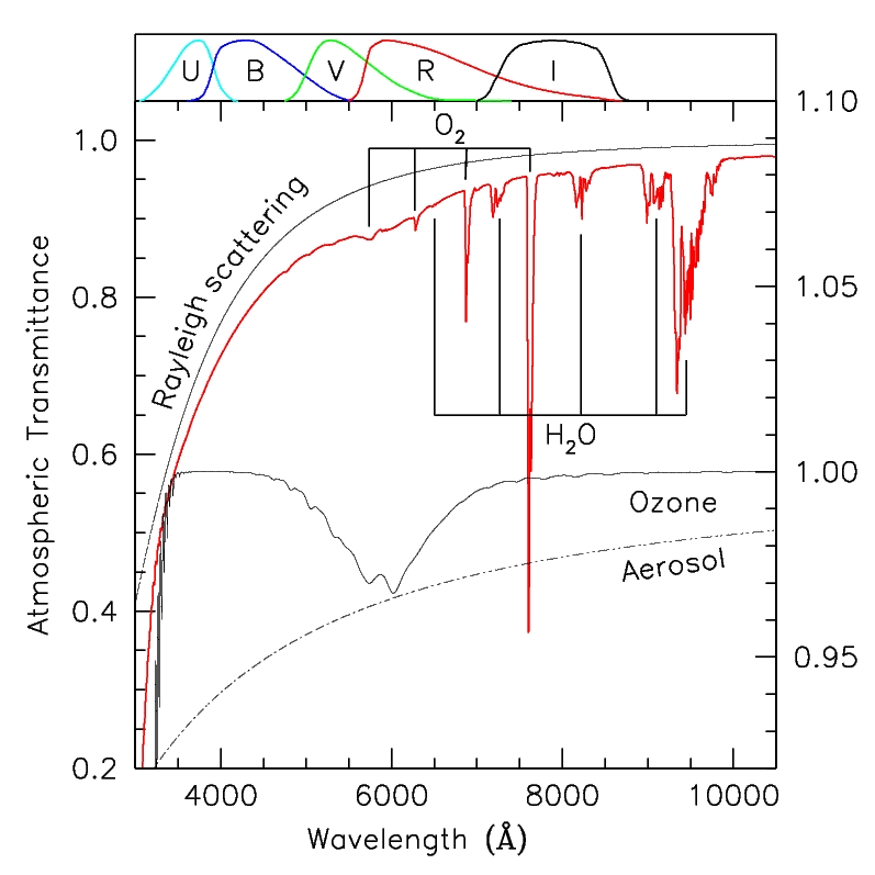
Figure 1: Model optical transmittance computed for Cerro Paranal with the LBLRTM code (see Sect. 5) for one airmass. The main extinction components are identified. The scale to the right refers to the ozone and aerosol components only. For presentation the model has been convolved with a Gaussian profile (FWHM=12 Å). The curves on the top panel trace the normalised $UBVRI$ Johnson-Cousins passbands.

Although several works have been published for two astronomical sites located in the Atacama Desert, i.e. La Silla (Tüg tug (1977); Sterken & Jerzykiewics sterken77 (1977); Rufener rufener (1986); Sterken & Manfroid sterken (1992); Grothues & Gochermann grot (1992); Burki et al. burki (1995)) and Cerro Tololo (Stone & Baldwin stone (1983); Gutiérrez et al. gutierrez82 (1982, 1986); Stritzinger et al. max (2005)), a systematic work for the site of Cerro Paranal (2640 m above sea level, 24.63 degrees South), hosting the ESO Very Large Telescope (VLT), was still missing. Broad-band $UBVRI$ extinction coefficients are routinely obtained at this observatory since the early phases of VLT operations (Patat patat03 (2003)), in the framework of quality control and instrument trending. In principle, as La Silla and Cerro Tololo are placed at similar elevations above the sea level and latitude, no significant differences are expected in the extinction wavelength dependency, so that so far the extinction curves for these two observatories have been widely used to correct the optical spectra obtained at Paranal. However, Cerro Paranal is situated much closer to the Pacific Ocean (12 km), and this might turn into a different composition of the tropospheric aerosols, resulting in a different extinction law.

Moreover, the extinction curves currently in use for these observatories were derived more than 15 years ago, before the two major eruptions of El Chichón (1982) and Pinatubo (1991), so that they are most likely outdated. The available broad-band data for Paranal are not sufficient to address these issues. Therefore, it was decided to undertake the PARanal Spectral Extinction Curve project (hereafter PARSEC), with the manifold aim of a) obtaining a spectroscopic function for the extinction correction of optical spectra, b) getting an estimate of the variability of the various extinction components in a time lapse free of major volcanic eruptions affecting South America, and c) setting a term of reference for future studies and trend analyses at this site. This is particularly important in the view of the construction of the European Extremely Large Telescope on Cerro Armazones, which is located only 30 km away from Cerro Paranal. In this article we present the results of the PARSEC project, which was carried on between October 2008 and March 2009.

Very briefly, the optical extinction can be described by three separate components (Hayes & Latham hayes (1975)): Rayleigh scattering by air molecules, aerosol scattering, and molecular absorption (O₂, O₃ and H₂O). The contribution of the various components is illustrated in Fig. 1, where we present the transmittance computed for Paranal using the LBLRTM code (Clough et al. clough (2005)). While the Rayleigh scattering and aerosols act at all wavelengths, the effect of ozone in the optical is limited to the so-called Chappuis bands (Chappuis chappuis (1880)) between 5000 and 7000 Å, and the Huggins bands (Huggins, huggins (1890)) below 3400 Å. The molecular bands of O₂ and H₂O are relevant only above 6500 Å.

Table 1: PARSEC Target Stars

Star Id. R.A. DEC. $V$ $B-V$ Sp. Type Ref. (J2000) (J2000) GD108 1 10:00:47.3 $-$07:33:31.2 13.56 $-$0.22 sdB 1 GD50 2 03:48:50.1 $-$00:58:30.4 14.06 $-$0.28 DA2 1 EG274 3 16:23:33.8 $-$39:13:47.5 11.03 $-$0.14 DA 2 BPM16274 4 00:50:03.2 $-$52:08:17.4 14.20 $-$0.05 DA2 3 EG21 5 03:10:31.0 $-$68:36:02.2 11.38 +0.04 DA 2 Feige110 6 23:19:58.4 $-$05:09:55.8 11.82 $-$0.30 DOp 1 GD71 7 05:52:27.5 +15:53:16.6 13.02 $-$0.25 DA1 4 Feige67 8 12:41:51.8 +17:31:20.5 11.81 $-$0.34 sdO 1 (1) Oke (oke (1990)); (2) Hamuy et al. (hamuy92 (1992)); (3) Bohlin et al. (bohlin90 (1990)) (4) Bohlin, Colina & Finleybohlin (1995)

2 Observations

2.1 Instrumental setup

All observations were carried out using the FOcal Reducer/low-dispersion Spectrograph (hereafter FORS1), mounted at the Cassegrain focus of the ESO-Kueyen 8.2 m telescope (Appenzeller et al. appenzeller (1998); Szeifert et al. szeifert (2007)). At the time of the observations discussed in this paper, FORS1 was equipped with a mosaic of two blue-optimised, 2048$\times$4096 15$\mu$m pixel (px) E2V CCDs. The spectra were obtained with the low-resolution G300V grism coupled to a long, 5.0 arcsec wide slit, giving a useful spectral range 3100–9330 Å, and a dispersion of $\sim$3.3 Å px^-1. The spatial scale along the slit is 0.252 arcsec px^-1. The G300V grism shows a rather pronounced second order contamination, starting at about 6100 Å (Szeifert et al. szeifert (2007)). To cover the widest possible wavelength range we run the observations using two setups, one with no filter (blue setting) and one with the order sorting filter GG435 (red setting). The latter provides a wavelength range free of second order contamination 4400–8100 Å.

The E2V detectors suffer from a marked fringing above 6500 Å (Szeifert et al. szeifert (2007)). This becomes extremely strong for $\lambda>$8000 Å, reaching a peak-to-peak amplitude of $\sim$20%, and it is not possible to remove it from the data. Therefore, the spectral region above this wavelength is practically unusable for our purposes.

Table 2: Log of the observations

GRISM 300V (blue setting) Star Number Time Range Nights Airmass distribution Id. of spectra (MJD-54000) 1.0–1.2 1.2–1.5 1.5–2.0 $>$2.0 1 104 761.4 – 922.0 28 35 17 36 16 2 76 743.4 – 811.3 18 14 31 15 16 3 44 848.4 – 921.4 16 29 11 4 0 4 38 751.1 – 811.2 3 12 10 9 7 5 17 745.4 – 750.4 6 0 0 17 0 6 11 751.3 – 784.2 2 3 0 3 5 7 12 794.4 – 805.4 4 0 0 9 3 8 3 879.4 – 879.4 1 0 0 3 0 Total 305 743.4 – 922.0 46 93 69 96 47 GRISM 300V + GG435 (red setting) 1 92 761.4 – 922.0 24 36 10 30 16 2 76 743.4 – 811.3 18 13 32 14 17 3 37 848.4 – 921.4 13 27 6 4 0 4 38 751.2 – 811.2 3 12 8 11 7 5 19 745.4 – 750.4 6 0 0 19 0 6 18 751.3 – 784.2 2 4 0 3 11 7 12 794.4 – 805.4 4 0 0 8 4 8 3 879.4 – 879.4 1 0 0 3 0 Total 295 743.4 – 922.0 43 92 56 92 55

2.2 Target selection and observations

In principle, there is no need to observe spectrophotometric standards for deriving the extinction curve, as any relatively bright star could be used for this purpose. However, observing standard stars has the advantage that the same data can be used also for the calibration plan purposes, hence mitigating the impact on normal science operations. For this reason, the programme stars were chosen among those included in the FORS1 calibration plan. To limit the strength of the Balmer photospheric absorption lines (which tend to hamper the derivation of the extinction curve, especially in the blue domain), preference was given to hot, blue objects. The selected target stars are listed in Table 1, which also presents their main properties. Exposure times ranged from five seconds to a minute for the faintest targets (i.e. GD50, BPM16274). Since the maximum shutter timing error across the whole field of view of FORS1 is $\sim$5 ms (Patat & Romaniello shutter (2005)), the photometric error associated to the exposure time uncertainty is 0.1% or better.

The spectroscopic data were collected on a time range spanning about 6 months, between October 4, 2008 and March 31, 2009. The target stars were observed randomly, mainly during morning twilight. On a few occasions the same star was observed several times during the same night, covering a wide range in airmass (hereafter indicated as $X$). In total, more than 300 spectra were obtained for each of the two setups, with $X$ ranging from 1.0 to 2.6. The exact number of data points, time and airmass ranges are shown in Table 2, together with the airmass distribution for each of the eight programme stars. The observations were carried out under photometric or clear conditions, which were judged at the telescope based on the zero-points delivered by the available imaging instruments (transparency variations $<$10% across the whole night in the $V$ passband). The quality of the nights was also checked a posteriori, using the data provided by the Line of Sight Sky Absorption Monitor (LOSSAM), which is part of the Differential Image Motion Monitor (DIMM) installed on Cerro Paranal (Sandrock et al. asm (2000)). For this purpose, we have retrieved the DIMM archival data for all relevant nights, and examined the RMS fluctuation of the flux of the star used by the instrument to derive the prevailing seeing. When this fluctuation exceeded 2% (or no LOSSAM data were available), the night was classified as non suitable, and the corresponding data rejected. Table 2 lists only data that passed this selection (600 out of 672 initial, non-saturated spectra).

Table 3: FWHM image quality distribution in PARSEC spectra.

$\lambda$ $s_{min}$ $s_{med}$ $s_{max}$ $s_{95}$ (Å) (arcsec) 3500 0.93 1.49 2.91 2.41 4500 0.60 1.05 2.68 1.97 7500 0.54 1.02 2.46 1.93

All spectra were obtained with the slit oriented along the N-S direction, which is strictly optimal only for observations close to the meridian. The misalignment between the slit and the parallactic angle at large hour angles (i.e. for targets at high airmass), can potentially lead to slit losses due to the differential atmospheric refraction (Filippenko flipper (1982)), and the seeing increase at larger zenith distances (Roddier roddier (1981)). As a consequence, the estimated extinction coefficient might be systematically overestimated. To minimise this effect we used a 5 arcsec wide slit for all observations; this, coupled to the typical seeing attained during our observations (see Table 3), ensures that differential light losses are negligible for all data taken at $X<$2. Additionally, FORS1 is equipped with a Linear Atmospheric Dispersion Corrector (LADC), which is capable of maintaining the intrinsic image quality down to airmass $\sim$1.5 (Avila, Rupprecht & Becker avila (1997)). At larger airmasses the LADC only partially reduces the effect of the atmosphere.

The image quality values (FWHM) reported in Table 3 were deduced directly from the data, analysing the profiles perpendicular to the dispersion direction at different wavelengths. The Table presents minimum ($s_{min}$), maximum ($s_{max}$), median ($s_{med}$) and 95-th percentile ($s_{95}$) of the observed image quality distribution. The image quality turns out to be better than $\sim$1.5 arcsec in 50% of the cases. While we did not attempt to account for the effects of atmospheric refraction, we have applied a correction for the slit losses caused by seeing. The method is described in Appendix A.

3 Data reduction

The data were processed using the FORS Pipeline (Izzo, de Bilbao & Larsen izzo (2009)). The reduction steps include de-bias, flat-field correction, and 2D wavelength calibration. The spectra were then extracted non-interactively using the apall task in IRAF after optimizing the extraction parameters. Because of the wide (5 arcsec) slit used to minimise flux losses, the uncertainty in the target positioning within the spectrograph entrance window is expected to produce significant shifts in the wavelength solution. For this reason, for each standard star we selected a low-airmass template spectrum (drawn from the data sample), to which we applied a rigid shift in order to match O₂ and H₂O atmospheric absorption bands. Then, the shift to be applied to each input spectrum was computed via cross correlation to the corresponding template spectrum. For doing this we first subtracted the smooth stellar continuum estimated by the continuum task in IRAF. Wavelength shifts exceeding 10 Å ($\sim$3 px) were recorded during this process.

The RMS error of the wavelength solution is of the order of 1Å. Since the bluest line used by the FORS1 pipeline is He i 3888Å, systematic deviations at shorter wavelengths could in principle occur. To check this possibility, we inspected the calibration frames after applying to them the same wavelength solution used for the programme stars. Thanks to the enhanced blue sensitivity of the EEV detector, several lines (identified as Hg i 3650 Å, Cd i 3610 Å and Cd i 3466, 3468Å), are clearly detectable. The measured wavelengths of these features turn out to be within $\sim$3Å from their laboratory values, corresponding to $\sim$1/4 of the typical FWHM resolution. This indicates that the wavelength solution is accurate to within a few Å down to $\sim$3400 Å. To quantify the effect of wavelength calibration inaccuracies of this order, we derived the extinction curve applying a wavelength offset to the data. For an offset of $\pm$3.3 Å (one pixel), the variation is below $\mp$0.001 mag airmass^-1 in the red, while it reaches $\mp$0.003 mag airmass^-1 at the blue edge ($\sim$3400 Å).

Since the adopted slit width is much wider than the typical seeing characterizing our data set, the actual resolution in the spectra depends on the prevailing seeing conditions. While this has no appreciable influence on the smooth stellar continuum, Balmer lines are expected to be affected, especially in their cores. In principle, this can be mitigated by matching the resolutions of the input spectra by a Gaussian profile convolution. However, in sight of the targeted resolution of the extinction curve, which is several tens of Å (see Sect. 4), and the fact that different stars have distinct line profiles and depths anyway, we have not attempted to correct for this effect. As a consequence, weak spurious features are expected at the wavelengths corresponding to the strongest hydrogen lines, such as H$\alpha$ and H$\beta$.

During the PARSEC campaign, no instrument intervention or mirror re-aluminization has occurred, guaranteeing the homogeneity of the data. However, it is known that the main mirrors of the VLT are subject to a reflectivity loss, mainly due to aluminum oxidation. The losses are as large as $\sim$13% per year in the $U$ band, they decrease at redder wavelengths, and reach $\sim$5% per year in the $I$ band (Patat patat03 (2003)). Since the data presented in this paper span over six months, the implied efficiency variation is significantly higher than the measurement errors, and this is expected to increase the noise. To account for this effect, at least to a first order, the measured instrumental magnitudes were corrected using the time elapsed from the previous aluminization (May 17, 2008; MJD=54603.5), and a linear interpolation of the values deduced from broad band photometry (Patat patat03 (2003)) to the required wavelengths. The application of this correction reduces the RMS scatter from the best fit solution by $\sim$25%.

Finally, airmasses were derived from the unrefracted zenith distances by means of the classical formula proposed by Hardie (hardie (1962)). We note that since $\sim$83% of the spectra were obtained at $X\leq$2, airmasses computed using other formulations discussed in the literature are always to within $\sim$0.001.

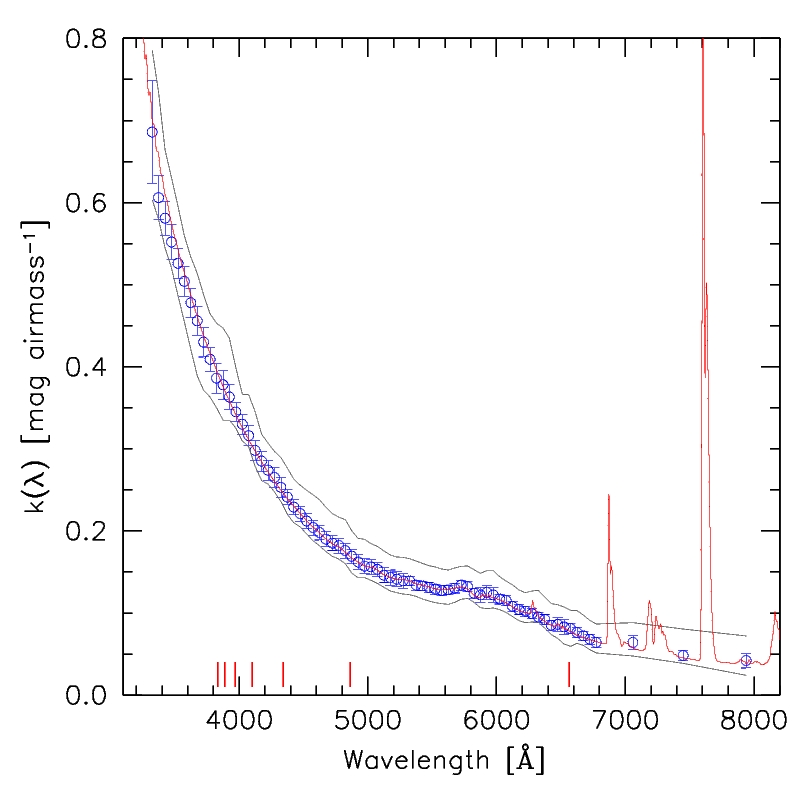
Figure 2: Best fit extinction coefficient for the blue (circles) and red (triangles) settings. The errorbars indicate the 3-sigma uncertainty of the best fit solution. The upper and lower grey curves trace the 95% variation level of single measurements. The solid curve is an LBLRTM simulation for Paranal (see Sect. 5), while the vertical segments at the bottom mark the positions of the first 7 Balmer lines.

4 Derivation of the extinction curve

The first step in the derivation of the extinction curve is the calculation of instrumental magnitude within predefined spectral bins. This is defined as follows:

$$m(\lambda)=-2.5\log\int_{\lambda-\Delta\lambda/2}^{\lambda+\Delta\lambda/2}s(\lambda)\;d\lambda$$

where $s(\lambda)$ is the observed spectrum (in electrons s^-1) and $\Delta\lambda$ is the spectral bin size. The fluxes within the bins were computed by numerical integration of the extracted, wavelength-calibrated spectra. In the following we will always consider bins of $\Delta\lambda$=50 Å (15 px). This choice is motivated by three reasons: a) the resulting resolution is sufficient to follow in great detail the behavior of the continuum extinction; b) since the bin width is significantly larger than the typical spectral resolution ($\sim$15 Å FWHM), the values measured within adjacent bins should be completely uncorrelated, and c) the resulting nominal signal-to-noise ratio per resolution element ranges from 100 to 1200 across the whole wavelength range covered by the observations (95% of the bins have a signal-to-noise ratio larger than 500). Since below $\sim$7000 Å all spectra are dominated by the object’s shot-noise, the precision of the instrumental magnitudes is of the order of 1% or better. Above this wavelength the dominant source of uncertainty is fringing, which reaches peak-to-peak amplitudes of $\sim$20%. This limits the usable range to wavelengths shorter than 8100 Å. The instrumental magnitudes were computed within adjacent bins up to 6800 Å. To mitigate the effect of fringing, at larger wavelengths we have selected three bins (having widths of 160, 200, and 200 Å), centred at 7060, 7450, and 7940 Å respectively, in order to avoid the O₂ and H₂O bands (Fig. 1).

Once the instrumental magnitudes are corrected for the efficiency degradation (see previous section) and slit losses due to bad seeing (see Appendix A), they can be used to finally derive the extinction curve.

Among all possible algorithms for combining data obtained for different programme stars, we opted for the global solution proposed by Hayes & Schmidtke (hs (1987)). This method is applicable to spectro-photometry and narrow-band photometry, i.e. when the passbands are nearly monochromatic, as is our case. Under these circumstances there are no colour-terms to be taken into account, and each wavelength bin can be treated independently from the others. One issue with this method is that, by construction, one cannot also solve for the zero-point of the linear relation at the same time that the slope (i.e. the extinction coefficient) is being determined. However, for our purposes this is not a problem, since we are only interested in the extinction term.

The result is presented in Fig. 2. As the values derived from the two settings in the intersection region (4400–6075 Å) are fully consistent within the estimated uncertainties, we averaged them. Also, we replaced the values corresponding to the strong Balmer lines with a linear interpolation between the adjacent bins. In Fig. 2 we also included the 95% confidence level deduced from the distribution of $k(\lambda)$ derived from each single observation (the extinction variations are discussed in more detail in Sect. 6).

5 Comparison with atmospheric model

To derive the basic physical parameters related to the extinction curve of Paranal we used the Line By Line Radiation Transfer Model (LBLRTM; Clough et al. clough (2005)). This code, based on the HITRAN database (Rothman et al. rothman (2009)), has been validated against real spectra from the UV to the sub-millimeter, and is widely used for the retrieval of atmospheric constituents. LBLRTM solves the radiative transfer using an input atmospheric profile, which contains the height profiles for temperature, pressure, and chemical composition. The code also includes the treatment of continuum scattering, and has an internal model for tropospheric aerosols (based on LOWTRAN).

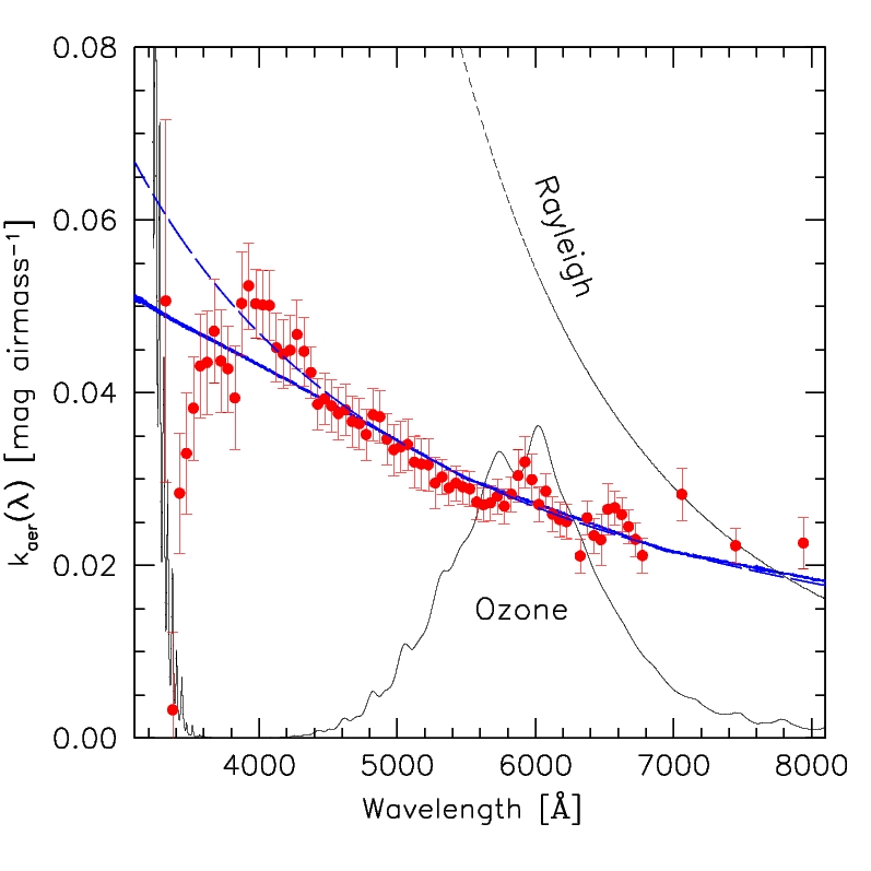
Figure 3: Aerosol extinction derived from the observed data and the LBLRTM model. The long-dashed line is a best fit model for $k_{\rm{aer}}(\lambda)$, with $k_{0}$=0.014 and $\alpha$=$-$1.42 (see text). Overplotted are also the Rayleigh (short-dashed), ozone (solid thin curve), and clean tropospheric aerosol (thick solid) components computed by LBLRTM (see text).

For the atmospheric profiles we adopted a standard equatorial profile as a basis for all calculations. To make the simulations more realistic we then replaced the standard profiles of pressure, temperature, and water content with an average vertical profile derived from the Global Data Assimilation System (GDAS). The average profile, provided to us by W. Kausch and M. Barden (Kausch & Barden 2010, private communication), was obtained averaging GDAS data over the last 6 years for the Paranal site. The corresponding amount of precipitable water vapor (PWV) is 2.0 mm, while the ozone column density is 238.8 Dobson Units (DU). Vacuum wavelengths were converted into air wavelengths using the relation derived by Morton (morton (1991)).

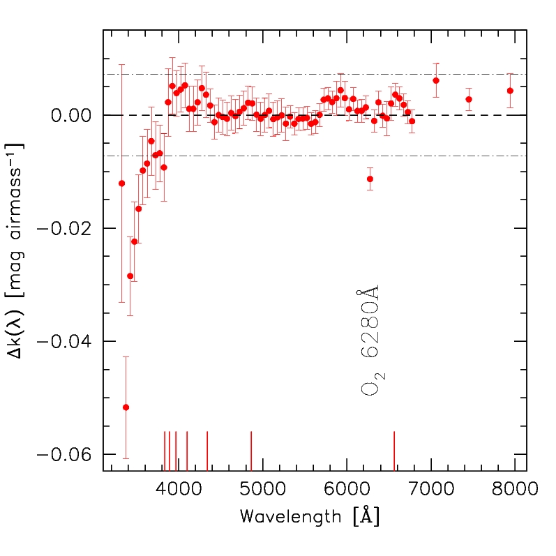
Figure 4: Deviations of the derived extinction curve from the LBLRTM simulation for Cerro Paranal (observed minus model). Errorbars are at the 1-sigma level. The deviation seen at about 6300 Å corresponds to the weak O₂ absorption peaking at $\sim$6280 Å. The dotted-dashed lines indicate the 3-sigma deviation from the best fit solution in the range 4000–6800 Å ($-$0.007 mag airmass^-1). The vertical segments at the bottom mark the positions of the first 7 Balmer lines.

Following Hayes & Latham (hayes (1975)), rather than assuming an aerosol model, we derived it from the data. For doing this we disabled the aerosol calculation in LBLRTM, and we computed the aerosol term $k_{\rm{aer}}(\lambda)$ as the difference between the data and the resulting model. The outcome is displayed in Fig. 3. As first suggested by Ångstrom (angstrom29 (1929, 1964)), the aerosol extinction can be described as $k_{\rm{aer}}(\lambda)=k_{o}\lambda^{-\alpha}$, where $k_{0}$ and $\alpha$ depend on the column density and size distribution of the aerosol mixture. This analytical formulation has been used in a number of extinction studies (Hayes & Latham hayes (1975); Angione & de Vaucouleurs angione (1986); Gutiérrez-Moreno et al. gutierrez82 (1982, 1986); Rufener rufener (1986); Minniti et al. minniti (1989); Burki et al. burki (1995); Mohan et al. mohan (1999); Schuster & Parrao schuster (2001)), and the typical value for $\alpha$ is $-$1.4$\pm$0.2 (with $\lambda$ expressed in $\mu$m; see for instance Burki et al. burki (1995)). This value is common for the so-called meteorological haze (i.e. free of volcanic pollutants) which characterises photometrically stable nights.

A reasonable fit to our data above 4000 Å is achieved for $k_{0}$=0.013$\pm$0.002 mag airmass^-1 and $\alpha=-$1.38$\pm$0.06. This result is fully in line with those found for other astronomical sites in the Atacama desert, like Cerro Tololo (Gutiérrez et al. gutierrez82 (1982)), and La Silla (Rufener rufener (1986); Burki et al. burki (1995)). However, the down-turn visible below 4000 Å is probably indicating a departure from a simple power-law model. We will get back to this issue while discussing the comparison with other observatories in the Atacama desert (Sect. 7). Although the properties of aerosols and the local conditions are difficult to model (Hess, Koepke & Schult hess (1998)), for the sake of completeness we plotted the LBLRTM clean tropospheric aerosol model in Fig. 3 (solid thick curve). In order to reach a reasonable fit we had to reduce by 25% the LBLRTM default aerosol column density in the first 10 km. Even larger reductions are necessary if one uses the marine or desert aerosol types implemented in the code.

To obtain information on the aerosol characteristics, we have used the Optical Properties of Aerosol and Clouds (OPAC) software package (Hess et al. hess (1998)). A best fit to the data above 4000Å indicates that the mixture is mostly composed by water soluble particles, with very low contamination by insoluble material, minerals and sea salt.

The final model for Paranal, obtained adding the best fit aerosol term to the LBLRTM results for the Rayleigh and ozone contributions, is plotted in Fig. 2, where it is compared to the data. The model reproduces very well the overall shape, and it also accurately follows the bumps in the 5800–6000 Å region related to the ozone component and O₂ (see Fig. 1). The quality of the match is better seen in Fig. 4, where we plot the residuals: the relative deviations are less than 0.01 mag airmass^-1 for the vast majority of the data. The largest discrepancies are seen redwards of 7000 Å, and bluewards of $\sim$4000 Å. While those in the red region are most likely explained by fringing, the deviations seen in the blue are more difficult to explain. Although most of the data points are formally consistent with a null deviation within a 3-sigma level, there is a clear trend which is suggestive of a systematic effect (see below, and the discussion in Sect. 7).

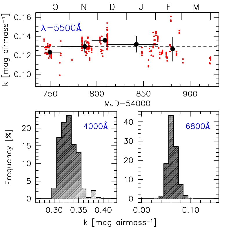
Figure 5: Upper panel: time evolution of the extinction at 5500 Å. The horizontal dashed line marks the best fit value. The large dots are the average values computed within the time intervals indicated by the horizontal bars. The vertical bars are the associated RMS deviations The time intervals include the same number of measurements (61), and the points are placed at the average time within each bin. Lower panel: distribution of the extinction coefficient at 4000 Å (left) and 6800 Å (right).

As far as the ozone content is concerned, we notice that the good fit achieved in the region of interest (5000 to 7000 Å) indicates this is, on average, as predicted by LBLRTM for the site location, i.e. $\sim$240 DU.

6 Extinction variability

An example of the extinction time evolution is presented in the upper panel of Fig. 5 for $\lambda$=6000 Å. Although there might be an hint of a mild modulation in the observed values (see the large dots in Fig. 5 and the discussion in Sect. 7), the limited time coverage of our sample ($\sim$6 months) does not allow us to firmly derive possible seasonal trends. Nonetheless, the available data are sufficient to study the extinction fluctuations under what can be considered as typical clear-sky conditions on Paranal.

6.1 Variability of continuum extinction

In general, the distribution of the extinction coefficient appears to be slightly skewed towards larger values, as found by several authors (see for instance Reimann, Ossenkopf & Beyersdorfer reimann (1992); Kidger et al. kidger (2003); Parrao & Schuster parrao (2003)). This is illustrated in the lower panel of Fig. 5, where we present the distributions for two different wavelengths (4000 and 6800 Å). The distribution appears to be broader in the blue than in the red. The peak-to-peak variations at the 95% level show a minimum value of 0.04 mag airmass^-1 at about 6000 Å, and grow to $\sim$0.07 mag airmass^-1 at 4000 Å. The inter-quartile range is $\sim$0.01 mag airmass^-1 for $\lambda>$4000 Å, while it reaches 0.04 mag airmass^-1 at the blue edge of the spectral range.

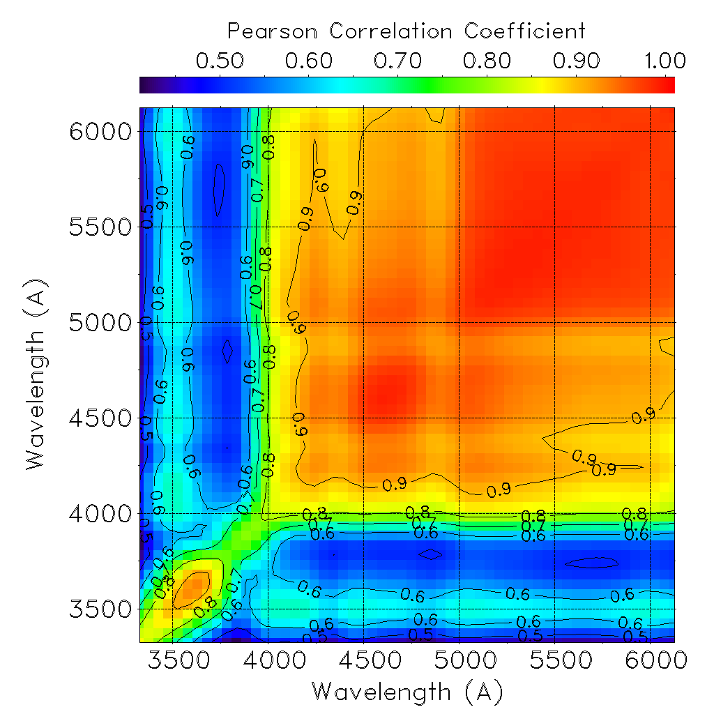
Figure 6: Extinction correlation map for the blue setting. The contours trace the iso-correlation levels. For presentation the map has been smoothed with a Gaussian filter ($\sigma$=75Å in both directions). The vertical and horizontal strips correspond to the Balmer lines. The decrease of correlation seen along the diagonal between 3700 and 4000 Å is due to the smoothing.

An important aspect is that the errorbars at various wavelengths are much larger than the scatter shown by the data points along the extinction curve (see Fig. 3). The explanation is that the estimated errorbars are dominated by overall variations of the extinction rather than by random errors. In order to show this behavior in a more quantitative way, we studied the correlation between the extinction measured within the different wavelength bins. Since, for any given spectrum, $k(\lambda)$ is measured exactly under the same conditions, this allows us to characterise the relation between the extinction variations across the whole spectral range covered by each of our setups separately. The result of this operation for the blue setting is presented in Fig. 6, which has been calculated using the Pearson coefficient $r_{xy}$ as a figure of merit for the correlation.

Two important facts emerge from this analysis. The first is that the correlation is strong ($r_{xy}>$0.8) above 4000 Å, implying that the various portions of the extinction curve tend to vary in unison, as expected in the case of changes in the aerosol content/composition. The second is that the extinction at $\lambda<$4000 Å appears to be less tightly correlated ($r_{xy}<$0.7) to that measured at larger wavelengths. We believe this is only partially due to the larger random errors, and it is caused by an independent behavior of the extinction curve below 4000 Å (see the discussion in Sect. 7). Although the correlation is always very significant above 4000 Å, it becomes weaker for $\lambda>$5700 Å, in the sense that the extinction in the red is less correlated with that measured below 5500 Å. One possible explanation for this is a combined effect of the independent variations in the aerosol (which affects all wavelengths), and in the ozone content (which mostly impacts the region between 5000 and 7000 Å).

Figure 7: Upper panel: distribution of aerosol extinction at 4000 Å. Lower panel: distribution of ozone extinction at 6000 Å. The upper scale indicates the corresponding ozone column density in DU (see text). The vertical dashed lines indicate the median, first and third quartile of the distributions.

6.1.1 Rayleigh scattering

During the nights used for the PARSEC project, the atmospheric pressure (retrieved from the Ambient Monitor, Sandrock et al. asm (2000)) showed a peak-to-peak excursion of 6.5 mb around the average value of 743.6 mb (RMS variation is 1.1 mb). Since the relative variation of the Rayleigh term is proportional to the relative variation of atmospheric pressure (see for instance Hansen & Travis hansen (1974)), this is expected to be constant to within 0.15% (RMS), with peak-to-peak fluctuations of less than 1%. Therefore, larger extinction variations can be attributed to changes in the aerosol content and, to a smaller extent and only within the wavelength range 5000–7000 Å, to variations in the stratospheric ozone column density (see Sect. 6.2.1).

6.1.2 Aerosol

To estimate the variability of the aerosol component, we have computed the residual extinction at 4000 Å (where the ozone contribution can be neglected), after subtracting the LBLRTM Rayleigh term to the blue setting data. The resulting distribution of the aerosol extinction, which we indicate as $k_{\rm{aer}}(4000)$, is presented in Fig. 7 (upper panel). The median value is 0.045 mag airmass^-1, and the semi-interquartile range is 0.009 mag airmass^-1. Only in $\sim$1% of the cases $k_{\rm{aer}}$ is smaller than 0.01 mag airmass^-1, while it can reach values larger than 0.10 mag airmass^-1 ($\sim$2.5%).

6.2 Variability of molecular bands

In the wavelength range covered by our observations, the most relevant absorption bands are from molecular oxygen (O₂ and O₃) and water. While the Chappuis bands of O₃ are important between 5000 and 7000 Å, O₂ and water mostly affect wavelengths larger than 6500 Å (see Fig. 1). In the following we briefly discuss the effect of their variability.

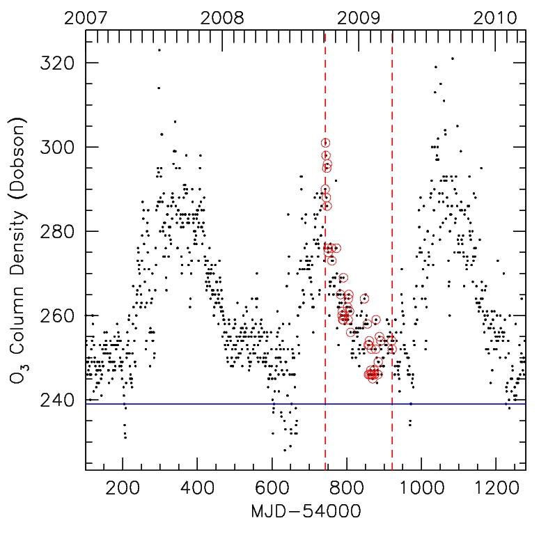
Figure 8: Ozone column density for the Paranal site measured by the Ozone Monitor Instrument on board of AURA. The two vertical dashed lines indicate the time range covered by PARSEC data. The circles mark the dates when PARSEC data were obtained.

6.2.1 Ozone bands

Ozone is the main responsible for the cutoff in the atmospheric transmittance below 3400 Å, where the O₃ component quickly surpasses the Rayleigh scattering (the ozone term reaches $\sim$2.5 mag airmass^-1 at 3000 Å). Since our data do no cover this wavelength region, we estimated the ozone column density measuring the extinction $k_{\rm{O}_{3}}$ corresponding to the peak of the Chappuis bands at $\sim$6000 Å (see Fig. 3). This was achieved removing the Rayleigh contribution (which was assumed to be constant in time), and an estimate of $k_{\rm{aer}}$ at 6000 Å. Since the aerosol is strongly variable, for each data set we have extrapolated the value measured at 4000 Å (cf. Sect. 6.1.2), conservatively assuming that $k_{\rm{aer}}$ follows the usual power law with $\alpha$=$-$1.38, so that $k_{\rm{aer}}(6000)\approx 0.6\;k_{\rm{aer}}(4000)$. The distribution of $k_{\rm{O}_{3}}$ is shown in Fig. 7 (lower panel). The average value is 0.039 mag airmass^-1 (0.002 mag airmass^-1 RMS), which is slightly larger than the LBLRTM prediction for Paranal (0.036 mag airmass^-1). The peak-to-peak variation is about 0.02 mag airmass^-1, and this would be sufficient to produce an enhanced extinction variability, at least at the Chappuis bands peak ($\sim$6000 Å). However, a significant fraction of the variance seen in the ozone extinction is most likely due to measurement errors, and uncertainties in the estimate of the underlying aerosol contribution.

Figure 9: Example spectrum of Feige 110 obtained with FORS1 on March 13, 2006 (grism G300I+OG590; airmass $X$=1.03). The signal-to-noise ratio per pixel on the continuum is $\sim$200. The main molecular absorption bands are marked. Superimposed are two LBLRTM simulations with PWV=2mm (dotted curve), and PWV=6mm (solid curve). In both cases the O₂ column density is 3.3$\times$10²⁴ cm^-2. Note that at the time this spectrum was obtained, FORS1 was equipped with a Tektronik detector much less affected by fringing.

To retrieve the implied ozone column density N(O₃), we have run a series of LBLRTM simulations scaling the O₃ profile to obtain a total N(O₃) between 60 and 480 DU. In this range $k_{\rm{O}_{3}}(6000)$ scales linearly with the column density, and a best fit to the model data gives the following relation:

$$k_{\rm{O}_{3}}(6000)\simeq 1.51\times 10^{-4}\;\mbox{N(O${}_{3}$)}$$

where $k_{\rm{O}_{3}}(6000)$ is expressed in mag airmass^-1, and N(O₃) is expressed in DU. From this we derive an average O₃ column density of 258 DU (the RMS deviation is 14 DU).

To cross-check this result, we run an independent analysis of the ozone variability using the satellite data provided by the Ozone Monitor Instrument (OMI) on board of NASA AURA. OMI derives the daytime ozone column density by comparing the amount of back-scattered solar radiation in the UV and in the optical. The OMI O₃ column density over Paranal collected between 2007 and 2009 clearly shows a seasonal trend (see Fig. 8), with maxima attained around August, September and October ($\sim$300 DU), and minima reached in February, March and April ($\sim$240 DU). The average value during the PARSEC campaign was about 260 DU, which is slightly larger than the value given by the LBLRTM model ($\sim$240 DU; see previous section). A closer inspection to the OMI data shows that the ozone content steadily decreased during the time covered by our observations. The peak-to-peak variation is about 25%. This turns into a maximum variation of $\sim$0.01 mag airmass^-1 at $\sim$6000 Å during the time covered by our observations. An inspection of the time evolution of $k_{\rm{O}_{3}}(6000)$ shows no traces of such a steady decrease, and the fluctuations appear to be dominated by short timescale variations, partially attributable to random errors.

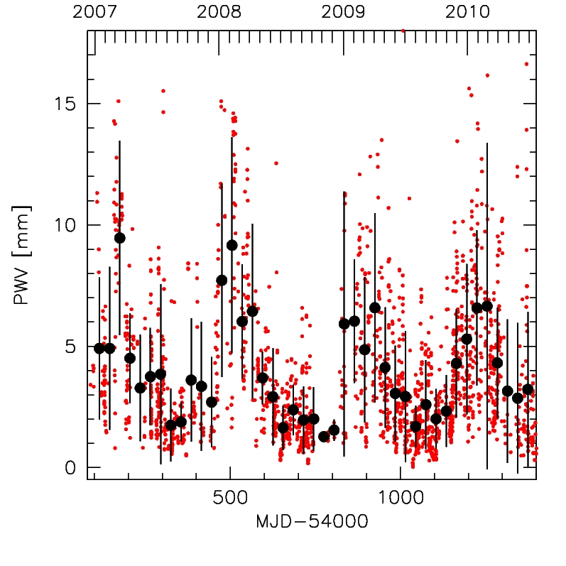
Figure 10: Precipitable water vapor measured in Paranal between 2007 and 2010 (Smette et al. smette (2007)). The large dots and error bars indicate the monthly averages and the associated RMS deviations, respectively.

6.2.2 Oxygen bands

Molecular oxygen shows two main O₂ vibrational absorption bands centred at 6870 Å and 7605Å, usually indicated as B and A bands, respectively (Fig. 9). Their typical equivalent widths (EW) are $\sim$6Å and $\sim$28Å, which make them easily detectable in low resolution spectra. To quantify the variability of O₂ column density, and its effect on the extinction, we have measured the EW of the B band in the red setting spectra. The A band is severely affected by fringing, and so no very accurate measurements were possible. However, the integrated strengths of the two bands are well correlated, as demonstrated by a series of LBLRTM simulations run for different values of the column density N(O₂). Additionally, they both follow a linear dependency on airmass, down to $X$=2.5.

The measurements clearly show the EW airmass dependency, which is well reproduced by the following best fit relation:

$$EW_{6870}=5.47\pm 0.04+(2.56\pm 0.06)\;(X-1)$$

where $EW_{6870}$ is expressed in Å. With the aid of this relationship one can correct the observed values to zenith, and derive the column density using a standard curve of growth procedure. For this purpose we computed a number of LBLRTM models varying N(0₂) between 8.4$\times$10²³ cm^-2 and 6.7$\times$10²⁴ cm^-2. Subsequently we measured the EW of the B band on the output spectra, after convolving them with a Gaussian profile to simulate the instrumental broadening (FWHM=12Å). A best fit using a second order polynomial gives the following result:

$$\log\mbox{N(O${}_{2}$)}=23.15+0.308\;EW_{6870}+0.013\;EW^{2}_{6870}$$

The zenith-corrected values of $EW_{6870}$ show a peak-to-peak range of 2.5Å, with an average value of 5.46Å (RMS=0.42Å). This corresponds to $\log\mbox{N(O${}_{2}$)}$=24.4 cm^-2 (2.5$\times$10²⁴ cm^-2), which is close to the value predicted by the LBLRTM model (24.52, or 3.3$\times$10²⁴ cm^-2). See also the match between the model and real data in Fig. 9. Incidentally, as proposed by Stevenson (stevenson (1994)), synthetic absorption spectra of this quality can be proficiently used to correct low resolution data for telluric features.

To evaluate the impact of O₂ variability on the extinction, we have run a series of LBLRTM models for different values of N(O₂) within the range deduced from the data. Although the variation in EW is significant (45% peak-to-peak), the effect remains confined to the two strong bands. The extinction coefficient variation is less than 0.01 mag airmass^-1 in $R$ and $I$, while no measurable effect is seen in $U$, $B$ and $V$ passbands. The total contribution of O₂ to the broad-band extinction is 0.01 and 0.03 mag airmass^-1 in $R$ and $I$, respectively, while it is below 0.002 in all other pass-bands.

As far as the time evolution is concerned, the data show short timescale variations (cf. Sect. 6.3), while there is no statistically significant signature of a long term trend over the six months spanned by our observations. Also, a correlation analysis between the EW of O₂ and the extinction coefficient derived on each single spectrum in the red setting had shown that these are completely independent ($r_{xy}<$0.2), irrespective of the wavelength under consideration.

6.2.3 Water bands

In the optical there are three bands that contribute to the extinction, at 7200, 8200 and 9400 Å, the latter being the most prominent one (Fig. 1) and affecting the $z$ passband. The intensity of these absorption bands is well correlated to the Precipitable Water Vapor (PWV), so that a best fit using an appropriate radiation transfer model and suitable vertical profiles enables the retrieval of the PWV amount directly from observed high-resolution spectra (see for instance Smette, Horst & Navarrete smette (2007)). A similar method can be used to roughly estimate the PWV from the global EW of a given water band measured on low resolution spectra. This can be then translated into H₂O column density, and finally converted into PWV. An example is shown in Fig. 9, which illustrates the very good match between the data and an LBLRTM model with PWV=6mm. Using LBLRTM simulations run with different values of water column density, we have derived the following relation for the band at 7200 Å, which holds for PWV$\leq$10 mm:

$$PWV\approx 0.4\;EW_{7200}+0.01\;EW^{2}_{7200}$$

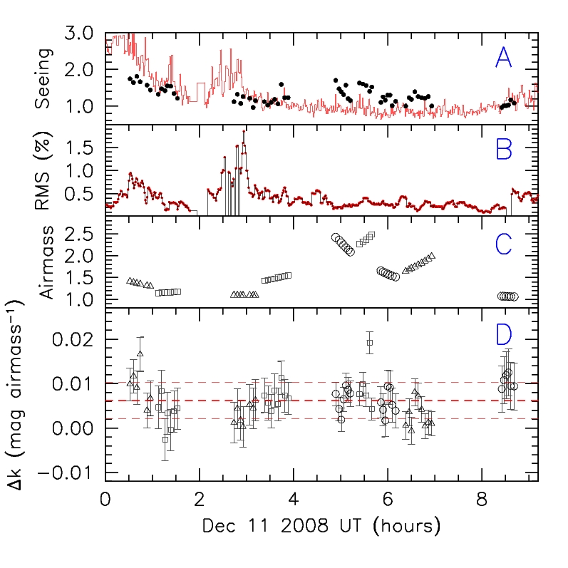
Figure 11: Short timescale variations observed on Dec 11, 2008 at 5000 Å. Panel A: DIMM seeing (the dots indicate the image quality measured on the spectra). Panel B: LOSSAM RMS fluctuations. Panel C airmass. Panel D: deviations from the average extinction at 5000 Å. Different symbols refer to different stars: GD108 (circles), GD50 (triangles), and BPM16274 (squares). The horizontal dashed lines trace the average deviation (middle) and $\pm$1 sigma levels (upper and lower).

Before entering the EW values into this relation, one needs to correct to zenith the values measured at airmass $X$. This can be done through the following formula, which was derived from a series of LBLRTM simulations:

$$EW_{0}=EW(X)-3.59\;(X-1)$$

In principle, provided that the signal-to-noise on the continuum is sufficient ($>$50 per pixel), this relation can be used to retrieve the amount of PWV from low resolution optical spectra. For PWV=2mm, which is a typical value for Paranal (see below), it is $EW_{7200}$=4.1Å. Unfortunately, due to the severe fringing, and the relative weakness of the feature, we could not directly measure the amount of PWV in our spectra. Therefore, to estimate the variability of water features in the optical domain and its impact on extinction, we used the PWV data obtained on Paranal (Smette et al. smette (2007)) during 2008 and 2009. The PWV shows a strong seasonal dependency (see Fig. 10), with peak values exceeding 15mm in February–March. The distribution has a median value of 2.6, and in 95% of the cases is PWV$<$10 mm.

Variations in the amount of PWV have a mild effect on the extinction coefficients, and this is limited to $R$ and $I$ passbands only. The synthetic broad-band coefficients deduced from LBLRTM simulations increase by 0.01 and 0.02 mag airmass^-1 in $R$ and $I$ respectively, if PWV changes from 2mm to 10mm.

6.3 Short timescale variations

The PARSEC data were collected with the aim of giving a statistically robust description of Paranal extinction. Therefore, observations have been spread as much as possible across the six months range covered by the project. However, on a few occasions, the same standard stars were observed at different airmasses during the same night, hence enabling the the calculation of the specific night extinction, and the study of its variability on the scales of tens of minutes. The best data set was obtained on Dec 11, 2008, and it contains a number of repeated observations of GD108, GD50, and BPM16274. The data, spanning almost the whole duration of the night, are presented in Fig. 11 for $\lambda$=5000 Å.

The extinction (on average 0.006 mag airmass^-1 higher than the best fit value 0.157$\pm$0.003), shows an RMS variation of 0.004 mag airmass^-1, which is comparable to the typical measurement error. Judging from the DIMM intensity fluctuations (Fig. 11, panel B), the night was stable, with RMS flux fluctuations at 5000 Å below 1.5% on the scale of one minute. This is indeed reflected on the stability of the extinction, which appears to vary by a similar amount. We also notice that data taken at high airmass do not show a systematic bias towards larger extinctions.

7 Discussion

The average extinction curve of Paranal, presented here for the first time, appears to conform to the expectations for the site. However, it is interesting to compare it to the data obtained for other two major observatories in the Atacama desert, i.e. Cerro Tololo (2200 m a.s.l.) and La Silla (2400 m a.s.l.), which are located within about 600 km from Paranal. The comparison is presented in Fig. 12. The data for Cerro Tololo are taken from the atmospheric extinction file ctioextinct.dat included in IRAF (Stone & Baldwin stone (1983); Baldwin & Stone baldwin (1984)). For La Silla we used the table published in Schwarz & Melnick (esomanual (1993)), who reported data obtained by Tüg (tug (1977)). These data are included in the atmoexan table of the MIDAS distribution.

While Paranal and Cerro Tololo display similar behaviors (but see the discussion below), La Silla shows a systematically lower extinction with the maximum deviation ($\sim$0.05 mag airmass^-1) occurring at about 4000 Å. Interestingly, the La Silla extinction curve is very well matched by an LBLRTM simulation with no aerosols (Fig. 12, dotted line). These exceptionally low values were noted already by Tüg, who had derived a maximum aerosol contribution of 0.01–0.02 mag airmass^-1 (see also Minniti et al. minniti (1989) for a comparison with two Argentinian sites). Since the extinction curve for La Silla was derived using data collected between 1974 and 1976, one possible explanation is that the transparency conditions have degraded in the Atacama desert in the last 35 years.

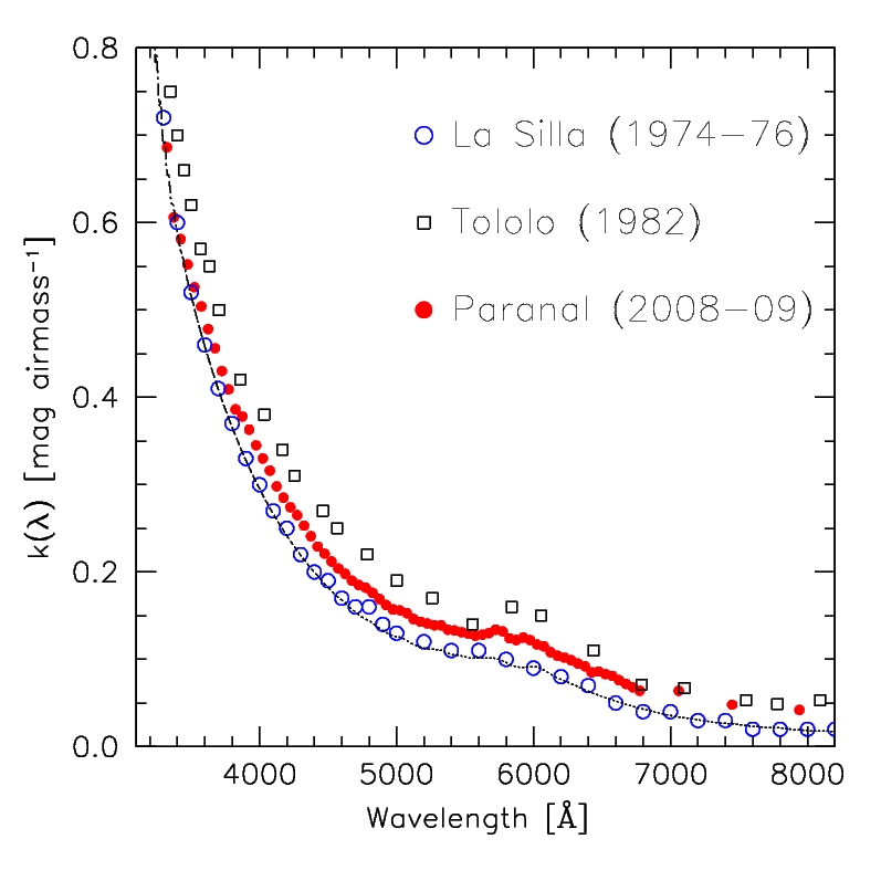
Figure 12: Comparison between the extinction curves of Paranal (this work), La Silla (Tüg tug (1977)), and Cerro Tololo (Stone & Baldwin stone (1983)). For comparison, the dashed curve traces a LBLRTM model computed for La Silla without aerosols.

Although it must be noticed that the extinction curve of La Silla was obtained selecting only the best nights (Tüg tug (1977)), the increased opacity is most likely due to a systematic change in the atmosphere above these sites. Already Stone & Baldwin (stone (1983)) had noticed this fact, and wrote that these observations indicate a non-grey increase of the extinction at Cerro Tololo, compared to values in use half a decade ago, averaging about 0.04 mag per airmass in the red and about 0.08 mag per airmass in the UV. In this respect it is important to note that the observations of Stone & Baldwin were most likely carried out before the volcanic eruption of El Chichón (March, April 1982), which severely affected the transparency at CTIO and La Silla (see Burki et al. burki (1995) for a comprehensive analysis).

But the most intriguing aspect shown by this comparison is the fact that while Paranal’s curve is very similar to the one of CTIO above 6500 Å, it gradually tends to the La Silla curve in the blue, so that they attain very similar values below 3800 Å (Fig. 12). The simplest explanation for this is a temporal evolution of the aerosol mixture above the Atacama desert.

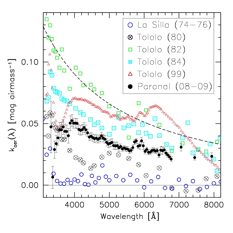
Figure 13: Comparison between the aerosol extinction in La Silla (1974–1976: Tüg tug (1977)), Cerro Tololo (1980: Gutiérrez-Moreno et al. gutierrez82 (1982); 1982: Stone & Baldwin stone (1983); 1984: Gutiérrez-Moreno et al. gutierrez86 (1986); 2004: Stritzinger et al. max (2005)), and Cerro Paranal (this work). The dashed line traces the $k_{aer}=k_{0}\lambda^{-\alpha}$ best fit law to the Cerro Tololo 1982 data ($k_{0}$=0.025 mag airmass^-1, $\alpha$=$-$1.4).

To test this hypothesis, we collected a number of published spectroscopic extinction curves obtained on different epochs between 1974 and 2009. Then we computed the pure aerosol contribution as we did in Sect. 5. The result is presented in Fig. 13. As expected, the 1974–1976 La Silla extinction curve (Tüg tug (1977)) shows an aerosol contribution which is smaller than 0.01 mag airmass^-1. Then, the data obtained at Cerro Tololo in July–August 1980 (Gutiérrez-Moreno et al. gutierrez82 (1982)) show a clear increase in the aerosol extinction, especially in the blue domain, where it reaches 0.05 mag airmass^-1. This increase becomes more marked in the next data set, obtained at Cerro Tololo in 1982 (Stone & Baldwin stone (1983)), as we said presumably before the El Chichòn eruption. The aerosol extinction is $\sim$0.07 mag airmass^-1 at 5000 Å, and exceeds 0.10 mag airmass^-1 below 4000 Å. The wavelength dependency is well reproduced by a power law with $k_{0}$=0.025 mag airmass^-1, and $\alpha=-$1.4 (see Sect. 5), as is typical of atmospheric haze (Burki et al. burki (1995)).

The next curve was obtained averaging the four data sets obtained at Cerro Tololo on January, April, May and July 1984 (Gutiérrez-Moreno et al. gutierrez86 (1986)), i.e. about 2 years after the El Chichòn eruption. Although the data above 6000 Å are a bit noisy, it is clear that while the extinction in the red remained at levels comparable to those measured in 1982, it decreased in the blue, making the wavelength dependency significantly shallower. This is usually interpreted as due to the evolution of the average particle size to larger values (see for instance Schuster & Parrao schuster (2001)).

The subsequent major volcanic event was the eruption of Pinatubo, which took place in June 1991. This produced very clear consequences on the extinction (Grothues & Gochermann grot (1992); Burki et al. burki (1995); Schuster & Parrao schuster (2001); Parrao & Schuster parrao (2003)). Since then, a number of intermediate size events took place, none reaching the level of the Pinatubo event. The most relevant for our study is the explosive eruption of Chaiten (Southern Chile, May 2008). However, at variance with those of El Chichón and Pinatubo, Chaiten produced a very small amount of SO₂, which is the main contributor to aerosol pollution. For this reason we tend to exclude this eruption had major effects on the atmosphere above the Chilean astronomical sites. In this respect we note that an enhancement in the SO₂ content can be also produced by local volcanoes that are not erupting, but many of which have strong vapor vents. These may have variations in intensity of activity that are not regularly monitored or observed.

The most recent extinction curve for the Atacama desert has been published by Stritzinger et al. (max (2005)), and it was obtained from data taken at CTIO on seven nights in February 1999. The resulting aerosol term shows a rather complex behavior, with a rapid decrease above $\sim$6400 Å, a rather flat plateau between 4000 and 6400 Å, and a drop followed by a rapid increase below 4000 Å (Fig. 13). Although some of the wiggles might be generated by the procedure used to derive the curve, the overall wavelength dependency is certainly different from the one expected for a typical atmospheric haze.

The deviation from an ordinary aerosol law is confirmed by our data set, which follows rather well (although with a shift of $\sim$0.01 mag airmass^-1) the points obtained at CTIO in 1984 (Gutiérrez-Moreno et al. gutierrez86 (1986)), with one remarkable difference, i.e. the downturn below 4000 Å. A similar drop has been observed by Schuster & Parrao (schuster (2001)) in their data obtained at S. Pedro Mártir about one year after the Pinatubo eruption. Small or even negative power indexes have also been reported by Sterken & Manfroid (sterken (1992)) and Burki et al. (burki (1995)) as typical of volcanic pollutants. We finally note that the curve by Stritzinger et al. (max (2005)) also shows a downturn in the blue, very similar to that displayed by the Paranal data. Parrao & Schuster (parrao (2003)) have interpreted this UV drop as a possible evidence for a masking (or decrease) of the normal atmospheric opacity produced by the presence of volcanic aerosols (see also the discussion in Sterken & Manfroid sterken (1992)). In addition, this might also be the signature of a more complex, possibly bi-modal, extinction law for the volcanic contribution (Parrao & Schuster parrao (2003)).

What is surprising about these results is that such anomalous wavelength dependencies are found almost twenty years after the Pinatubo event, when one would expect the atmospheric transmittance to be back to normal. But, as a matter of fact, the exceptional values recorded in La Silla in the 1970s were never observed again. The data collected in La Silla between 1974 and 1995 clearly show that in the almost ten years that separated El Chichòn and Pinatubo eruptions, the $UBV$ extinction never reached the levels preceding the first event (see Fig. 3 in Burki et al. burki (1995), and Schwartz schwartz (2005)). The extinction data presented in this work are on average $\sim$0.01 mag airmass^-1 lower than those measured at CTIO about two years after the El Chichòn eruption (Gutiérrez-Moreno et al. gutierrez86 (1986)), and $\sim$0.03 mag airmass^-1 lower than those published by Stritzinger et al. (max (2005)) for the same observatory. This might be the signal that the atmospheric transparency is slowly approaching the high values observed prior to the great eruptions that took place at the end of last century.

Further measurements in the next years will be needed to confirm the trend observed so far.

8 Conclusions

In this paper we presented the best fit extinction curve for Cerro Paranal, obtained combining spectroscopic data collected over more than 40 nights between October 2008 and March 2009. The main results of our analysis can be summarised as follows:

• Above 4000Å the curve is well fitted by an atmospheric model in which the aerosol is described by a power law of the form $k_{0}\;\lambda^{\alpha}$. Below this wavelength the data show a systematic deficit in the extinction, which exceeds $\sim$0.03 mag airmass^-1 at 3700 Å. Although this needs to be investigated with further observations, it may indicate the presence of pollutants of volcanic origin in the atmosphere above the Atacama desert.

• During the six months covered by our observations, the extinction distribution is characterised by a semi-interquartile range of 0.01 mag airmass^-1 above 4000 Å, with peak-to-peak variations up to $\sim$0.1 mag airmass^-1 in the UV.

• While the extinction measured at the various wavelengths is well correlated above 4000 Å, the correlation is much weaker below this limit. This supports the conclusion that the UV portion of the aerosol contribution follows an independent behavior.

• During the observing campaign, the Rayleigh scattering component was stable to $\sim$0.2% (RMS). The much larger extinction fluctuations, seen at all wavelengths and reaching peak values exceeding 0.1 mag airmass^-1 are attributable to changes in the aerosol amount and (possibly) composition. The median value of the aerosol contribution at 4000 Å is 0.05 mag airmass^-1.

• Ozone was found to vary by $\sim$5% (RMS) around an average value of 258 DU, in good agreement with that derived from the OMI data (260 DU).

• Although the O₂ A and B bands were found to vary by about 45%, the effect on the variation of broad-band $R$ and $I$ extinction coefficients is smaller than 0.01 mag airmass^-1. The column density of O₂ derived from the data is fully consistent with the LBLRTM prediction. No seasonal effect was detected.

• In the last 35 years the extinction above the Atacama desert has shown a marked evolution, most likely due to the two major eruptions of El Chichón and Pinatubo. The exceptionally low aerosol content measured in La Silla in 1974–76 was never re-established, indicating that it probably takes several decades before the pollutants completely fall out.

• The usage of the IRAF extinction curve ctioextinct.dat leads to systematic flux overestimates of more than 4% below 4000 Å. Also, it tends to over-correct by $\sim$0.03 mag airmass^-1 at about 6000 Å, which corresponds to the ozone bump. On the other hand, the usage of the atmoexan MIDAS table produces systematic flux underestimates that amount to $\sim$2% at 8000 Å, and exceed 5% at 4000 Å.

• The adoption of the best fit curve presented in this paper for the extinction correction of spectroscopic data obtained at Paranal under clear-sky conditions leads to an RMS uncertainty of about 1%.

Appendix A Correction for slit losses due to seeing

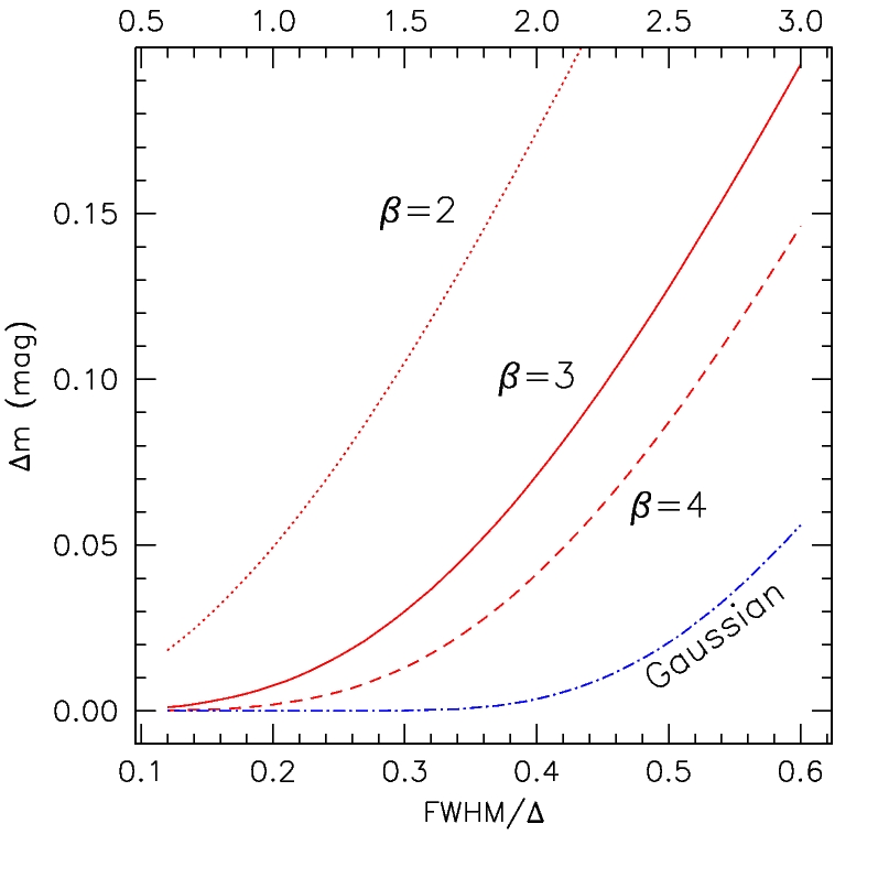
Figure 14: Slit losses for Moffat PSFs with different $\beta$ values. For comparison, the Gaussian case is also plotted (dotted-dashed line). The upper scale indicates the FWHM seeing (in arcsec) for a slit width $\Delta$=5 arcsec.

Because of the extended wings of the point spread function (PSF) typically delivered by telescopes, and depending on the slit width $\Delta$ used for the observations, a fraction of the incoming flux does not enter the spectrograph. If this loss were constant, there would be no effect on the final estimate of the extinction coefficients. However, data are obtained under different seeing conditions, and seeing tends to be larger at larger airmasses. Therefore, this introduces a systematic effect which leads to artificially higher extinction estimates. Obviously, these losses cannot be reduced by placing the slit along the parallactic angle or observing through an atmospheric dispersion corrector.

In this section we describe the method we have used to correct the instrumental magnitudes derived from our spectra. For this purpose, let us introduce a coordinates reference system placed on the focal plane of the telescope, with its origin on the optical axys. Then let us indicate with $P(x,y)$ the PSF, normalised so that:

$$\int_{-\infty}^{+\infty}\int_{-\infty}^{+\infty}P(x,y)\;dx\;dy=1$$

If the slit width is $\Delta$, then the slit flux losses (expressed in magnitudes) can be computed as:

$$\Delta m=-{\mbox{2}.5}\log\int_{-\infty}^{+\infty}\int_{-\Delta/2}^{+\Delta/2}P(x,y)\;dx\;dy$$ (1)

for any PSF profile. For our calculations we adopted the profile derived by Moffat (moffat (1969)):

$$P(x,y)=\left[1+\frac{x^{2}+y^{2}}{\sigma^{2}}\right]^{-\beta}$$

where the width parameter $\sigma$ is related to the FWHM as follows:

$$\sigma=\frac{FWHM}{2\sqrt{2^{1/\beta}-1}}$$

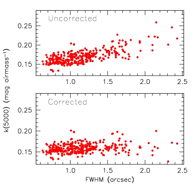
Figure 15: Effect of the slit losses correction on the PARSEC extinction at 5000 Å. Upper panel: original data. Lower panel: corrected data.

The typical values of $\beta$, deduced from observed stellar profiles, range between 2.5 and 4.0 (Saglia et al. saglia (1993)). For our calculations we have used $\beta$=3, which gives a very good fit to the VLT FORS1 data in the wavelength range of interest (3300–8000 Å). Equation 1 can be integrated numerically for different values of the FWHM, and the correction $\Delta m$ readily derived. A real example is illustrated in Fig. 14. For a slit width of 5 arcsec (as is our case), with a seeing of 1 arcsec the losses amount only to $\sim$0.008 mag, but they grow to $\sim$0.07 mag for a seeing of 2 arcsec.

The effect of the correction is illustrated in Fig. 15, which presents the PARSEC extinction data at 5000 Å. The uncorrected data show a clear dependency of $k$ from the seeing (the Pearson correlation factor is $r_{xy}$=0.71), while the corrected values show no correlation ($r_{xy}$=0.21). Since the seeing grows as $\lambda^{-1/5}$ (Roddier roddier (1981)), slit losses are higher in the blue than in the red. Therefore, not only does one expect a correlation between the uncorrected instrumental magnitudes and the seeing, but also that this relation becomes steeper in the blue. This expectation is confirmed by our data. An inspection of the PARSEC data at various wavelengths shows that the application of the correction removes any dependency of $k$ from seeing and airmass. As a side effect, it also reduces the spread of the data points.

Appendix B Tabulated extinction curve for Paranal

Table 4: Best fit extinction curve for Paranal

$\lambda$ $k(\lambda)$ $\sigma_{k}$ $\lambda$ $k(\lambda)$ $\sigma_{k}$ $\lambda$ $k(\lambda)$ $\sigma_{k}$ 3325 0.686 0.021 4625 0.198 0.003 5925 0.125 0.003 3375 0.606 0.009 4675 0.190 0.003 5975 0.122 0.003 3425 0.581 0.007 4725 0.185 0.003 6025 0.117 0.002 3475 0.552 0.007 4775 0.182 0.003 6075 0.115 0.002 3525 0.526 0.006 4825 0.176 0.003 6125 0.108 0.002 3575 0.504 0.006 4875 0.169 0.003 6175 0.104 0.002 3625 0.478 0.006 4925 0.162 0.003 6225 0.102 0.002 3675 0.456 0.006 4975 0.157 0.003 6275 0.099 0.002 3725 0.430 0.006 5025 0.156 0.003 6325 0.095 0.002 3775 0.409 0.005 5075 0.153 0.003 6375 0.092 0.002 3825 0.386 0.006 5125 0.146 0.003 6425 0.085 0.002 3875 0.378 0.006 5175 0.143 0.003 6475 0.086 0.003 3925 0.363 0.005 5225 0.141 0.003 6525 0.083 0.003 3975 0.345 0.004 5275 0.139 0.003 6575 0.081 0.002 4025 0.330 0.004 5325 0.139 0.002 6625 0.076 0.002 4075 0.316 0.004 5375 0.134 0.002 6675 0.072 0.002 4125 0.298 0.004 5425 0.133 0.002 6725 0.068 0.002 4175 0.285 0.004 5475 0.131 0.002 6775 0.064 0.002 4225 0.274 0.004 5525 0.129 0.002 7060 0.064 0.003 4275 0.265 0.004 5575 0.127 0.002 7450 0.048 0.002 4325 0.253 0.004 5625 0.128 0.002 7940 0.042 0.003 4375 0.241 0.003 5675 0.130 0.002 4425 0.229 0.003 5725 0.134 0.002 8500 0.032 (*) 4475 0.221 0.003 5775 0.132 0.002 8675 0.030 (*) 4525 0.212 0.003 5825 0.124 0.002 8850 0.029 (*) 4575 0.204 0.003 5875 0.122 0.003 10000 0.022 (*) (*) The last four values are interpolations from the LBLRTM model.

The merged extinction curve of Paranal is presented in Table 4. To allow the usage of the data across the whole optical domain, we have added four points obtained from the interpolation of an LBLRTM model. The wavelengths (8500, 8675, 8850, and 10000 Å) were selected to avoid the strong water absorption bands. The LBLRTM simulation was run disabling the aerosol calculation. Then we added the aerosol contribution using the best fit relation $k_{\rm aer}=k_{0}\lambda^{\alpha}$, with $k_{0}$=0.013 and $\alpha$=$-$1.38 (see Sect. 6.1.2).