On Dark Energy Isocurvature Perturbation

Abstract

Determining the equation of state of dark energy with astronomical observations is crucially important to understand the nature of dark energy. In performing a likelihood analysis of the data, especially of the cosmic microwave background and large scale structure data the dark energy perturbations have to be taken into account both for theoretical consistency and for numerical accuracy. Usually, one assumes in the global fitting analysis that the dark energy perturbations are adiabatic. In this paper, we study the dark energy isocurvature perturbation analytically and discuss its implications for the cosmic microwave background radiation and large scale structure. Furthermore, with the current astronomical observational data and by employing Markov Chain Monte Carlo method, we perform a global analysis of cosmological parameters assuming general initial conditions for the dark energy perturbations. The results show that the dark energy isocurvature perturbations are very weakly constrained and that purely adiabatic initial conditions are consistent with the data.

I introduction

Since the discovery of the accelerated expansion of the universe by observations of distant Type Ia supernovae (SNIa) in 1998 Riess:1998cb ; Perlmutter:1998np , dark energy has become a hot topic in physics and astronomy. So far a lot of models have been proposed in the literature. In general these models can be classified according to the equation of state (EoS) $w_{e}$ of the dark energy, defined as the ratio of its pressure to energy density. The simplest assumption is to consider dark energy with constant $w_{e}$, and more specifically to assume a cosmological constant whose EoS is equals to $-1$. Although this scenario is consistent with observationsJassal:2006gf , it suffers from the well-known fine-tuning and coincidence problemsweinberg ; CCproblem . Alternatively, dynamical dark energy models, such as quintessence Ratra:1987rm ; Wetterich:1987fm ; Caldwell:1997ii , phantom Caldwell:1999ew , k-essence ArmendarizPicon:2000dh , quintom Feng:2004ad ; Cai:2009zp and so on, have a time-dependent EoS. For quintessence $w_{e}\geq-1$, while for phantom $w_{e}\leq-1$. But for quintom models, the EoS crosses the boundary set by $w_{e}=-1$. To investigate dark energy without making use of specific field models, one often parameterizes the EoS of dark energy asChevallier:2000qy

$$w_{e}(a)=w_{0}+w_{a}(1-a)$$ (1)

where $a$ is the scale factor normalized to be 1 at the present time. We adopt this parametrization in the current work.

Given the fact that a lot of theoretical models exist in the literature, it is crucially important to use the accumulated high precision observational data from SNIa, the cosmic microwave background (CMB) radiation and large scale structure (LSS) surveys to constrain the value of $w_{e}(a)$. Since dynamical dark energy should fluctuate in space as described by the conservation of the energy-momentum tensor, in a global analysis with a general time evolving EoS one should take into account the dark energy perturbations in order to have a consistent procedure. This is particularly important when fitting cosmological parameters to the data of CMB and LSS. Simply switching off the dark energy perturbation is not theoretically correct and will lead to biased results. Numerically it has been shown that the results obtained are quite different between the two cases with and without the dark energy perturbations Bean:2003fb ; Mukherjee:2003rc ; Zhao:2005vj ; Xia:2005ge ; Weller:2003hw ; Xia:2007km ; Komatsu:2008hk ; Yeche:2005wn .

With the generally parameterized EoS, there inevitably exists a singularity when $w_{e}=-1$. When $w_{e}$ crosses this critical point, the dark energy perturbations will diverge Feng:2004ad ; Vikman:2004dc ; Hu:2004kh ; Caldwell:2005ai . It has been shown that in the context of general relativity, it is impossible to obtain a background which crosses the “cosmological constant boundary” with only a single scalar field or a single perfect fluid. In fact, this is the reason why the quintom scenario of dark energy needs to introduce extra degrees of freedom Feng:2004ad ; Vikman:2004dc ; Hu:2004kh ; Caldwell:2005ai ; Zhao:2005vj ; Li:2005fm ; xiaofei ; Lim:2010yk ; Deffayet:2010qz . In order to handle the perturbation when $w_{e}$ crosses $-1$, we proposed a method to deal with the dark energy perturbations during the crossing of the boundary $w_{e}=-1$ in Ref. Zhao:2005vj . According to this method, the energy and momentum density perturbations of dark energy are treated as constant during the small interval around the critical point $w_{e}=-1$. This method is justified in Ref. Li:2010hm from the viewpoint of general relativistic matching conditions.

Another issue concerned with the dark energy perturbations is the question of initial condition. Generally, there are two types of initial conditions for the perturbations: adiabatic and isocurvature. In Refs. Zhao:2005vj ; Xia:2005ge ; Xia:2007km ; Li:2010hm for the global fitting of the dark energy EoS to the observational data, it was assumed that the perturbations were purely adiabatic. In this paper we will study more general initial conditions which admit dark energy isocurvature perturbations and discuss the implications for CMB temperature and polarization power spectra and the LSS matter power spectrum. In the literature, baryon and dark matter isocurvature perturbations have been extensively discussed and tight constraints on these are obtained. There have also been studies of the dark energy isocurvature perturbations which, however, are usually limited in the framework of quintessence models Bucher:1999re ; Kawasaki:2001bq ; Malquarti:2002iu ; Moroipq ; Gordon:2004ez . In these studies, it has been shown that the quintessence isocurvature perturbations could lead to the suppression of the CMB quadrupole via the anti-correlation between the adiabatic and the isocurvature modesMoroipq ; Gordon:2004ez ; Li:2010ac ; Enqvist:2000hp . In this paper, working with the parameterized EoS, we consider both adiabatic and isocurvature initial conditions and the correlation between them in the likelihood data fitting analysis. We discuss the current constraints on the cosmological parameters, with result when admitting the possible existence of dark energy isocurvature modes. Our paper is organized as follows: in section II, we briefly review the theory of perturbations; In section III, we analytically study in detail the dark energy isocurvature perturbations; In section IV we study effects of the dark energy isocurvature perturbations on CMB and LSS, and we present the current constraints on them in Section V; Section VI is our summary.

II Adiabatic and Isocurvature perturbations

We consider a spatially flat Friedmann-Robertson-Walker universe as the background. The metric of the perturbed spacetime in the conformal Newtonian gauge reads,

$$ds^{2}=a(\eta)^{2}[(1+2\Phi)d\eta^{2}-(1-2\Phi)\delta_{ij}dx^{i}dx^{j}]~{},$$ (2)

where we have implicitly assumed that the shear perturbations can be neglected and the metric perturbations are fully described by one relativistic potential $\Phi$. In the matter sector, the perturbations are expressed by the perturbed energy-momentum tensor which is gauge dependent. However, for the discussions of perturbations on large scales it is more convenient to use gauge invariant variables constructed by combining the energy-momentum perturbations with the metric perturbations. In this paper, we use the following gauge-independent variables for each species

$$\zeta_{\alpha} = \frac{\delta_{\alpha}}{3(1+w_{\alpha})}-\Phi~{},$$

$$\Delta_{\alpha} = \frac{\rho_{\alpha}\delta_{\alpha}}{3}+\frac{\mathcal{H}}{k^{2}}(\rho_{\alpha}+p_{\alpha})\theta_{\alpha}~{},$$ (3)

where $\delta_{\alpha}\equiv\delta\rho_{\alpha}/\rho_{\alpha}$ is the density contrast, $\theta_{\alpha}\equiv ik^{i}\delta T^{0}_{~{}i\alpha}/(\rho_{\alpha}+p_{\alpha})$ is the corresponding momentum density perturbation, and the conformal Hubble parameter is defined by $\mathcal{H}=a^{\prime}/a$ with the prime denoting the derivative with respect to conformal time. $\zeta_{\alpha}$ is a comoving curvature perturbation, and as we will see later in this paper $\Delta_{\alpha}$ may be called an “effective” density perturbation. The conservation of the energy-momentum tensor at the linear order gives the equations governing the evolutions of $\zeta_{\alpha}$ and $\Delta_{\alpha}$:

$$\zeta_{\alpha}^{\prime}+3\mathcal{H}(c_{s\alpha}^{2}-c_{a\alpha}^{2})\frac{\Delta_{\alpha}}{\rho_{\alpha}+p_{\alpha}}+\frac{k^{2}}{3\mathcal{H}}(\frac{\Delta_{\alpha}}{\rho_{\alpha}+p_{\alpha}}-\zeta_{\alpha})=\frac{k^{2}}{3\mathcal{H}}\Phi~{},$$ (4)

$$\Delta_{\alpha}^{\prime}+(4\mathcal{H}-\frac{\mathcal{H}^{\prime}}{\mathcal{H}}+\frac{k^{2}}{3\mathcal{H}})\Delta_{\alpha}-(\mathcal{H}-\frac{\mathcal{H}^{\prime}}{\mathcal{H}}+\frac{k^{2}}{3\mathcal{H}})(\rho_{\alpha}+p_{\alpha})\zeta_{\alpha}=(\rho_{\alpha}+p_{\alpha})[\Phi^{\prime}+(2\mathcal{H}-\frac{\mathcal{H}^{\prime}}{\mathcal{H}}+\frac{k^{2}}{3\mathcal{H}})\Phi]~{}.$$ (5)

In the above equations, $c_{s\alpha}$ is the sound speed defined in the comoving frame of the fluid while the so-called adiabatic sound speed, $c_{a\alpha}$, is defined as $c_{a\alpha}^{2}\equiv p_{\alpha}^{\prime}/\rho_{\alpha}^{\prime}=w_{\alpha}-w_{\alpha}^{\prime}/[3\mathcal{H}(1+w_{\alpha})]$. For a perfect fluid $c_{s\alpha}=c_{a\alpha}$, and for a canonical scalar field $c_{s\alpha}=1$.

To close the system, we also need the Poisson equation,

$$\frac{k^{2}}{a^{2}}\Phi=-12\pi G\sum_{\alpha}\Delta_{\alpha}~{},$$ (6)

which can be obtained from the perturbed Einstein equations. Comparing this equation with the Poisson equation in the Newtonian gravity we can see that $\Delta_{\alpha}$ may be called an effective density perturbation. On super horizon scales $k\eta\ll 1$, the terms proportional to $k^{2}$ in Eqs. (4), (5) and (6) can be dropped, and these equations become

$$\zeta_{\alpha}^{\prime}+3\mathcal{H}(c_{s\alpha}^{2}-c_{a\alpha}^{2})\frac{\Delta_{\alpha}}{\rho_{\alpha}+p_{\alpha}}=0~{},$$ (7)

$$\Delta_{\alpha}^{\prime}+(4\mathcal{H}-\frac{\mathcal{H}^{\prime}}{\mathcal{H}})\Delta_{\alpha}-(\mathcal{H}-\frac{\mathcal{H}^{\prime}}{\mathcal{H}})(\rho_{\alpha}+p_{\alpha})\zeta_{\alpha}=(\rho_{\alpha}+p_{\alpha})[\Phi^{\prime}+(2\mathcal{H}-\frac{\mathcal{H}^{\prime}}{\mathcal{H}})\Phi]~{},$$ (8)

$$\sum_{\alpha}\Delta_{\alpha}=0~{}.$$ (9)

From equation (7), we see that for a perfect fluid $\zeta_{\alpha}$ is conserved on large scales.

To solve the set of perturbation equations, we need to specify the initial conditions. Usually these initial conditions are set at the time deep inside the radiation dominated era when the scales corresponding to observations today were far outside the horizon. Inflation provides a natural mechanism to generate these initial perturbations. They originate from quantum vacuum fluctuations and become classical perturbations when their corresponding length scales leave the horizon during inflation. In the post-inflation epoch, these primordial perturbations re-enter the horizon and interact with matter to cause the CMB anisotropies and structure formation. Hence it is important to inspect the evolutions of the perturbations on super-horizon scales until the scales re-enter the horizon. For this purpose we only need to consider the equations (7), (8) and (9). There are two types of solutions of these equations, called adiabatic and isocurvature (or entropy) modes. For adiabatic perturbation all comoving curvature perturbations $\zeta_{\alpha}$ are the same as that of radiation $\zeta_{r}$. The total comoving curvature perturbation is also equal to $\zeta_{r}$,

$$\zeta=\frac{1}{\rho+p}\sum_{\alpha}(\rho_{\alpha}+p_{\alpha})\zeta_{\alpha}=\zeta_{r}~{},$$ (10)

which is constant since $\zeta_{r}^{\prime}=0$. Thus, for adiabatic perturbation, the picture is simple: the primordial perturbations $\zeta$ are frozen while they are outside the horizon. With Eq. (9), the sum of Eq. (8) over all species gives

$$(\frac{\mathcal{H}^{\prime}}{\mathcal{H}}-\mathcal{H})\zeta=\Phi^{\prime}+(2\mathcal{H}-\frac{\mathcal{H}^{\prime}}{\mathcal{H}})\Phi~{}.$$ (11)

Integration of this equation gives

$$\Phi^{\rm adi}=C\frac{\mathcal{H}}{a^{2}}-\zeta_{r}(1-\frac{\mathcal{H}}{a^{2}}\int\frac{ada}{\mathcal{H}(a)})~{},$$ (12)

where $C$ is a constant. The first term on the right hand side decays in the expanding universe and can be neglected.

However, if one of the comoving curvature perturbations $\zeta_{\alpha}$ is not equal to $\zeta_{r}$, the density perturbation have an isocurvature mode. the isocurvature perturbation of species $\alpha$ is defined by

$$S_{\alpha}\equiv 3(\zeta_{\alpha}-\zeta_{r})=\frac{\delta_{\alpha}}{1+w_{\alpha}}-\frac{3}{4}\delta_{r}~{}.$$ (13)

In principle, if the universe contains $N$ components, there should be at most $N-1$ isocurvature density perturbations. With the presence of isocurvature modes, the equation (11) relating the potential and the total comoving curvature perturbation is still valid. However in this case $\zeta\neq\zeta_{r}$. If only one species $\alpha$ has isocurvature perturbation, $\zeta$ is

$$\zeta=\zeta_{r}+\frac{\rho_{\alpha}+p_{\alpha}}{3(\rho+p)}S_{\alpha}~{}.$$ (14)

It is not conserved on large scales. We may define $\xi_{\alpha}\equiv(\rho_{\alpha}+p_{\alpha})S_{\alpha}/3$, so that

$$\zeta=\zeta_{r}+\frac{\xi_{\alpha}}{\rho+p}~{},$$ (15)

and Eqs. (7) and (8) become

$$\xi_{\alpha}^{\prime}+3\mathcal{H}(1+c_{a\alpha}^{2})\xi_{\alpha}+3\mathcal{H}(c_{s\alpha}^{2}-c_{a\alpha}^{2})\Delta_{\alpha}=0~{},$$

$$\Delta_{\alpha}^{\prime}+(4\mathcal{H}-\frac{\mathcal{H}^{\prime}}{\mathcal{H}})\Delta_{\alpha}+(\frac{\mathcal{H}^{\prime}}{\mathcal{H}}-\mathcal{H})(1-\frac{\rho_{\alpha}+p_{\alpha}}{\rho+p})\xi_{\alpha}=0~{}.$$ (16)

The above equations describe how the isocurvature perturbations evolve on large scales and Eq. (14) or (15) characterizes the contribution of isocurvature perturbations to the total comoving curvature perturbation. The potential can be solved by integrating Eq. (11) and we obtain

$$\Phi=\Phi^{\rm adi}-4\pi G\frac{\mathcal{H}}{a^{2}}\int\xi_{\alpha}\frac{a^{3}}{\mathcal{H}(a)^{3}}da~{},$$ (17)

where $\Phi^{\rm adi}$ is the contribution of the adiabatic mode given in Eq. (12), and the last term is the contribution from the isocurvature perturbation. To get it we have used the equation $\mathcal{H}^{\prime}-\mathcal{H}^{2}=-4\pi Ga^{2}(\rho+p)$. This equation shows explicitly that both adiabatic and isocurvature perturbations are able to generate the metric perturbation.

If the species $\alpha$ is subdominant $(\rho_{\alpha}+p_{\alpha})/(\rho+p)\rightarrow 0$, its perturbation has a negligible contribution to the metric perturbation and the potential $\Phi\simeq\Phi^{\rm adi}$. Then the evolution equations (II) of isocurvature perturbations become

$$\xi_{\alpha}^{\prime}+3\mathcal{H}(1+c_{a\alpha}^{2})\xi_{\alpha}+3\mathcal{H}(c_{s\alpha}^{2}-c_{a\alpha}^{2})\Delta_{\alpha}=0~{},$$

$$\Delta_{\alpha}^{\prime}+(4\mathcal{H}-\frac{\mathcal{H}^{\prime}}{\mathcal{H}})\Delta_{\alpha}+(\frac{\mathcal{H}^{\prime}}{\mathcal{H}}-\mathcal{H})\xi_{\alpha}=0~{}.$$ (18)

These two equations are the basis for the discussion of dark energy isocurvature perturbations in the radiation and matter dominated eras in the next section. We can see from Eq. (15) that the contribution of dark energy isocurvature perturbations relies on the ratio $\xi_{e}/(\rho+p)$ compared with $\zeta_{r}$, where the subscript $e$ represents dark energy. Because $\zeta_{r}$ is conserved, qualitatively the effect of the isocurvature depends on whether $\xi_{e}/(\rho+p)$ grows or decays with time. When the density of dark energy becomes significant at late time, its isocurvature perturbations could make as important contribution to the metric perturbation and we should use the equations (II) to investigate its evolution.

III Dark Energy Isocurvature Perturbation

In this section we will study the dark energy isocurvature perturbations during the radiation and matter dominated epochs. For simplicity we assume that the perturbations of baryons, dark matter, neutrinos and so on are adiabatic. The dark energy was subdominant in the early universe and it only starts to dominate the universe at low redshifts. So we can use the equations (II) to study the dark energy isocurvature perturbation on super-horizon scales.

First of all, we will discuss the behavior of dark energy isocurvature perturbations for some specific dark energy models.

III.1 Single Fluid

If dark energy is a perfect fluid with one component, its sound speed in its comoving frame is equal to the adiabatic sound speed, $c_{se}^{2}=c_{ae}^{2}$. It cannot be negative otherwise its perturbation would be unstable on small scales. From the first equation of (II), we have

$$\xi_{e}^{\prime}+3\mathcal{H}(1+c_{ae}^{2})\xi_{e}=0~{}.$$ (19)

This equation implies

$$\xi_{e}\propto\rho_{e}+p_{e}~{}.$$ (20)

So, the contribution $\xi_{e}/(\rho+p)$ of dark energy isocurvature perturbation scales as $(\rho_{e}+p_{e})/(\rho+p)$. If $c_{ae}^{2}$ changes slowly, we can treat it as a constant. In this case, $\xi_{e}/(\rho+p)$ will not be damped if $c_{ae}^{2}\leq 1/3$ in the radiation epoch. However, $\xi_{e}/(\rho+p)$ will decay in the matter dominated era unless $c_{ae}^{2}=0$.

III.2 Multiple fluids

If the dark energy contains multiple perfect fluids, then for each component we have $\xi_{ei}=C_{i}(\rho_{ei}+p_{ei})$ and

$$\xi_{e} = \sum_{i}\xi_{ei}=\sum_{i}C_{i}(\rho_{ei}+p_{ei})~{},$$

$$\frac{\xi_{e}}{\rho+p} = \frac{\sum_{i}C_{i}(\rho_{ei}+p_{ei})}{\rho+p}~{},$$ (21)

where $C_{i}$ are constants. If all the constants $C_{i}$ are the same, then there are no internal isocurvature perturbations among the components of dark energy, $\xi_{e}/(\rho+p)$ scales as $(\rho_{e}+p_{e})/(\rho+p)$ like in the case of single fluid. Otherwise, we should study the evolution of the isocurvature perturbation for each component individually.

III.3 Single Field

There are many proposals for dark energy models based on scalar fields. Simple dark energy models like quintessence, phantom and k-essence can be constructed from one scalar field. For quintessence or phantom dark energy, the sound speed is $c_{se}^{2}=1$. For k-essence, $c_{se}^{2}$ can have any nonnegative value. In general the behavior of scalar field dark energy models cannot be solved analytically. But in some cases, $c_{se}^{2}$ and the equation of state $w_{e}$ change very slowly and can be treated as constants, and consequently the analysis becomes simpler. In this case the equations (II) reduce to the following second order differential equation for $\xi_{e}$,

$$\xi_{e}^{\prime\prime}+[(7+3w_{e})\mathcal{H}-2\frac{\mathcal{H}^{\prime}}{\mathcal{H}}]\xi_{e}^{\prime}+3[(4+3w_{e}+c_{se}^{2})\mathcal{H}^{2}-(1+c_{se}^{2})\mathcal{H}^{\prime}]\xi_{e}=0~{}.$$ (22)

In the radiation dominated era, $a\propto\eta$ and $\mathcal{H}=1/\eta$, and the solution of Eq. (22) is

$$\xi_{e}=\eta^{-(8+3w_{e})/2}[C_{1}\eta^{\frac{1}{2}\sqrt{(3w_{e}+2)^{2}-24c_{se}^{2}}}+C_{2}\eta^{-\frac{1}{2}\sqrt{(3w_{e}+2)^{2}-24c_{se}^{2}}}]~{}.$$ (23)

The contributions of dark energy isocurvature perturbations to the metric perturbation scales as

$$\frac{\xi_{e}}{\rho_{r}+p_{r}}\propto\eta^{-3w_{e}/2}[C_{1}\eta^{\frac{1}{2}\sqrt{(3w_{e}+2)^{2}-24c_{se}^{2}}}+C_{2}\eta^{-\frac{1}{2}\sqrt{(3w_{e}+2)^{2}-24c_{se}^{2}}}]~{}.$$ (24)

For quintessence or phantom dark energy, $c_{se}^{2}=1$ and $w_{e}\leq 1$, we can see from the above equation that the effect of the isocurvature perturbations of any model with positive $w_{e}$ decays with the expansion of the universe. If $w_{e}=0$, $\xi_{e}/(\rho_{r}+p_{r})$ oscillates with constant amplitude. For negative equation of state, the effect of the isocurvature perturbations grows with time. An interesting case is that when the scalar field is almost frozen during the radiation epoch, i.e., $w_{e}\simeq-1$, $\xi_{e}/(\rho_{r}+p_{r})$ grows as $a^{3/2}$ even though $\xi_{e}$ and $S_{e}$ decrease with time.

For k-essence dark energy, $c_{se}^{2}$ may not be equal to one, but it should be nonnegative. In this case, for the models with smaller sound speed, the contribution of its isocurvature perturbation is more likely to be growing.

Similarly in the matter dominated era, $a\propto\eta^{2}$ and $\mathcal{H}=2/\eta$. Thus, for constant $w_{e}$ and $c_{se}^{2}$, one has

$$\frac{\xi_{e}}{\rho+p}\simeq\frac{\xi_{e}}{\rho_{m}}=\eta^{-(3+6w_{e})/2}[C_{1}\eta^{\frac{3}{2}\sqrt{(1+2w_{e})^{2}-8c_{se}^{2}}}+C_{2}\eta^{-\frac{3}{2}\sqrt{(1+2w_{e})^{2}-8c_{se}^{2}}}]~{}.$$ (25)

This shows that the contribution of dark energy isocurvature perturbations has a similar behavior as in the case of radiation dominated era as discussed above. With more negative equation of state or smaller sound speed, this contribution is more likely to grow with time.

III.4 Multiple fields

If dark energy contains multi-fields, like in the case of the quintom model, we should solve the equations (II) for each component. Here, for simplicity, we have assumed that there are no interactions other than gravity among the internal components of the dark energy. The total contribution of dark energy isocurvature perturbations is

$$\frac{\xi_{e}}{\rho+p}=\frac{\sum_{i}\xi_{ei}}{\rho+p}~{}.$$ (26)

For example, consider the quintom model with two fields, one quintessence and the other a phantom field, and assume that each field has an extremely small mass. Both fields are slowly rolling in the radiation dominated era and $\xi_{ei}/(\rho_{r}+p_{r})\propto a^{3/2}$ for $i=1,~{}2$. Hence we have

$$\frac{\xi_{e}}{\rho_{r}+p_{r}}\propto a^{3/2}~{}.$$ (27)

IV The effects of dark energy isocurvature perturbation

In this section we study the effects of the dark energy isocurvature perturbations on CMB and LSS observations. We will take the parametrization $w_{e}(a)=w_{0}+w_{a}(1-a)$ and consider the sound speed $c_{se}^{2}$ as an arbitrarily non-negative parameter. Besides, we also need to parameterize the power spectra of the initial perturbations. Statistically, both adiabatic perturbation $\zeta_{r}$ and isocurvature perturbation $S_{e}$ are treated as random fields as predicted by inflation theory.To be general, we should consider the correlation between them. If their statistics are Gaussian, both the adiabatic and isocurvature fields are fully described by the power spectra. To characterize a well defined system including both adiabatic and isocurvature modes, one usually introduce a vector $\mathcal{X}_{i}$ with two components,

$$\mathcal{X}_{i}=\begin{cases}\zeta_{r}&{\rm adiabatic}~{},\\ S_{e}&{\rm isocurvature}~{}.\end{cases}$$ (28)

Then the primordial power spectra $\mathcal{P}_{ij}$ are defined by

$$\langle\mathcal{X}_{i}(\textbf{k})\mathcal{X}^{\ast}_{j}(\textbf{k}^{\prime})\rangle=\frac{2\pi^{2}}{k^{3}}\mathcal{P}_{ij}(k)\delta(\textbf{k}-\textbf{k}^{\prime}).$$ (29)

One can parameterize the power spectra as $\mathcal{P}_{ij}=A_{ij}(\frac{k}{k_{0}})^{n_{ij}-1}$, where $A_{ij}$ and $n_{ij}$ are $2-$dimensional matrices which characterize the amplitudes and spectral indices, respectively. We have

$$A_{ij}=\begin{pmatrix}A_{\rm adi}&\sqrt{A_{\rm adi}A_{\rm iso}}\cos\Delta\\ \sqrt{A_{\rm adi}A_{\rm iso}}\cos\Delta&A_{\rm iso}\end{pmatrix}~{},$$ (30)

where $\cos\Delta=\frac{A_{\rm adi,iso}}{\sqrt{A_{\rm adi}A_{\rm iso}}}$ describes the correlation between adiabatic and isocurvature perturbations Langlois:1999dw , and $A_{\rm adi}$ and $A_{\rm iso}$ are the amplitudes of adiabatic and isocurvature modes respectively. The spectral indices are denoted by $n^{\rm adi}_{s}=n_{11}$ and $n^{\rm iso}_{s}=n_{22}$. For simplicity we assume that $n^{\rm cor}_{s}=n_{12}=\frac{n_{11}+n_{22}}{2}$ KurkiSuonio:2004mn .

As we see from Eq. (17), both adiabatic and isocurvature modes can generate metric perturbations and therefore temperature anisotropies. Symbolically we have

$$\frac{\delta T}{T} = (\frac{\delta T}{T})_{\rm adi}+(\frac{\delta T}{T})_{\rm iso},$$ (31)

and hence, the temperature angular spectrum $C_{l}$ can be expressed as

$$C_{l}=A_{\rm adi}\hat{C}_{l}^{\rm adi}+A_{\rm iso}\hat{C}_{l}^{\rm iso}+2\sqrt{A_{\rm adi}A_{\rm iso}}\cos\Delta\hat{C}_{l}^{\rm adi,iso}$$ (32)

where

$$\hat{C}_{l}^{ij}=\frac{4\pi}{2l+1}\int d\ln k(\frac{k}{k_{0}})^{n_{ij}-1}\Theta_{l}^{i}(k)\Theta_{l}^{j}(k)$$ (33)

with $\Theta_{l}^{i}$ being the transfer function of photons for the initial condition $i$. There are similar formulas for the CMB $EE$ and $BB$ polarization spectra and temperature-polarization spectrum $TE$.

The isocurvature perturbations also affects the matter power spectrum $P(k)$ as follows,

$$P(k)=A_{\rm adi}\hat{P}^{\rm adi}(k)+A_{\rm iso}\hat{P}^{\rm iso}(k)+2\sqrt{A_{\rm adi}A_{\rm iso}}\cos\Delta\hat{P}^{\rm adi,iso}(k)~{},$$ (34)

where $\hat{P}^{\rm ij}(k)$ can be described as

$$\hat{P}^{ij}(k)=(\frac{k}{k_{0}})^{n_{ij}-1}T^{i}(k)T^{j}(k),$$ (35)

with $T^{i}(k)$ being the transfer functions of matter perturbation for initial condition $i$.

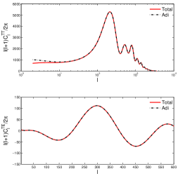
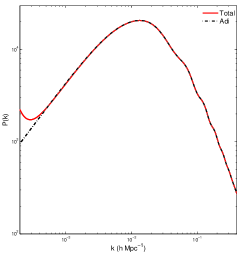
In order to show the effects of the isocurvature perturbations on CMB and LSS observations, we plot in Fig.1 the TT and TE power spectra of CMB and in Fig.2 the matter power spectrum in the case of fully anti-correlation, $\cos\Delta=-1$. In the computations, the fiducial cosmological parameters are chosen as $w_{0}=-1.148$, $w_{a}=1.01$, $c_{se}^{2}=0.01$, $A_{\rm adi}=2.36\times 10^{-9}$, $n_{s}^{\rm adi}=0.95$, $A_{\rm iso}=1.48\times 10^{-8}$, $n_{s}^{\rm iso}=-1.7$, $\omega_{b}=0.02247$, $\omega_{c}=0.1135$, $H_{0}=71.8$km/s/Mpc, where $\omega_{b}\equiv\Omega_{b}h^{2}$ and $\omega_{c}\equiv\Omega_{b}h^{2}$ denote the physical baryon and cold dark matter density parameters, respectively, and $H_{0}=100h$km/s/Mpc is the current Hubble constant. The main effects of isocurvature perturbations of dark energy are on large scales. One can see the suppression in the CMB quadrupole which is realized by the anti-correlation between isocurvature and adiabatic perturbations. However, in the matter power spectrum, there is an increment on large scales with this set of parameters chosen.

Since the effects of isocurvature perturbations appear mainly at large scale, it will be difficult to get a tight constraint on it with current data. This is because we know that in the case of the CMB, the data on large scale is cosmic variance uncertainty dominated, while for LSS the largest scale we can observed today is only about $k=0.02h{\rm Mpc}^{-1}$ sdsslrg7 .

Figure 1: Top Panel: The angular power spectrum of CMB. Bottom Panel: The TE power spectrum of CMB. The red solid lines denote the spectrum obtained including the contribution of anti-correlated adiabatic and isocurvature perturbation, while the black dashed line is obtained by only including the adiabatic contribution.

Figure 2: The matter power spectrum obtained with the cosmological parameters chosen to be the same as in Fig.1. The red line denotes the total power spectrum and the black dash-dotted line is that with only the adiabatic component.

V observational constraints

V.1 Data and Cosmological Parameters

We extended the publicly available MCMC package CosmoMC cosmomc by including dynamical dark energy and its perturbations discussed in this paper. We then performed a global analysis. In the computation of the CMB we have included the WMAP7 temperature and polarization power spectra with the routine for computing the likelihood supplied by the WMAP teamwmap7 . Furthermore, we include small scale temperature anisotropies measured by ACBAR acbar , CBI cbi and Boomerang boomerang . The matter power spectrum measured by observations of luminous red galaxies (LRG) from SDSS sdsslrg7 , and the “Union II” supernovae dataset union2 was also taken into account. Furthermore, we added a prior on the Hubble constant, $H_{0}=74.2\pm 3.6$ km/s/Mpc given by ref.HST as well as a weak Gaussian prior on the baryon density $\omega_{b}=0.022\pm 0.002(1\sigma)$ from Big Bang NucleosynthesisBBN . Simultaneously we also used a cosmic age tophat prior as $10$ Gyr $<t_{0}<20$ Gyr.

In the numerical calculation we considered the most general parameter space

$$\mathcal{\bf P}\equiv\left\{\omega_{b},\omega_{c},\Theta_{s},\tau,w_{0},w_{a},c_{se}^{2},\cos\Delta,n_{s}^{\rm adi},n_{s}^{\rm iso},A_{\rm adi},A_{\rm iso}\right\},$$ (36)

where $\Theta_{s}\equiv 100\frac{r_{s}}{d_{A}}$ is the ratio of the sound horizon to the angular diameter distance at decoupling and $\tau$ characterizes the optical depth to reionization.

V.2 Global Fitting Results

In order to show explicitly the effect of dark energy isocurvature perturbation, we have done two different kinds of calculations: one is with pure adiabatic initial condition by making the three parameters in Eq.(36), i.e. $n_{s}^{\rm iso},A_{\rm iso}$ and $\cos\Delta$ vanish and another is the calculation with the full set of parameters in Eq.(36) including the dark energy isocurvature perturbation (hereafter refer to as “Mixed”). First of all we considered the effect of the isocurvature perturbation on the determination of the dark energy EoS. In Tab.1 we present the numerical values of the dark energy EoS.

	$w_{0}$	$w_{a}$
Adiabatic	$-1.143\pm 0.160$	$0.463\pm 0.605$
Mixed	$-1.132^{+0.164}_{-0.158}$	$0.413^{+0.602}_{-0.610}$

Table 1: Current limits on the dark energy EoS

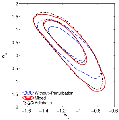
One can see from this table that, given the current observation the isocurvature perturbations makes a change. However the effect is small. As one can see from Fig.1 the cause of the change is the isocurvature mode which suppresses the power spectrum on large scale. Theoretically, to have a sizable suppression, a smaller $w_{e}(a)$ is required in the early universe. This explains why a smaller mean value of $w_{e}(a)$ is obtained in the mixed case given the current data with the suppressed CMB quadrupole. In Fig.3 we plot the two dimensional constraints on the dark energy EoS parameters $w_{0}$, $w_{a}$. To show the importance of dark energy perturbations we also present the results obtained when the DE perturbations switched off incorrectly. We can see from this plot that it brings an error $9\%$ on $w_{0}$ and $52.1\%$ on $w_{a}$.

In Fig.4, we plot the marginalized $1-D$ probability distribution of the parameters related to the initial conditions. The constraints on isocurvature parameters, such as $A_{\rm iso}$, $n_{s}^{\rm iso}$ and $\cos\Delta$ of dark energy are weak. This is understandable, since, as shown in Fig.1 and 2, the isocurvature perturbations of dark energy mainly make contribution at large scale, where the observational data are limited. We note that for the mixed case, the mean value of the adiabatic primordial perturbation amplitude $A_{\rm adi}\sim 2.5\times 10^{-9}$ is slightly larger than in the adiabatic case $A_{\rm adi}\sim 2.4\times 10^{-9}$, while the spectral index is smaller. This indicates that, with respect to adiabatic perturbation, the isocurvature mode has a negative effect on the power spectra on large scale (small $k$), i.e., the mixed mode can suppress the CMB TT angular power spectra at low values of $l$. Moreover, the decrease of $\chi^{2}$, $\Delta\chi^{2}=\chi^{2}_{adi}-\chi^{2}_{mix}\sim 2$ gives a hint that the mixed case is mildly favored by the data.

Figure 3: The constraints on the dark energy EoS parameter $w_{0}$ and $w_{a}$. The red solid lines are for the mixed case and black dash-dotted line for adiabatic case.The blue dashed lines stand for the constraints without dark energy perturbation.

Figure 4: The marginalized 1D probability distribution of the cosmological parameters related to dark energy perturbation.

VI Summary and Discussion

As is well known, cosmological perturbations are crucially important for understanding the CMB anisotropies and structure formation. Up to now the theory of cosmological perturbation is very successful and has been confirmed by the high precision observations and experiments such as WMAP and SDSS. Since the perturbed spacetime is determined by the perturbations of all of the matter components in the universe, it is also important to study the dark energy perturbation. If we naively switch off the dark energy perturbation, the result would be misleading. Moreover, to be general, besides the adiabatic perturbation which is mostly studied in the literature, one should also consider the isocurvature perturbation. Because dark energy couples very weakly to other matter it is not so easy to construct a dark energy model which has purely adiabatic perturbation. Dark energy isocurvature perturbations have important application to lower the quadrupole of the CMB angular power spectrum as needed by the COBE and WMAP observationsquadrupole .

In this paper, we have studied in detail the effects of dark energy isocurvature perturbations. We have included dark energy isocurvature perturbation in the data analysis. By employing a Markov Chain Monte Carlo method, we have performed a global analysis of the determination of the cosmological parameters from current astronomical observational data. We find that isocurvature perturbations decease $\chi^{2}$ by about $2$, and has small effect on other parameters. The current limit on the isocurvature initial condition is weak. We expect that future precision measurements of CMB and LSS on large angular scales, especially the measurements of CMB-LSS cross correlations will lead to a tighter constraint.

References

- (1) A. G. Riess et al. [Supernova Search Team Collaboration], Astron. J. 116, 1009 (1998).
- (2) S. Perlmutter et al. [Supernova Cosmology Project Collaboration], Astrophys. J. 517, 565 (1999).
- (3) H. K. Jassal, J. S. Bagla and T. Padmanabhan, Mon. Not. Roy. Astron. Soc. 405, 2639 (2010). K. M. Wilson, G. Chen and B. Ratra, Mod. Phys. Lett. A 21, 2197 (2006). T. M. Davis et al., Astrophys. J. 666, 716 (2007). S. W. Allen, D. A. Rapetti, R. W. Schmidt, H. Ebeling, G. Morris and A. C. Fabian, Mon. Not. Roy. Astron. Soc. 383, 879 (2008).
- (4) S. Weinberg, Rev. Mod. Phys. 61, 1 (1989).
- (5) P. J. Steinhardt, L. M. Wang and I. Zlatev, Phys. Rev. D 59, 123504 (1999).
- (6) B. Ratra and P. J. E. Peebles, Phys. Rev. D 37, 3406 (1988).
- (7) C. Wetterich, Nucl. Phys. B 302, 668 (1988).
- (8) R. R. Caldwell, R. Dave and P. J. Steinhardt, Phys. Rev. Lett. 80, 1582 (1998).
- (9) R. R. Caldwell, Phys. Lett. B 545, 23 (2002).
- (10) C. Armendariz-Picon, V. F. Mukhanov and P. J. Steinhardt, Phys. Rev. Lett. 85, 4438 (2000).
- (11) B. Feng, X. Wang and Xinmin Zhang, Phys. Lett. B 607, 35 (2005).
- (12) Y. F. Cai, E. N. Saridakis, M. R. Setare and J. Q. Xia, Phys. Rept. 493, 1-60 (2010).
- (13) M. Chevallier and D. Polarski, Int. J. Mod. Phys. D 10, 213 (2001).
- (14) J. Q. Xia, G. B. Zhao, B. Feng, H. Li and Xinmin Zhang, Phys. Rev. D 73, 063521 (2006).
- (15) E. Komatsu et al. [WMAP Collaboration], Astrophys. J. Suppl. 180, 330 (2009).
- (16) C. Yeche, A. Ealet, A. Refregier, C. Tao, A. Tilquin, J. M. Virey and D. Yvon, Astron. Astrophys 448, 831 (2006).
- (17) J. Weller and A. M. Lewis, Mon. Not. Roy. Astron. Soc. 346, 987 (2003).
- (18) R. Bean and O. Dore, Phys. Rev. D 69, 083503 (2004).
- (19) J. Q. Xia, Y. F. Cai, T. T. Qiu, G. B. Zhao and X. Zhang, Int. J. Mod. Phys. D 17 (2008) 1229.
- (20) G. B. Zhao, J. Q. Xia, M. Li, B. Feng and X. Zhang, Phys. Rev. D 72, 123515 (2005).
- (21) P. Mukherjee, A. J. Banday, A. Riazuelo, K. M. Gorski and B. Ratra, Astrophys. J. 598, 767 (2003).
- (22) A. Vikman, Phys. Rev. D 71, 023515 (2005).
- (23) W. Hu, Phys. Rev. D 71, 047301 (2005).
- (24) R. R. Caldwell and M. Doran, Phys. Rev. D 72, 043527 (2005).
- (25) M. Li, B. Feng and Xinmin Zhang, JCAP 0512, 002 (2005).
- (26) X. F. Zhang, H. Li, Y. S. Piao and Xinmin Zhang, Mod. Phys. Lett. A 21, 231 (2006).
- (27) E. A. Lim, I. Sawicki and A. Vikman, JCAP 1005, 012 (2010).
- (28) C. Deffayet, O. Pujolas, I. Sawicki and A. Vikman, JCAP 1010, 026 (2010).
- (29) M. Li, Y. Cai, H. Li, R. Brandenberger and X. Zhang, arXiv:1008.1684 [astro-ph.CO].
- (30) M. Bucher, K. Moodley and N. Turok, Phys. Rev. D 62, 083508 (2000).
- (31) M. Kawasaki, T. Moroi and T. Takahashi, Phys. Rev. D 64 (2001) 083009. M. Kawasaki, T. Moroi, T. Takahashi, Phys. Lett. B533, 294-301 (2002).
- (32) M. Malquarti, A. R. Liddle, Phys. Rev. D66, 123506 (2002).
- (33) T. Moroi and T. Takahashi, Phys. Rev. Lett. 92 (2004) 091301.
- (34) C. Gordon and W. Hu, Phys. Rev. D 70, 083003 (2004).
- (35) H. Li and J. Q. Xia, JCAP 1004, 026 (2010).
- (36) K. Enqvist, H. Kurki-Suonio and J. Valiviita, Phys. Rev. D 62, 103003 (2000).
- (37) D. Langlois, Phys. Rev. D 59, 123512 (1999).
- (38) H. Kurki-Suonio, V. Muhonen and J. Valiviita, Phys. Rev. D 71, 063005 (2005).
- (39) B. A. Reid et al., Mon. Not. Roy. Astron. Soc. 404, 60 (2010).
- (40) A. Lewis and S. Bridle, Phys. Rev. D 66, 103511 (2002).
- (41) E. Komatsu et al., arXiv:1001.4538 [astro-ph.CO].
- (42) C. L. Reichardt, P. A. R. Ade, J. J. Bock et al., Astrophys. J. 694, 1200-1219 (2009).
- (43) A. C. S. Readhead, et al., Astrophys. J. 609 498 (2004).
- (44) C. J. MacTavish, et al., Astrophys. J. 647 799 (2006).
- (45) R. Amanullah et al., Astrophys. J. 716, 712 (2010).
- (46) A. G. Riess et al., Astrophys. J. 699, 539 (2009).
- (47) S. Burles, K. M. Nollett, M. S. Turner, Astrophys. J. 552, L1-L6 (2001).
- (48) C. R. Contaldi, M. Peloso, L. Kofman et al., JCAP 0307, 002 (2003). G. Efstathiou, Mon. Not. Roy. Astron. Soc. 343, L95 (2003). J. -P. Luminet, J. Weeks, A. Riazuelo et al., Nature 425, 593 (2003). R. Bean, O. Dore, Phys. Rev. D69, 083503 (2004). Y. -S. Piao, B. Feng, X. -m. Zhang, Phys. Rev. D69, 103520 (2004). C. J. Copi, D. Huterer, D. J. Schwarz et al., Mon. Not. Roy. Astron. Soc. 367, 79-102 (2006). L. Campanelli, P. Cea, L. Tedesco, Phys. Rev. D76, 063007 (2007). J. Liu, Y. -F. Cai, H. Li, arXiv:1009.3372 [astro-ph.CO].