Gyrokinetic statistical absolute equilibrium and turbulence

Abstract

A paradigm based on the absolute equilibrium of Galerkin-truncated inviscid systems to aid in understanding turbulence [T.-D. Lee, “On some statistical properties of hydrodynamical and magnetohydrodynamical fields,” Q. Appl. Math. 10, 69 (1952)] is taken to study gyrokinetic plasma turbulence: A finite set of Fourier modes of the collisionless gyrokinetic equations are kept and the statistical equilibria are calculated; possible implications for plasma turbulence in various situations are discussed. For the case of two spatial and one velocity dimension, in the calculation with discretization also of velocity $v$ with $N$ grid points (where $N+1$ quantities are conserved, corresponding to an energy invariant and $N$ entropy-related invariants), the negative temperature states, corresponding to the condensation of the generalized energy into the lowest modes, are found. This indicates a generic feature of inverse energy cascade. Comparisons are made with some classical results, such as those of Charney-Hasegawa-Mima in the cold-ion limit. There is a universal shape for statistical equilibrium of gyrokinetics in three spatial and two velocity dimensions with just one conserved quantity. Possible physical relevance to turbulence, such as ITG zonal flows, and to a critical balance hypothesis are also discussed.

I Introduction

Plasma dynamics encompasses a hierarchy of scales with distinct physical processes. At scales much larger than the mean free path and gyroradius, and time scales much larger than the collision time and gyroperiod, the magnetohydrodynamics (MHD) model is good (and is often quite useful over a wider range of collisionality, particularly for phenomena where the parallel kinetic dynamics are not important); while, in the opposite limit of high frequencies and small scales, a complete kinetic description with the Boltzmann or Vlasov equation is necessary. In between, for frequencies well below the ion cyclotron frequency but that may still involve scales comparable to the gyroradius, a detail of the particle helical motion around the field line, the cyclotron angle, may be averaged out, resulting in a reduced system called gyrokinetics.Frieman-Chen ; wwLee83 ; BH07review ; Sch09Review ; Howes06 ; Krommes10 With one dimension (the cyclotron angle) and the fast time scales associated with that dimension excluded, gyrokinetics helps the tractability of turbulent kinetic cascades of plasma turbulence numerically and analytically.

In this contribution, we will present the equilibrium statistical mechanics of the Fourier Galerkin truncated gyrokinetic system and discuss the possible implications for plasma turbulence.

Equilibrium-statistical-mechanics approaches to explore turbulence have long been attempted to identify the flows or to provide some relevant solutions to track the mechanisms of fluid turbulent motions, which have been very illuminating and promising, if not completely successful. UrielBook ; GregSreeniReview One simple but efficient strategy, initiated by Lee,Lee1952 is calculating the Gibbs statistics of the Galerkin-truncated system: The flow of the Euler equation in phase space is incompressible (where the coordinate axes $\sigma_{i}(\textbf{k})$ of this phase space are the real and imaginary parts of the Fourier amplitude of the incompressible velocity field with an upper bound of the wave number $k$), i.e., the dynamics of $\sigma_{i}(\textbf{k})$ satisfies the Liouville theorem, by which an equipartition of energy, which was considered as the conserved quantity, among $\sigma$s was then predicted (c.f. Appendix A for a pedagogical elaboration). There are several reasons that the study of the statistical mechanics of such idealized systems can be of interest.Kraichnan-Montgomery80 ; Taylor97 ; Krommes02 First is that this can give analytic (or semi-analytic) predictions for the equilibrium statistics that can be used as a nonlinear benchmark to test codes. Such nonlinear analytic tests are rare and thus valuable. (This has been useful for fluid codes and, in plasma physics, for particle-in-cell codes,Langdon79 ; Birdsall85 ; KLO86 ; Krommes93 ; Krommes03_MC and could be used for continuum kinetic codes as well.) Second, such analytic spectra can also be useful test cases for analytic theories of turbulence. Equilibrium statistics has been shown to have subtle and deep relevance to statistically nonequilibrium turbulence. It has been used to provide insights into two-dimensional (2D) guiding-center plasma and 2-D vortex fluid models,Taylor71 ; Edwards74 ; Kraichnan-Montgomery80 , and other plasma modelsMontgomery80 ; Gang89 . More recently, it has provided insightsTaylor09 into the unexpected phenomena of spontaneous “spin-up” in bounded 2-D fluid turbulence simulations.Clercx98 ; vanHeijst09 (Interestingly, a current research topic in the fusion field is spontaneous rotation observed in tokamaks.rice:2008 ; solomon:2010 ) The most well-known result from this approach may be the prediction of inverse energy cascade in two dimensional turbulence by Kraichnan, Kraichnan2D67 following which Frisch et al.FrischMHD  calculated the magnetohydrodynamic (MHD) absolute equilibrium and illustrated how the inverse cascade of magnetic helicity may help explain the generation of large-scale magnetic fields in some astrophysical systems. Another example is how the concept of ‘partial thermalization’ has recently been used to understand some observed phenomena such as the ‘bottleneck’ near dissipation scales in Fourier space and the reduction of intermittency, or its scaling, in physical space,FrischPRL08 ; ZhuTaylorCPL2010 which emphasizes the persistence of some aspects of equilibrium statistical mechanics in turbulence, complementing the other side of our knowledge of the persistence of aspects of cascade physics beyond the inertial range (see, e.g., Zhu jzzPRE05 ). Revisiting and further extending such powerful tools to accumulate relevant knowledge and to examine the relevance to definite realities is then important. More recently, this approach has been taken to analyze Hall MHD by Servidio et al.,SMC08 finding that, among others, equipartition of kinetic and magnetic energy predicted by Lee Lee1952 for Alfvénic MHD turbulence no longer holds. Here we will take this paradigm to investigate the gyrokinetic model of plasma turbulence. The nontrivial new feature in our problem is that the integrations over the distributions are functional integrals because of the extra dependence on velocity of the gyrokinetic variable.

More generally, understanding the statistical mechanics of truncated gyrokinetics can help shed light onto the general nature of nonlinear coupling in these equations, and phenomena such as direct or inverse cascades. A better understanding of nonlinear processes in gyrokinetics may also help in the development of more effective sub-grid models for Large-Eddy Simulations, and could improve understanding of the ultimate heating mechanisms as the fluctuations cascade to very small spacial and velocity scales where collisional dissipation occurs.Sch09Review ; Schekochihin08

Related to these sub-grid dissipation issues, the three-dimensional (3D) energy spectrum of thermal fluctuations that we calculate here for a discretized Eulerian gyrokinetic algorithm turns out to be closely related to the noise spectrum calculated earlier for particle-in-cell (Lagrangian) gyrokinetic algorithms.Nevins05

In the two-spatial-and-one-velocity-dimension case, the negative temperature state, leading to the condensation of the generalized energy at the lowest modes, indicates a generic feature of inverse energy cascade. Comparisons are made with some classical results, such as those of Charney-Hasegawa-Mima in the cold-ion limit, though more generally the spectra are modified by finite Larmor radius (FLR) effects which depend on the temperature parameters. The shape of the statistical equilibrium for gyrokinetics in three spatial and two velocity dimensions, where there is just one conserved quantity, has a universal energy spectrum shape, resulting from FLR effects.

In the main body we emphasize the general conceptual ideas with only necessary details for illustration; specific mathematical calculations, physical examples and other interesting digressions are referred to the appendixes for further interests.

II Formulating the problem and calculating the absolute equilibria

To be self-contained, here we very briefly introduce the nonlinear gyrokinetic theoretical framework under which we will be working. We won’t review the complete history of the linear and nonlinear gyrokinetic theories BH07review but will just present the basic ideas and results, borrowing from some of the treatment and notation of Plunk et al.Gabe1 ; Gabe2 There are several published derivations of gyrokinetic equations with varied assumptions and techniques, including recent papers with a tutorial emphasis.Howes06 ; Krommes10 The starting point is the Boltzmann equation for the particle distribution function $f_{s}(\textbf{r},\textbf{v},t)$ for plasma species $s$ located at r moving with velocity v at time $t$:

$$\frac{\partial f_{s}}{\partial t}+{\bf v}\cdot\frac{\partial f_{s}}{\partial\textbf{r}}+\frac{q_{s}}{m_{s}}({\bf E}+\frac{{\bf v}\times{\bf B}}{c})\cdot\frac{\partial f_{s}}{\partial{\bf v}}=C[f_{s}]$$

Here the operator $C[f]$ accounts for the effects of collisions and the particles with mass $m_{s}$ and charge $q_{s}$ are accelerated by the electric (E) and magnetic (B) fields, which are subject to the classical Maxwell equations. The next step is introducing the gyrokinetic ordering (which is fundamentally to focus on fluctuations that are low frequency compared to the fast gyromotion of particles around the magnetic field) and the resulting expansion parameter. A key operation in the resulting equations is the average of any particular quantity $\Psi$ around a ring of gyroradius $\rho$ perpendicular ($\perp$) to the magnetic field direction ($\parallel$) surrounding the gyrocenter R:Note1

$$\langle\Psi\rangle_{\textbf{R}}=\frac{\int\Psi(\textbf{r})\delta(\textbf{r}_{\parallel}-\textbf{R}_{\parallel})\delta[|\textbf{r}_{\perp}-\textbf{R}_{\perp}|-\rho(\textbf{R})]d^{3}\textbf{r}}{2\pi\rho(\textbf{R})}.$$ (1)

Using a Fourier representation $\Psi(\textbf{r})=\sum_{k}\exp(-i\textbf{k}\cdot\textbf{r})\hat{\Psi}_{\textbf{k}}$, and considering a straight magnetic field for simplicity here, this becomes $\langle\Psi\rangle_{\textbf{R}}=\sum_{\textbf{k}}\exp(-i\textbf{k}\cdot\textbf{R})J_{0}(k_{\mbox{$\scriptscriptstyle\perp$}}\rho)\hat{\Psi}_{\textbf{k}}$, where $J_{0}$ is a Bessel function.

Writing $\textbf{v}=\textbf{v}_{\perp}+v_{\parallel}\hat{\textbf{z}}$ and $f=F_{01}+h+h.o.t.$ (and suppressing the species subscript $s$ for now), with $h.o.t.$ representing “higher order terms,” the resulting gyrokinetic equations for the case of slab geometry with a homogeneous plasma in a straight equilibrium magnetic field $\textbf{B}_{0}=B_{0}\hat{\textbf{z}}$) is

$$\frac{\partial h}{\partial t}+v_{\parallel}\hat{\textbf{z}}\cdot\frac{\partial h}{\partial\textbf{R}}+\frac{c}{B_{0}}\left(\hat{\textbf{z}}\times\frac{\partial\langle\chi\rangle_{\textbf{R}}}{\partial\textbf{R}}\right)\cdot\frac{\partial h}{\partial\textbf{R}}={q}\frac{\partial\langle\chi\rangle_{\textbf{R}}}{\partial t}\frac{F_{0}}{T_{0}},$$

complemented with the similar ordering-gyroaveraging treatment of the Maxwell equations for the electrostatic potential $\varphi$ and the perturbed vector potential A which compose the gyrokinetic potential $\chi=\varphi-\textbf{v}\cdot\textbf{A}/c$. Here the collisional term is omitted. The zeroth and first order term $F_{01}$ is in general taken to be the equilibrium Maxwell distribution ($F_{0}$) multiplied by a Boltzmann factor, $\exp(-q\varphi/T_{0})\approx 1-q\varphi/T_{0}$. In what follows below, as in Plunk et al.,Gabe1 ; Gabe2 we will work with the gyroaveraged, perturbed, guiding center distribution function $g=h-F_{0}q\langle\varphi\rangle_{R}/T_{0}$, instead of with the non-adiabatic component $h$, and for simplicity we will focus on the case of electrostatic fluctuations (neglecting magnetic fluctuations, $\textbf{A}=0$) with one particle species governed by the gyrokinetic equation and the other species having a Boltzmann response of some form (discussed below).

To make it easier to compare with other codes and theories that use a variety of normalizations, and in particular to make it easier to take the cold-ion limit in 2-D to compare with the Hasegawa-Mima equations, we will use a generalized normalization for space and time scales based on a reference temperature $T_{r}$, a reference sound speed $c_{r}=\sqrt{T_{r}/m}$, and a reference gyroradius $\rho_{r}=c_{r}/\Omega_{c}$, (here the mass $m$ and Larmor (cyclotron) frequency $\Omega_{c}=qB/mc$ are for the species that is governed by the gyrokinetic equation), but still scale $v_{\mbox{$\scriptscriptstyle\|$}}$ and the velocity dependence of $F_{0}$ and $g$ to $\mbox{$v_{\mbox{\scriptsize{th}}}$}=\sqrt{T_{0}/m}$, where $T_{0}$ is the temperature of the gyrokinetic species. More specifically, we use the following normalizations and definitions, with physical (dimensional) variables having subscript ‘p’:

$t=t_{\mbox{\scriptsize{p}}}c_{r}/L$	$x=x_{\mbox{\scriptsize{p}}}/\rho_{r}$	$y=y_{\mbox{\scriptsize{p}}}/\rho_{r}$	$z=z_{\mbox{\scriptsize{p}}}/L$
$v_{{\mbox{$\scriptscriptstyle\perp$}},{\mbox{$\scriptscriptstyle\|$}}}=\frac{v_{{\mbox{$\scriptscriptstyle\perp$}},{\mbox{$\scriptscriptstyle\|$}},\mbox{\scriptsize{p}}}}{\mbox{$v_{\mbox{\scriptsize{th}}}$}}$	$\mbox{$\varphi$}=\mbox{$\varphi$}_{\mbox{\scriptsize{p}}}\frac{qL}{T_{r}\rho_{r}}$	$h=h_{\mbox{\scriptsize{p}}}\frac{\mbox{$v_{\mbox{\scriptsize{th}}}$}^{3}L}{n_{0}\rho_{r}}$	$F_{0}=\frac{F_{0\mbox{\scriptsize{p}}}\mbox{$v_{\mbox{\scriptsize{th}}}$}^{3}}{n_{0}}$

The equilibrium density and temperature of the gyrokinetic species of interest are $n_{0}$ and $T_{0}$; the thermal velocity is $\mbox{$v_{\mbox{\scriptsize{th}}}$}=\sqrt{T_{0}/m}$; $L$ is the reference macroscopic scale length (i.e., system size), satisfying $\rho/L\ll 1$ for consistency with gyrokinetic ordering.

In these normalized units, the Maxwellian background distribution function is given by $F_{0}=\exp(-(v_{\mbox{$\scriptscriptstyle\perp$}}^{2}+v_{\mbox{$\scriptscriptstyle\|$}}^{2})/2)/(2\pi)^{3/2}$, and the gyrokinetic equation for the gyroaveraged, perturbed, guiding center density $g(\textbf{R},v_{\mbox{$\scriptscriptstyle\|$}},v_{\mbox{$\scriptscriptstyle\perp$}},t)$ is given by

$$\frac{\partial g}{\partial t}+\rho_{0}v_{\parallel}\frac{\partial g}{\partial z}+\left(\hat{\textbf{z}}\times\frac{\partial\langle\mbox{$\varphi$}\rangle_{\textbf{R}}}{\partial\textbf{R}}\right)\cdot\frac{\partial g}{\partial\textbf{R}}=-\frac{v_{\mbox{$\scriptscriptstyle\|$}}}{\rho_{0}}\frac{\partial\langle\mbox{$\varphi$}\rangle_{\textbf{R}}}{\partial z}F_{0},$$

where $\rho_{0}=\rho_{th}/\rho_{r}=\mbox{$v_{\mbox{\scriptsize{th}}}$}/c_{r}=\sqrt{T_{0}/T_{r}}$ is the thermal gyroradius $\rho_{th}$ of the gyrokinetic species normalized to the reference gyroradius $\rho_{r}$. (Our normalization reduces to that used in Plunk et al.Gabe1 ; Gabe2  if we choose $T_{r}=T_{0}$ so $\rho_{0}=1$, which in fact we will do in the 3-D case.)

The gyrokinetic equation expresses how the guiding centers evolve in time due to parallel motion along the magnetic field, the gyro-averaged $\textbf{E}\times\textbf{B}$ drift across the magnetic field (this is the nonlinear term), and parallel electric field acceleration. (Note that the slow $\textbf{E}\times\textbf{B}$ drift of the guiding center location R is different than the rapid gyration velocity $v_{\mbox{$\scriptscriptstyle\perp$}}$ of a particle around its guiding center.)

This equation is closed by using the gyrokinetic quasi-neutrality equation to determine the electrostatic potential, which in Fourier space with these normalized units is given by

$$\hat{\varphi}(\textbf{k},t) = \frac{\beta(\textbf{k})}{2\pi}\int d^{3}vJ_{0}(k_{\mbox{$\scriptscriptstyle\perp$}}\rho_{0}v_{\mbox{$\scriptscriptstyle\perp$}})\hat{g}(\textbf{k},v_{\mbox{$\scriptscriptstyle\|$}},v_{\mbox{$\scriptscriptstyle\perp$}},t)$$

$$= \beta(\textbf{k})\!\int_{-\infty}^{\infty}\!\!dv_{\mbox{$\scriptscriptstyle\|$}}\int_{0}^{\infty}\!\!dv_{\mbox{$\scriptscriptstyle\perp$}}v_{\mbox{$\scriptscriptstyle\perp$}}J_{0}(k_{\mbox{$\scriptscriptstyle\perp$}}\rho_{0}v_{\mbox{$\scriptscriptstyle\perp$}})\hat{g}(\textbf{k},v_{\mbox{$\scriptscriptstyle\|$}},v_{\mbox{$\scriptscriptstyle\perp$}},t),$$

where

$$\beta(\textbf{k})=\frac{2\pi}{\tau({\bf k})+\frac{T_{r}}{T_{0}}(1-\hat{\Gamma}(k_{\mbox{$\scriptscriptstyle\perp$}}^{2}\rho_{0}^{2}))},$$ (4)

$\hat{\Gamma}(k^{2})=I_{0}(k^{2})e^{-k^{2}}$ is an exponentially-scaled modified Bessel function, $I_{0}(k^{2})=J_{0}(ik^{2})$, and $\tau({\bf k})$ represents the shielding by the species that is treated as having a Boltzmann response of some form, the choice of which depends on physical situation. If we are treating the ions gyrokinetically (such as for ion-scale drift waves or Ion Temperature Gradient-driven turbulence) and using an adiabatic approximation for electrons because of their fast parallel motion relative to a typical frequency, $k_{\mbox{$\scriptscriptstyle\|$}}v_{te}\gg\omega$ (except for modes with $k_{\mbox{$\scriptscriptstyle\|$}}=0$), then $\tau(\textbf{k})=(T_{r}/T_{e})(1-\delta_{k_{\mbox{$\scriptscriptstyle\|$}}})$, where $T_{e}$ is the electron temperature and the discrete Kronecker $\delta$ function ensures that the electrons do not respond to zonal modes with $k_{\mbox{$\scriptscriptstyle\|$}}=E_{\mbox{$\scriptscriptstyle\|$}}=0$. If we are treating electrons gyrokinetically (such as for small electron scale Electron Temperature Gradient-driven turbulence) with an adiabatic approximation for ions because $k_{\perp}v_{ti}\gg\omega$ (the $k_{\perp}=0$ mode is not driven by any nonlinearities in a periodic domain), then $\tau=T_{r}/T_{i}$.

Finally, one can also consider a no-response model, $\tau=0$, which in the 2-D cold-ion limit $T_{0}\rightarrow 0$ leads to $\beta\rightarrow 2\pi/k_{\mbox{$\scriptscriptstyle\perp$}}^{2}$, $J_{0}\rightarrow 1$, and the gyrokinetic equation reduces to 2-D hydrodynamics.

The above difference in zonal flow dynamics for ion vs. electron scale fluctuations is responsible for a large enhancement in zonal flows for ion-scale turbulence, so that zonal flows play a key role in the saturation dynamics of ITG turbulenceHammett93 ; Dorland93 ; Cohen93 and leads to the Dimits nonlinear shift in the critical gradient.Dimits96 ; Dimits00 It is also responsible for a significant reduction in the effect of zonal flows for electron-scale turbulence, so that they can get to larger amplitude than one would at first expect from scaling from ion-scale turbulence.Jenko2000 ; Dorland2000

II.1 2D Gyrokinetic absolute equilibria

For a plasma in a two dimensional ($\partial/\partial z=0$) cyclic box, the collisionless gyrokinetic equation in wavenumber space reads

$$\partial_{t}\hat{g}(\textbf{k},v)=\hat{\textbf{z}}\times\sum_{\textbf{p}+\textbf{q}=\textbf{k}}\textbf{p}J_{0}(p\rho_{0}v)\hat{\varphi}(\textbf{p})\cdot\textbf{q}\,\hat{g}(\textbf{q},v)$$ (5)

with the potential $\varphi$ determined by the quasi-neutrality condition

$$\hat{\varphi}(\textbf{k})=\beta(\textbf{k})\int vdvJ_{0}(k\rho_{0}v)\hat{g}(\textbf{k},v),$$ (6)

where the subscript on $v_{\mbox{$\scriptscriptstyle\perp$}}$ has been dropped and the parallel velocity $v_{\mbox{$\scriptscriptstyle\|$}}$ has been integrated out of the problem.

The only known rugged (still conserved after mode truncation) invariants are the “energy” $\mathrm{E}=(1/2V)\int d^{2}\textbf{r}[(\tau+(T_{r}/T_{0}))\varphi^{2}-(T_{r}/T_{0})\varphi\Gamma\varphi]$, and a parameterized set of invariants related to the “perturbed-entropy” $\mathrm{G}(v)=(1/2V)\int d^{2}\textbf{R}g^{2}$ (in these equations, $V$ is the volume (area) of the integration domain and $\Gamma$ is a convolution operator in real space given by the Fourier transform of $\hat{\Gamma}$). (See Refs.(Gabe1, ; Gabe2, ; Sch09Review, ) and references therein for a discussion of these conserved quantities and their interpretation.) In Fourier space these become $\mathrm{E}=$ $\pi\sum_{\textbf{k}}|\mbox{$\varphi$}_{k}|^{2}/\beta({\textbf{k}})$ and $\mathrm{G}(v)=$ $\sum_{\textbf{k}}|g({\bf k},v)|^{2}/2$. As promised in the introductory discussion, following Lee,Lee1952 in what follows we will keep summations over only a finite subset $\mathbb{K}$ of all possible wavenumbers k—the Fourier Galerkin truncation. Note2 The Fourier modes in the lower half plane are determined by the reality condition, $g(-\mathbf{k},v)=g^{*}(\mathbf{k},v)$, so the state of a system can be uniquely specified by the values of the real and imaginary parts of the Fourier coefficients $g(\mathbf{k},v)$ for wavenumbers in the upper half plane. We will thus consider a further subset $\mathbb{K}^{+}$, defined as the modes in $\mathbb{K}$ in the upper half plane, which satisfy $k_{y}\geq 0$ if $k_{x}>0$, or $k_{y}>0$ if $k_{x}\leq 0$ (see also Krommes and RathKrommes03_MC ). All spectral sums will be expressed in terms of the finite set of independent modes in $\mathbb{K}^{+}$, and we denote this summation by $\tilde{\sum}_{\bf k}$.

We can discretize Eq. (6) into

$$\tilde{\hat{\varphi}}(\textbf{k})=\beta(\textbf{k})\sum_{i=1}^{N}w_{i}(k)\hat{g}(\textbf{k},v_{i}),$$ (7)

where $w_{i}(k)=m_{i}v_{i}J_{0}(k\rho_{0}v_{i})$, and $m_{i}$ is the weight of velocity grid point $v_{i}$. This discrete form can correspond to the case that $\hat{g}(\textbf{k},v)$ is uniform on the lattice around node $i$; in general, it is used as a numerical approximation for the arbitrary distribution over $v$ as applied in the present continuum codes.Note3 For a simple midpoint integration rule on a grid that extends up to some maximum velocity $v_{max}=v_{N}$, the weight is given by the grid spacing, $m_{i}=\Delta v_{i}$. (More general integration algorithms can also be represented in this form.Note4 ) With this velocity discretization, there are now $N+1$ conserved quantities, given by the energy $\tilde{E}=\tilde{\sum}_{\bf k}2\pi\beta({\bf k})\sum_{i,j}^{N}w_{i}\hat{g}^{*}(\textbf{k},v_{i})w_{j}\hat{g}(\textbf{k},v_{j})$ and the entropy-related quantities $\tilde{G}_{i}=\tilde{\sum}_{\bf k}|\hat{g}(\textbf{k},v_{i})|^{2}$.

So, with the common belief of the applicability of Gibbsian statistical mechanics or Jaynes’ Jaynes57I ; Jaynes57II idea of “statistical mechanics as a form of statistical inference", we have the distribution function $\sim\exp\{-\tilde{\mathcal{S}}\}$, where $\tilde{\mathcal{S}}$ is a linear combination of conserved quantities, which will be written as

$$\tilde{\mathcal{S}}= \sum_{i=1}^{N}\alpha_{i}\tilde{G}_{i}+\alpha_{0}\tilde{E}.$$ (8)

Here, the $\alpha_{i}$ are the “(inverse) temperature parameters” introduced as Lagrangian multipliers to form the constant of the motion. The Gibbs measure can be shown to be conserved by the flow as a generalized Liouville theorem, the incompressibility of the flow of the phase points in the hyperplane spanned by the real and imaginary parts of the Fourier modes.Lee1952 Note that, importantly, conservation laws and the Liouville theorem are inherited, which, with some more assumptions (such as ergodicity) makes the discrete system possible to produce a Gibbs ensemble. A pedagogical illustration on the Gibbs canonical distribution for this system can be found in Appendix A.

As this is a multivariate Gaussian distribution, one can numerically invert the matrix of the quadratic form $\mathcal{S}=\sum_{i,j}[\delta_{ij}\alpha_{i}+\alpha_{0}2\pi\beta(\textbf{k})w_{i}(k)w_{j}(k)]\hat{g}(\textbf{k},v_{i})\hat{g}^{\ast}(\textbf{k},v_{j})$, but, actually, using the Sherman-Morrison formula (see Appendix B), one can write down the $N\times N$ covariances

$$c_{i,j}(\textbf{k}) = \langle g^{*}(\textbf{k},v_{i})g(\textbf{k},v_{j})\rangle/2$$ (9)

$$= \frac{\delta_{i,j}}{2\alpha_{i}}-\frac{\alpha_{0}\pi\beta(\textbf{k})w_{i}\alpha_{i}^{-1}w_{j}\alpha_{j}^{-1}}{1+\alpha_{0}2\pi\beta(\textbf{k})\sum_{l}w_{l}^{2}\alpha_{l}^{-1}}.$$

The spectral energy density $D(\textbf{k})$ then can be calculated as follows:

$$D(\textbf{k}) =\frac{\pi}{\beta(\textbf{k})}\langle\left|\hat{\varphi}(\textbf{k})\right|^{2}\rangle=2\pi\beta(\textbf{k})\sum_{i,j}w_{i}w_{j}c_{ij}$$ (10)

$$=\frac{\pi\beta(\textbf{k})\sum_{l}w_{l}^{2}(\alpha_{l})^{-1}}{1+\alpha_{0}2\pi\beta(\textbf{k})\sum_{l}w_{l}^{2}\alpha_{l}^{-1}}.$$

The isotropic energy spectrum then is $E(k)\sim kD(\textbf{k})$. The spectral density of the perturbed entropy $\mathrm{G}_{i}$ is

$$\mathrm{G}_{i}(\textbf{k}) = \frac{1}{2}\langle\left|\hat{g}(\textbf{k},v_{i})\right|^{2}\rangle=c_{i,i}(\textbf{k})$$ (11)

$$= \frac{1}{2\alpha_{i}}\left[1-\frac{\alpha_{0}2\pi\beta(\textbf{k})w_{i}^{2}\alpha_{i}^{-1}}{1+\alpha_{0}2\pi\beta(\textbf{k})\sum_{l}w_{l}^{2}\alpha_{l}^{-1}}\right],$$

which expresses the nearly equipartition on Fourier modes when the second term in the brackets has negligible contribution.Zhu20103 (Note that $D({\bf k})$ and $G_{i}({\bf k})$ depend on wavenumber not only through $\beta({\bf k})$ but also through $w_{i}=w_{i}(k)$.)

The temperature parameters are determined by the values of the invariants $\tilde{G}_{i}$ and $\tilde{E}$. Note that these give the invariants as nonlinear functions of the temperature parameters $\alpha_{0}$ and $\alpha_{i}$, so this requires numerical solution or further analytic approximations to invert.

Discussion concerning 2+1D gyrokinetic spectra

To gain insight into the behavior of these spectra, we will explore them in various simplifying limits, such as the small and large-$k$ limits and the cold-ion Hasegawa-Mima limit. We will also plot example spectra for particular values of the $\alpha_{0}$ and $\alpha_{i}$ parameters.

The gyroaveraging by plasma particles through Eq. (1) (finite Larmor radius effects) introduces several special functions whose asymptotic behaviors help shape the energy spectrum. For convenience, let’s write here the asymptotic recipes for these special functions:

$k\to 0,$	$\!J_{0}(k\rho_{0}v_{i})\approx 1-k^{2}\rho_{0}^{2}v_{i}^{2}/4,$	$\,\,\hat{\Gamma}(k^{2}\rho_{0}^{2})\approx 1-k^{2}\rho_{0}^{2}$
$k\to\infty,$	$J_{0}^{2}(k\rho_{0}v_{i})\sim\frac{2\cos^{2}(kv_{i}-\pi/2)}{(\pi kv_{i})},$	$\hat{\Gamma}(k^{2}\rho_{0}^{2})\sim\frac{1}{\sqrt{2\pi}k\rho_{0}}$

The simplest limit to consider first is $\rho_{0}=\sqrt{T_{0}/T_{r}}\rightarrow 0$, i.e., the cold-ion limit considered by Hasegawa and Mima in their study of drift-wave turbulence HMpof78 (see Appendix C for more details). The Hasegawa-Mima equation coincides with the Charney equation for geophysical flowsCharney71 formulated earlier, so it is also called the Charney-Hasegawa-Mima (CHM) equation.

In this limit, $J_{0}(k\rho_{0}v)\rightarrow 1$, and $w_{i}(k)=m_{i}v_{i}J_{0}(k\rho_{0}v)\rightarrow m_{i}v_{i}$ so the factor of $\sum_{l}w_{l}^{2}(k)/\alpha_{l}$ in Eq. (10) becomes independent of $k$ and can just be taken as a constant, which we will define as $1/(2\pi^{2}\bar{\alpha})$. In the expression for $\beta({\bf k})$ in Eq. (4), we use $\hat{\Gamma}(k^{2}\rho_{0}^{2})\rightarrow 1-k^{2}\rho_{0}^{2}$ and find $\beta({\bf k})\rightarrow 2\pi/(\tau+k^{2})$. For comparison with Hasegawa and Mima, we set the reference temperature to the electron temperature, $T_{r}=T_{e}$, (the electrons are the adiabatic species for ion-scale drift waves) and neglect the $\delta_{k{\mbox{$\scriptscriptstyle\|$}}}$ factor and associated zonal flow effects Note5 in the expression for $\tau$ so that $\tau=1$. Note that our normalized $k=k_{\mbox{$\scriptscriptstyle\perp$}}=k_{{\mbox{$\scriptscriptstyle\perp$}},p}\rho_{s}$, where $k_{{\mbox{$\scriptscriptstyle\perp$}},p}$ is the physical perpendicular wavenumber, and $\rho_{s}=\sqrt{T_{e}/m_{i}}/\Omega_{ci}$ is the ion sound radius. (Alternatively, one can consider these as equations for electron-scale turbulence where the role of ions and electrons is reversed: the ions are adiabatic and a cold electron limit is used, in which case the normalizing length is an “electron sound radius”, $\rho_{se}=\sqrt{T_{i}/m_{e}}/\Omega_{ce}$.)

The result is that the isotropic energy spectrum given by Eq. (10) reduces in the cold ion limit to

$$E(k)\propto kD(k)\propto\frac{k}{\bar{\alpha}(1+k^{2})+2\alpha_{0}},$$ (12)

where $\bar{\alpha}$ and $\alpha_{0}$ are coefficients that are determined by the values of the invariants $E$ and $G_{i}$. Note that this is of the same form of a 2-parameter family of spectra as in Charney-Hasegawa-Mima (CHM) or 2-D Euler absolute equilibrium, $E(k)\propto k/(\alpha_{CHM}+\beta_{CHM}k^{2})$ (Appendix C).

A remarkable feature of this type of spectrum is that if $\alpha_{CHM}$ or $\beta_{CHM}$ are negative, corresponding to a negative temperature, then the denominator has the opportunity of tending to zero leading to the energy condensation at the lowest or highest wave numbers. Energy condensation to the lowest modes (one example is shown in Fig. 1) would indicate an inverse cascade of energy following the argument of Kraichnan for the 2D Euler equation Kraichnan2D67 (see also Hasegawa and Mima HMpof78 , and, Fyfe and Montgomery.FMpof79 ) It then seems that the inverse cascade of energy in 2D gyrokinetics could be quite a generic feature: Recent relevant theoretical arguments and numerical simulation results Sch09Review ; Gabe2 ; TomoPRL09 are consistent with this.

Instead of the cold-ion limit, we now consider the more general case of warm ions (for ion-scale turbulence, or warm electrons for electron-scale turbulence), and for simplicity let us take $T_{e}=T_{i}=T_{r}$ (so that $\rho_{0}=1$) and neglect zonal flow effects (so that $\tau=1$). In the limit $k\gg 1$, we have $\beta(\textbf{k})\rightarrow\pi$, and the magnitude of $w_{i}(k)^{2}\propto J_{0}^{2}(kv_{i})$ will be bounded by $C/(kv_{i})$ for some constant $C$. Assuming positive $\alpha_{i}$ for $i>0$, we find that the denominator in Eq. (10) approaches 1 for large $k$, so $D(k)\sim 1/k$ and $E(k)\sim kD(k)\sim k^{0}$. This could give a larger tail for gyrokinetics than for CHM, which has $E_{CHM}(k)\sim 1/k$ (for $\beta_{CHM}>0$). In this same $k\gg 1$ limit, Eq. (11) simplifies to $G_{i}({\bf k})=1/(2\alpha_{i})$, which corresponds to equipartition of the generalized entropy. We plot the spectra over the reachable wave number regime with given temperatures just to sketch the physical picture without even bothering to accurately calculate the realizable wave number bounds but only with estimations sufficient to directly illustrate the problem. (Another way to think about the problem and do the corresponding plots is to take the bounds of wavenumbers to be prescribed and then realizable temperature parameters are determined accordingly. Detailed computations and illustrations of more example spectra with possible physical discussions are given in Appendix D for those who are interested.) Actually, much is already known from the knowledge of absolute equilibria of 2D Euler Kraichnan2D67 and Hasegawa-Mima HMpof78 , though it may still be helpful to give some general physical picture, especially the finite Larmor radius effects, with some example spectra as shown in Fig.1: The $\alpha_{i}$ for $i>0$ were set by $\alpha_{i}^{-1}=10^{-3}\exp(-v_{i}^{2}/2)$. We take $N=40$ with $v_{i}$ homogeneously collocated between $0$ and $V=3$, and, $\mathbb{K}=\{\textbf{k}|1\leqslant k_{x,y}\leqslant 150\}$ for positive temperatures cases while $\mathbb{K}=\{\textbf{k}|4\leqslant k_{x,y}\leqslant 150\}$ for a negative temperature case. Some details, including the values of $m_{i}$ ($=1$ here), are not important, and reasonable changing of them (as a re-normalization of the variables) won’t affect our results. Here, as $E(k)\sim kD(\textbf{k})$, the low-$k$ equipartition range have $E(k)\sim k$ and $E(k)\sim k^{0}$ for large $k$, both of which can be easily checked with the asymptotic recipe of the special functions given in the beginning of this subsection. The transition in between represents the FLR effects, the details of which also depend on the details of the temperature parameters. Other temperature parameter values may change the $k$ ranges where such asymptotic behaviors can be realized; or, if the truncation wave numbers in the computations $k_{min}$ and $k_{max}$ (which may be relevant to some characteristic, such as the collisional, scales in real physical systems) were not chosen properly, we would not be able to reach such asymptotic behaviors.

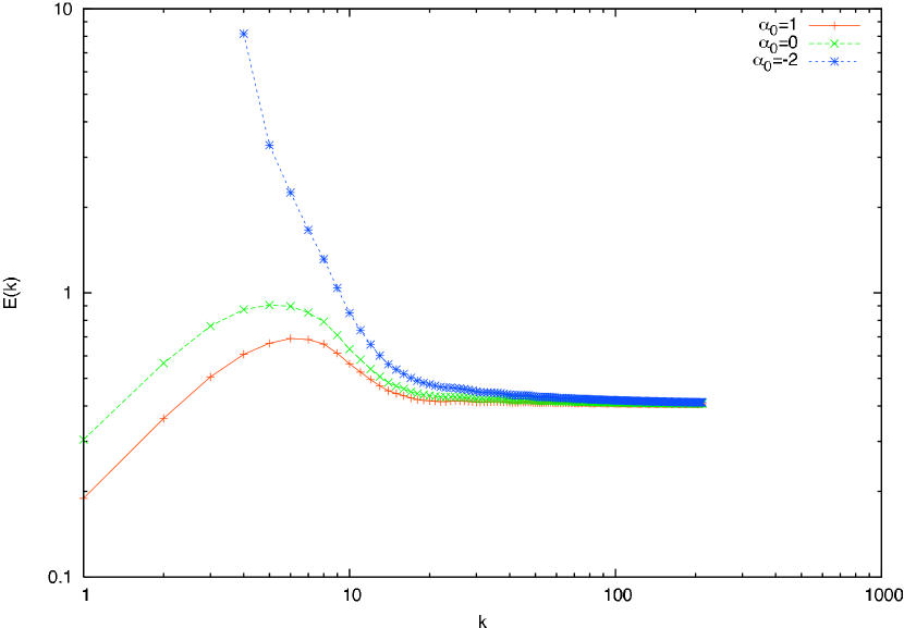
Figure 1: (Color online) Example spectra for various values of $\alpha_{0}$, with $\alpha_{i}=10^{3}\exp\{v_{i}^{2}/2\}$ for $i>0$, and $\rho_{0}=10^{-1}$, $\tau=1$. Negative $\alpha_{0}$ state can occur that correspond to condensation of most of the energy into the longest wavelength modes.

A negative value of $\alpha_{0}$ corresponds not only to an enhancement of energy at larger spatial scales (low $k$) but also to an enhancement of fluctuations at larger velocity scales, as given by Eq. (9). If $\alpha_{0}=0$, then this equation indicates that different velocity grid points $i\not=j$ are uncorrelated, while making $\alpha_{0}$ more negative will increase the correlation length in the velocity, particularly at low $k$. If collisions are included, they will cause dissipation at both small velocity scales and small spatial scales (through FLR effects corresponding to classical diffusion),Abel08 so the inverse cascade found here in 2D will tend to reduce both forms of dissipation.

We end up this sub-section by remarking that, since the CHM limit absolute equilibrium statistics has already been verified by numerical experiment,FMpof79 our theoretical calculation for gyrokinetic is then also, to some degree, endorsed.

II.2 3+2D Gyrokinetic absolute equilibria

The mathematical treatment for the calculation of Galerkin truncation absolute equilibrium is basically the same for 3+2D and 2+1D cases. However, some brief remarks about the system and the conserved quantity, followed by some technical details in the calculation are still necessary.

In the full gyrokinetic equation with three spatial and two velocity dimensions, notice that two linear terms, from parallel motion along the magnetic field and from the parallel electric field acceleration, are simply added to the equation for the $(2+1)$-D case, without changing anything about the nonlinear term. While the gyroaveraged E cross B drift conserves $E$ and $G$ separately, the parallel motion makes them talk to each other and combines them into another conserved quantity, the generalized energy $W=E+W_{g0}$ (see Refs.(Gabe2, ; Sch09Review, ; Schekochihin08, ; Krommes94, ) and references therein for further discussions of this quantity):

$$W=\int\frac{d^{3}\mathbf{r}}{2V}[(1+\tau)\varphi^{2}-\varphi\Gamma\varphi]+\int d^{3}v\int\frac{d^{3}\mathbf{R}}{2V}\frac{g^{2}}{F_{0}}.$$ (13)

(For simplicity in all of our 3+2D work, we will set the reference temperature $T_{r}$ used in normalizations to the temperature of the kinetic species $T_{0}$, so $\rho_{0}=1$.) The Fourier Galerkin truncated form of the generalized energy is

$$S=2\tilde{\sum}_{\bf k}\Bigg{\{}\frac{\pi}{\beta(\textbf{k})}|\hat{\varphi}(\mathbf{k})|^{2}+\pi\int\!\!\!\!\!\int v_{\perp}dv_{\perp}dv_{\parallel}\frac{|\hat{g}(\mathbf{k},{\bf v})|^{2}}{F_{0}}\Bigg{\}}.$$

We will discretize velocity space in a way that makes it easy to reduce the previous 2D spatial + 1D velocity results to the 3D spatial + 2D velocity results here. Specifically, we will discretize velocity integrals as

$$\int d^{3}vg({\bf v}) = 2\pi\int_{0}^{\infty}dv_{\mbox{$\scriptscriptstyle\perp$}}\int_{-\infty}^{\infty}dv_{\mbox{$\scriptscriptstyle\|$}}v_{\mbox{$\scriptscriptstyle\perp$}}g(v_{\mbox{$\scriptscriptstyle\|$}},v_{\mbox{$\scriptscriptstyle\perp$}})$$ (14)

$$\approx 2\pi\sum_{i}^{N}m_{i}v_{{\mbox{$\scriptscriptstyle\perp$}},i}g({\bf v}_{i}),$$

where $i$ now indexes over all points ${\bf v}_{i}=(v_{{\mbox{$\scriptscriptstyle\perp$}}i},v_{{\mbox{$\scriptscriptstyle\|$}}i})$ in the 2D velocity space grid. For a logically rectangular mesh in $(v_{\mbox{$\scriptscriptstyle\perp$}},v_{\mbox{$\scriptscriptstyle\|$}})$ there would be a total of $N=N_{v_{\mbox{$\scriptscriptstyle\perp$}}}N_{v_{\mbox{$\scriptscriptstyle\|$}}}$ grid points, with $N_{v_{\mbox{$\scriptscriptstyle\perp$}}}$ points in the perpendicular velocity direction and $N_{v_{\mbox{$\scriptscriptstyle\|$}}}$ in the parallel velocity direction. (As in the 1D velocity case, for a simple midpoint integration algorithm, $m_{i}$ is the weight of the $i$’th velocity cell, $m_{i}=\Delta v_{{\mbox{$\scriptscriptstyle\perp$}},i}\Delta v_{{\mbox{$\scriptscriptstyle\|$}},i}$, while more generally the weights $m_{i}$ and grid point locations $(v_{{\mbox{$\scriptscriptstyle\perp$}},i},v_{{\mbox{$\scriptscriptstyle\|$}},i})$ can be chosen to give high-order Gaussian quadrature.) The 2D velocity generalization of Eq. (7), the discretized quasineutrality equation to determine the potential, now reads $\hat{\mbox{$\varphi$}}(\textbf{k})=\beta(\textbf{k})\sum_{i}w_{i}(k_{\mbox{$\scriptscriptstyle\perp$}})\hat{g}(\textbf{k},\textbf{v}_{i})$, where $w_{i}(k_{\mbox{$\scriptscriptstyle\perp$}})=m_{i}v_{{\mbox{$\scriptscriptstyle\perp$}},i}J_{0}(k_{\mbox{$\scriptscriptstyle\perp$}}v_{{\mbox{$\scriptscriptstyle\perp$}},i})$.

We then can calculate the absolute equilibria following the same procedure as in the 2D case, but now only one inverse temperature parameter $\gamma$ shows up in the canonical distribution $\sim\exp\{-\gamma S\}$. Using the above velocity discretization for $\tilde{\cal S}=\gamma S=\gamma(E+W_{g0})$ gives

$$\tilde{\mathcal{S}} = \gamma\tilde{\sum}_{\bf k}2\pi\beta(\textbf{k})\Sigma_{i,j}w_{i}\hat{g}^{*}(\textbf{k},{\bf v}_{i})w_{j}\hat{g}(\textbf{k},{\bf v}_{j})$$

$$+\gamma\Sigma_{i=1}^{N}2\pi m_{i}v_{{\mbox{$\scriptscriptstyle\perp$}},i}\tilde{\sum}_{\bf k}|\hat{g}(\textbf{k},{\bf v}_{i})|^{2}/F_{0}(v_{i})$$

We note from this that a negative temperature is not realizable any more. Comparing this expression for the 3D $\tilde{\cal S}$ with the 2D result in Eq. (17), we see that they become identical if we make the substitutions $\alpha_{0}=\gamma$ and $\alpha_{i}=2\pi\gamma m_{i}v_{{\mbox{$\scriptscriptstyle\perp$}},i}/F_{0}(\textbf{v}_{i})$. All of the 2-D results thus generalize to the 3-D case with these variable substitutions. For example, the electrostatic component of the spectral energy density in Eq. (10) becomes

$$D(\mathbf{k})=\frac{1}{2\gamma}\left[\frac{\beta(\textbf{k})\sum_{i}m_{i}v_{{\mbox{$\scriptscriptstyle\perp$}},i}F_{0}(\vec{v}_{i})J_{0}^{2}(k_{\mbox{$\scriptscriptstyle\perp$}}v_{{\mbox{$\scriptscriptstyle\perp$}},i})}{1+\beta(\textbf{k})\sum_{i}m_{i}v_{{\mbox{$\scriptscriptstyle\perp$}},i}F_{0}(\vec{v}_{i})J_{0}^{2}(k_{\mbox{$\scriptscriptstyle\perp$}}v_{{\mbox{$\scriptscriptstyle\perp$}},i})}\right]$$ (15)

In the small lattice size limit Zhu20103 , where we can use $2\pi\sum_{i}m_{i}v_{{\mbox{$\scriptscriptstyle\perp$}},i}F_{0}(\vec{v}_{i})J_{0}^{2}(k_{\mbox{$\scriptscriptstyle\perp$}}v_{{\mbox{$\scriptscriptstyle\perp$}},i})\approx\int d^{3}vF_{0}(\vec{v}_{i})J_{0}^{2}(k_{\mbox{$\scriptscriptstyle\perp$}}v_{{\mbox{$\scriptscriptstyle\perp$}},i})=\Gamma_{0}(k_{\mbox{$\scriptscriptstyle\perp$}}^{2})$, the electrostatic potential spectral density becomes

$$\langle\left|\mbox{$\varphi$}_{\textbf{k}}\right|^{2}\rangle=\frac{\beta(\textbf{k})}{\pi}D(\mathbf{k})=\frac{1}{\gamma}\frac{\Gamma_{0}(k_{\mbox{$\scriptscriptstyle\perp$}}^{2})}{(\tau+1-\Gamma_{0}(k_{\mbox{$\scriptscriptstyle\perp$}}^{2}))(\tau+1)}$$ (16)

The shape of this spectrum is consistent with the discrete-particle thermal noise spectrum for gyrokinetic PIC codes calculated by one of us previously, as given in Eq. (5) of Ref.(Nevins05, ), which reduces to the above result in the limit where numerical details such as spatial filtering and finite differencing Note7 are ignored by setting $S_{G}(\textbf{k})=1$ and $d_{\mbox{$\scriptscriptstyle\|$}}(\textbf{k})=1$, and by taking the $\tau=1$ limit in our expression. (The thermal spectrum in Ref.(Nevins05, ) was calculated for the case of one gyrokinetic species and one adiabatic species, as also assumed in the present paper, and also accounted for various numerical factors as used in typical PIC codes. The first calculations of the discrete-particle thermal noise spectrum for gyrokinetic particle codes are in Refs.(Krommes93, ; Hu-Krommes94, ) and were for the case where all species were treated gyrokinetically.)

Ref.(Nevins05, ) found good agreement between this analytic thermal spectrum and the fluctuation spectrum in a PIC code in a noise-dominated regime, providing support for the calculation done here. Readers interested in a discussion of noise in numerical schemes are referred to Appendix E.

Relevance to 3D plasma turbulence

There are several interesting features of the 3D spectrum in Eq. (16). Note that it is independent of $k_{\mbox{$\scriptscriptstyle\|$}}$, i.e., the equilibrium spectrum corresponds to equipartition in $k_{\mbox{$\scriptscriptstyle\|$}}$, so presumably the nonlinear dynamics of a turbulent system should tend to drive cascades to high $k_{\mbox{$\scriptscriptstyle\|$}}$. (Gyrokinetics assumes $k_{\mbox{$\scriptscriptstyle\|$}}\ll k_{\mbox{$\scriptscriptstyle\perp$}}$, so there is a limit to how far this spectrum can extend within this model.) Also note that even with the finite-Larmor radius averaging in gyrokinetics, the electrostatic potential spectrum falls relatively slowly at high $k_{\mbox{$\scriptscriptstyle\perp$}}$ since $\Gamma_{0}\sim C/k_{\mbox{$\scriptscriptstyle\perp$}}$, so the electrostatic energy spectrum is flat at high wave number, $E_{\mbox{$\varphi$}}(k_{\perp})\propto k_{\mbox{$\scriptscriptstyle\perp$}}|\mbox{$\varphi$}(\textbf{k})|^{2}\sim k_{\mbox{$\scriptscriptstyle\perp$}}^{0}$.

For ion-scale non-zonal flows with adiabatic electrons, the long-wavelength limit of Eq. (16) is $\langle|\mbox{$\varphi$}_{\bf k}|^{2}\rangle=1/(2\gamma)$ (setting $\tau=T_{r}/T_{e}=T_{i}/T_{e}=1$ for simplicity). But for zonal flows, which have $k_{y}=k_{z}=k_{\mbox{$\scriptscriptstyle\|$}}=0$ and thus have $\tau=0$ (see the discussion after Eq. (4)), the long wavelength limit is $\langle|\mbox{$\varphi$}_{ZF,{\bf k}}|^{2}\rangle=1/(\gamma k_{x}^{2})$ (here the “ZF” subscript refers to the zonal flow component of the potential), so the amplitude of long-wavelength zonal flows is enhanced relative to other nearby modes by a factor of $\sim 1/k_{x}$. (While the resulting zonal potential blows up as $k_{x}\rightarrow 0$, the shearing rate $\propto dv_{y}/dx\propto d^{2}\mbox{$\varphi$}_{ZF}/dx^{2}\propto k_{x}^{2}\mbox{$\varphi$}_{ZF,\textbf{k}}\propto k_{x}$ remains well-behaved.) However, one of us, GWH, tends to believe that this enhancement in the 3-D statistical equilibrium is interesting but by itself is probably not enough to explain the observed importance of zonal flows in ITG turbulence, since there are very few zonal modes compared to the many other modes with $k_{y}\neq 0$ or $k_{\mbox{$\scriptscriptstyle\|$}}\neq 0$. The importance of ITG zonal flows is probably due to other effects, such as the way in which the lack of adiabatic electron response causes an enhancement of the secondary instabilitiesRogers00 (or related parametric instabilities) that drive zonal flows.

However, much stronger enhancement of zonal flows can exist in the 2-D absolute equilibrium of Eq. (10) where negative $\alpha_{0}$ can strongly enhance modes with $\tau=0$. The mechanism for this enhancement is related in a way to the enhancement of zonal flows in secondary/parametric instabilties. This 2-D equilibrium effect might be related to the enhancement of zonal flows in an actual turbulent plasma, if there are regions of the turbulent spectrum where the parallel dynamics is slow compared to the nonlinear decorrelation rate $k_{\mbox{$\scriptscriptstyle\|$}}v_{t}\ll\Delta\omega_{NL}\sim k_{\mbox{$\scriptscriptstyle\perp$}}v_{E\times B}$ and so act in a quasi-2D manner. However, there will also be competition from 3D effects, which limits the inverse cascade and tends to push the spectrum towards equipartition in $k_{\mbox{$\scriptscriptstyle\|$}}$.

The 2D and 3D gyrokinetic absolute equilibrium results may also provide insight into other aspects of driven non-equilibrium gyrokinetic turbulence, such as the directions of turbulent cascades in $(k_{\mbox{$\scriptscriptstyle\|$}},k_{\mbox{$\scriptscriptstyle\perp$}})$. The inverse cascade found in 2D may imply that in regions of a turbulent spectrum where $k_{\mbox{$\scriptscriptstyle\|$}}v_{t}\ll k_{\mbox{$\scriptscriptstyle\perp$}}v_{E\times B}$, then the interactions may be quasi-2D and undergo an inverse cascade to smaller $k_{\mbox{$\scriptscriptstyle\perp$}}$, simultaneously with a cascade to higher $k_{\mbox{$\scriptscriptstyle\|$}}$ (towards equipartition in $k_{\mbox{$\scriptscriptstyle\|$}}$), until the parallel dynamics becomes competitive with nonlinear terms, $k_{\mbox{$\scriptscriptstyle\|$}}v_{t}\sim k_{\mbox{$\scriptscriptstyle\perp$}}v_{E\times B}$. At this point it might then switch to a forward cascade to higher wavenumber, but along a path in $(k_{\mbox{$\scriptscriptstyle\|$}},k_{\mbox{$\scriptscriptstyle\perp$}})$ space such that $k_{\mbox{$\scriptscriptstyle\|$}}v_{t}\sim k_{\mbox{$\scriptscriptstyle\perp$}}v_{E\times B}$. Thus this supports the critical balance hypothesis suggested for gyrokinetic turbulence in Refs.(Sch09Review, ; Schekochihin08, ), that the turbulence will primarily cascade along a path in wave number space that has parallel linear time scales comparable to perpendicular nonlinear time scales, similar to critical balance ideas in astrophysical Alfvén turbulence in Refs.(Goldreich95, ; Goldreich97, ). Further analysis of gyrokinetic statistical equilibria may lead to more specific insights.

There are other more subtle physics, such as the bottleneck and its associated weakening of intermittency growth issues,jzzCPL06 as proposed to be explained as partial thermalization by Frisch et al. FrischPRL08 For example, as the Fourier transform is linear, the physical-space field of the Fourier Galerkin truncated absolute equilibria would also be Gaussian, whose residual may result in a resistance in the departure from Gaussian (intermittency) for the turbulence fluctuations.ZhuTaylorCPL2010 Before examining the details of collision and wave-particle interaction mechanisms, so far we unfortunately are not able to say anything more on this for the plasma turbulence. Nevertheless, such considerations emphasize the importance of implementing the correct collision operators (which is necessary in many physical situations) and in interpreting the numerical data.

III Conclusion and further remarks

Here we have extended previous work on statistical equilibria of 2D and 3D hydrodynamics and MHD to the case of higher-dimensional gyrokinetics. Previous work in hydrodynamics found that there was a profound difference between 2D and 3D, because the existence of 2 invariants in 2D lead to the existence of negative temperature equilibrium states with most of the energy condensing into the longest wavelengths in the system (related to the inverse energy cascade in 2D turbulence), while in 3D there was only a single invariant resulting in energy equipartition among Fourier modes (related to the forward cascade of energy to small scales in 3D turbulence).

For gyrokinetics in the limit of 2 spatial and 1 velocity dimension (2+1D), we have worked out the Gibbs equilibrium in the presence of $N+1$ invariants (where $N$ is the number of velocity grid points) and find that, like 2D hydrodynamics, this can also exhibit negative temperature states where much of the energy condenses to the longest wavelengths in the system. For a range of typical parameters explored so far, 2+1D gyrokinetics exhibits a very strong inverse cascade. At high $k_{\mbox{$\scriptscriptstyle\perp$}}$, the 2D gyrokinetic energy spectrum has an asymptotically-flat tail, $E(k_{\mbox{$\scriptscriptstyle\perp$}})\sim k_{\mbox{$\scriptscriptstyle\perp$}}^{0}$, which is enhanced relative to the high $k_{\mbox{$\scriptscriptstyle\perp$}}$ limit of Hasegawa-Mima’s thermal spectrum, $E(k_{\mbox{$\scriptscriptstyle\perp$}})\sim 1/k_{\mbox{$\scriptscriptstyle\perp$}}$. The amplitude of this tail in gyrokinetics is found to depend sensitively on the ratio of $G_{i}$ to energy.

We also calculated the statistical absolute spectrum for Fourier-truncated gyrokinetics in the full 3 spatial and 2 velocity dimensions, and found that the result was equivalent to earlier thermal noise spectra calculated for particle-in-cell gyrokinetics, indicating that the random phase and amplitude of shielded Fourier components of the distribution function in a continuum representation is related to the random position and weights of shielded particles in the Klimontovich representation of a PIC code. The resulting 3-D gyrokinetic spectrum corresponds to equipartition in $k_{\mbox{$\scriptscriptstyle\|$}}$, and even with all of the finite-Larmor radius averaging in gyrokinetics, the electrostatic potential spectrum only falls relatively slowly at high $k_{\mbox{$\scriptscriptstyle\perp$}}$, so $E_{\mbox{$\varphi$}}(k_{\perp})\propto k_{\mbox{$\scriptscriptstyle\perp$}}|\mbox{$\varphi$}(\textbf{k})|^{2}\sim k_{\mbox{$\scriptscriptstyle\perp$}}^{0}$.

As described in the introduction, statistical equilibria spectra as calculated here have several useful purposes. In particular, they provide an analytic nonlinear test for benchmarking of gyrokinetic codes, which could be pursued in future work. They may also provide insights into certain aspects of the nonlinear dynamics in driven, non-equilibrium gyrokinetic turbulence simulations. For example, in regions of the turbulent spectrum where the parallel linear dynamics is slow compared to the nonlinear decorrelation rate, $k_{\mbox{$\scriptscriptstyle\|$}}v_{t}\ll k_{\mbox{$\scriptscriptstyle\perp$}}v_{E\times B}$, then the interactions may behave in a quasi-2D behavior, which can cause an inverse cascade to smaller $k_{\mbox{$\scriptscriptstyle\perp$}}$ in general, and in particular can strongly enhance the ITG zonal flows because of the lack of adiabatic electron shielding for ITG zonal flows. But these may be offset by the tendency towards equipartition of the spectrum in $k_{\mbox{$\scriptscriptstyle\|$}}$, so that eventually $k_{\mbox{$\scriptscriptstyle\|$}}v_{t}\sim k_{\mbox{$\scriptscriptstyle\perp$}}v_{E\times B}$ and parallel linear dynamics becomes competitive with nonlinear perpendicular dynamics. In this region of wavenumbers, the turbulent cascade would then switch to a forward cascade to higher $|\textbf{k}|$, along a path where parallel and perpendicular dynamics remain comparable and so stay full 3D, consistent with the critical balance hypothesis for gyrokinetic turbulence suggested in Refs.(Sch09Review, ; Schekochihin08, ). There are various directions in which the present work could be extended in the future that may further help in understanding plasma behavior in actual experiments, such as extensions to include a kinetic treatment of all particle species, electromagnetic fluctuations, and the effects of magnetic curvature and grad-$B$ drifts in toroidal geometry.

Appendix A Pedagogical illustration of the calculation of the canonical ensemble

The line of reasoning presented by T.-D. LeeLee1952 regarding how to apply a statistical mechanics approach to hydrodynamics and MHD can be straightforwardly extended to the higher dimensional gyrokinetic case considered here. We briefly summarize that line of reasoning here, which also serves to explain the notation that we use. Consider a system governed by Eqs. (5) and (7) (with Eq. (5) evaluated at the same velocity grid points as used in Eq.(7)). The state of a system at a particular time can be specified by a vector ${\bf g}$ in an extended phase space of dimension $N_{k}N$, where $N_{k}$ is the number of Fourier modes and $N$ is the number of velocity grid points. The elements of ${\bf g}$ are $\hat{g}(\textbf{k},v_{i})$, the complex amplitude of Fourier modes $\textbf{k}\in\mathbb{K}^{+}$ at velocities $v_{i}$, where $\mathbb{K}^{+}$ is the set of independent modes k in the truncation $\mathbb{K}$ that are in the upper half plane. One can consider an ensemble of many such systems, and define the function ${\cal P}({\bf g},t)$ that gives the probability of a system being in state ${\bf g}$ at time $t$. For continuous dynamics, this satisfies a conservation law $\partial_{t}{\cal P}+\partial_{\bf g}\cdot\left(\dot{\bf g}{\cal P}\right)=0$ where an over-dot is used to denote a time derivative so $\dot{{\bf g}}$ is given by Eq. (5). A generalized Liouville theorem holds for these equations, i.e., the flow in this extended phase space is incompressible, $\partial_{{\bf g}}\cdot\dot{{\bf g}}=0$, because for a given value of k, the right hand side of Eq. (5) vanishes if $\textbf{p}=\pm\textbf{k}$ (because $\textbf{q}=\textbf{k}-\textbf{p}$ means $\textbf{p}\times\textbf{q}$ vanishes), and thus also vanishes if $\textbf{q}=\pm\textbf{k}$. (In other words, the rate of change $\dot{g}(\textbf{k})$ at any instant in time depends only on the amplitude of other modes $\hat{g}(\textbf{p})$ with $\textbf{p}\neq\textbf{k}$.)

Since a Liouville theorem holds, standard results and assumptions from statistical mechanics can be applied to these equations. A generalized Liouville equation holds, $\partial_{t}{\cal P}+\dot{{\bf g}}\cdot\partial_{{\bf g}}{\cal P}=0$, i.e., the probability ${\cal P}({\bf g}(t),t)$ is constant on a moving trajectory in this extended phase-space. Looking for a time-independent statistical steady state, we take an equal probability for all points along a trajectory’s path. Assuming that the dynamics are sufficiently mixing and an ergodic hypothesis holds, so that a trajectory samples all possible points on a hyper-surface in phase-space constrained only by the invariants, leads to the micro-canonical ensemble given by ${\cal P}=C\delta(E-E_{0})\Pi_{i=1}^{N}\delta(G_{i}-G_{i0})$, where $E=E({\bf g})$ and $G_{i}({\bf g})$ are the previously given expressions for the energy and entropy invariants, which are functions of ${\bf g}$, $E_{0}$ and $G_{i0}$ are the values of those invariants (set by initial conditions), and $\Pi_{i=1}^{N}$ indicates repeated multiplication over all possible velocity points $i$.

As is well known, for systems with a large number of degrees of freedom, many features of a micro-canonical ensemble are often well-approximated by a Gibbs canonical ensemble, ${\cal P}=Z^{-1}\exp(-{\cal S})$ where ${\cal S}$ is a linear combination of conserved quantities, which in this case is ${\cal S}=\alpha_{0}E+\sum_{i}\alpha_{i}G_{i}$, $\alpha_{0}$ and the $N$ values of $\alpha_{i}$ are the “(inverse) temperature parameters”, and $Z$ is a normalization coefficient such that $\int d{\bf g}{\cal P}({\bf g})=1$. One wayJaynes57I ; Jaynes57II to derive this is to choose ${\cal P}$ to maximize the Liouville phase-space entropy $S_{L}=-\int d{\bf g}{\cal P}({\bf g})\log({\cal P}({\bf g}))$ (i.e., choose ${\cal P}$ to be as uniformly distributed as possible) subject only to constraints on the average values of the invariants (this leads to the Lagrange multipliers $\alpha_{0}$ and $\alpha_{i}$ in the canonical ensemble). For example, the constraint on the ensemble-averaged value of the energy is $E_{0}=\langle E\rangle=\int d{\bf g}{\cal P}({\bf g})E({\bf g})$.

[Note that the fact that a Liouville theorem is satisfied is an important part of justifying the maximum-entropy approach of the previous paragraph, as it means that the probability distribution ${\cal P}$ can be constant along trajectories in these coordinates, which is not necessarily true in other coordinates. For example, something that is uniformly distributed in $x$ is not uniform in $x^{3}$.]

Inserting the expressions for the energy and entropy invariants into the the expression for $\cal S$ gives

$${\cal S} = \alpha_{0}\tilde{\sum}_{\bf k}2\pi\beta(\textbf{k})\sum_{i,j}\hat{g}^{*}(\textbf{k},v_{i})w_{i}(k)w_{j}(k)\hat{g}(\textbf{k},v_{j})$$ (17)

$$+\sum_{i=1}^{N}\alpha_{i}\tilde{\sum}_{\bf k}|\hat{g}(\textbf{k},v_{i})|^{2}$$

With a little rearrangement, the Gibbs canonical distribution becomes

$${\cal P} \propto \exp\left(-\frac{1}{2}\tilde{\sum}_{\bf k}\textbf{g}^{*}(\textbf{k})\cdot\textbf{M}(\textbf{k})\cdot\textbf{g}(\textbf{k})\right),$$ (18)

This is of the form of a multivariate Gaussian distribution, where the elements of the k-dependent, $N\times N$ matrix M are given by $M_{ij}=\delta_{ij}2\alpha_{i}+\alpha_{0}4\pi\beta(\textbf{k})w_{i}(k)w_{j}(k)$, and $\textbf{g}(\textbf{k})$ is the $N$-dimensional vector of the velocity-indexed values of the complex amplitudes $\hat{g}(\textbf{k},v_{i})$.

Expressing ${\bf g}$ in terms of its real and imaginary parts, ${\bf g}({\bf k})={\bf g}_{R}({\bf k})+i{\bf g}_{I}({\bf k})$, note that the sum over wavenumbers in Eq. (18) can be written as $\tilde{\sum}_{\bf k}{\bf g}_{R}({\bf k})\cdot{\bf M}({\bf k})\cdot{\bf g}_{R}({\bf k})+\tilde{\sum}_{\bf k}{\bf g}_{I}({\bf k})\cdot{\bf M}({\bf k})\cdot{\bf g}_{I}({\bf k})$ since ${\bf M}$ is real, so the real and imaginary parts of ${\bf g}$ are uncorrelated and have the same co-variance, $\langle g_{R}({\bf k},v_{i})g_{R}({\bf k},v_{j})\rangle=\langle g_{I}({\bf k},v_{i})g_{I}({\bf k},v_{j})\rangle=c_{ij}({\bf k})$, where $c_{ij}$ are the elements of the co-variance matrix $C({\bf k})$ given by the inverse of $\bf M$, i.e., ${\bf C}(\textbf{k})={\bf M}^{-1}(\textbf{k})$.

Appendix B Calculating the covariance matrix using Sherman-Morrison formula

In principle, once that ${\bf M}({\bf k})$ in Eq. (18) is known, one can calculate the co-variance matrix ${\bf C}(\textbf{k})={\bf M}^{-1}(\textbf{k})$, and one can then calculate various statistical properties of interest, such as the energy spectrum of fluctuations. However, ${\bf M}$ is in general a dense matrix, so at first it looks like this may require a numerical treatment to invert it. To make analytic progress, one can initially consider the limit $\alpha_{0}=0$, in which case ${\bf M}$ is diagonal and easily invertible. One can then do a matrix series expansion for small $\alpha_{0}$ and discover that it is possible to sum the result to all orders in $\alpha_{0}$ because of the special tensor product form of the coefficient of $\alpha_{0}$ in ${\bf M}$. This turns out to be a special case of the general Sherman-Morrison formula.

In linear algebra, suppose $A$ is an invertible square matrix and $u$, $v$ are vectors and that $1+v^{T}A^{-1}u\neq 0$, then the Sherman-Morrison formula reads BartlettAMS51

$$(A+uv^{T})^{-1}=A^{-1}-\frac{A^{-1}uv^{T}A^{-1}}{1+v^{T}A^{-1}u}.$$

To derive the covariance matrix ${\bf C}={\bf M}^{-1}$ in Eq. (9), we use the definition of ${\bf M}$ given after Eq. (18). Thus in the Sherman-Morrison formula, the elements of $A$ are $a_{ij}=2\alpha_{i}\delta_{ij}$, and we can set $u_{i}=\alpha_{0}4\pi\beta w_{i}$ and $v_{i}=w_{i}$. Then the elements of $A^{-1}uv^{T}A^{-1}$ are $x_{ij}=\alpha_{0}2\pi\beta(\textbf{k})w_{i}\alpha_{i}^{-1}w_{j}\alpha_{j}^{-1}$, and $v^{T}A^{-1}u=\alpha_{0}2\pi\beta(\textbf{k})\sum_{i}\sum_{j}w_{i}w_{j}\alpha_{i}^{-1}\delta_{ij}=\alpha_{0}2\pi\beta(\textbf{k})\sum_{i}w_{i}^{2}\alpha_{i}^{-1}$. So, we have Eq. (9).

Appendix C From gyrokinetics to fluids: recovering the Charney-Hasegawa-Mima equations

We first briefly reproduce the derivation of the Charney-Hasegawa-Mima (CHM) equations from gyrokinetics by Plunk et al.Gabe2  with slight variation: From Eqs. (5) and (6) we have

$$\partial_{t}\hat{\varphi}(\textbf{k})=\beta(\textbf{k})\sum_{\textbf{p}+\textbf{q}=\textbf{k}}\hat{\textbf{z}}\times\textbf{p}\cdot\textbf{q}\hat{\varphi}(\textbf{p})$$

$$\times\int vdvJ_{0}(k\rho_{0}v)J_{0}(p\rho_{0}v)\hat{g}(\textbf{q},v).$$ (19)

In the cold ion limit $\rho_{0}\rightarrow 0$ (as described in Sec.  II.1), the first kind zeroth order Bessel functions reduce to unity, and $\beta(\textbf{k})$ to $2\pi/(\tau+k^{2})$, and then, with substitution of the quasi-neutrality Eq. (6) in the second line of (C), gyrokinetics reduces to CHM. In physical space, it reads

$$\partial_{t}(\tau-\nabla^{2})\mbox{$\varphi$}=\hat{{\bf z}}\times\bm{\nabla}\mbox{$\varphi$}\cdot\bm{\nabla}(\nabla^{2}\mbox{$\varphi$})$$ (20)

This is the inviscid (the collision operator in Plunk et al.Gabe2  also vanishes after integration over velocity by particle conservation) CHM equation. The scale to which gradients were normalized in these equations corresponds to the Rossby deformation radius in quasi-geostrophic turbulence, or to the sound Larmor radius, $\rho_{s}$, in a plasma. We have left a $\tau$ dependence in these equations for generality, as the two-dimensional Euler equation can be obtained in the case $\tau=0$ (the no-response model).

There are two invariants of the CHM/Euler equation that are relevant to our discussion, referred to as energy and enstrophy (although their physical interpretation depends on the specific scale of interest):

$$E_{CHM}=\frac{1}{2}\int\frac{d^{2}{\bf r}}{V}[\tau\mbox{$\varphi$}^{2}+|\bm{\nabla}\mbox{$\varphi$}|^{2}]$$ (21a)

$$Z_{CHM}=\frac{1}{2}\int\frac{d^{2}{\bf r}}{V}[\tau|\bm{\nabla}\mbox{$\varphi$}|^{2}+(\nabla^{2}\mbox{$\varphi$})^{2}].$$ (21b)

This leads to absolute equilibrium energy spectra of the form $E(k)\propto kD(k)\propto k/(\alpha_{CHM}+\beta_{CHM}k^{2})$, where $\alpha_{CHM}$ and $\beta_{CHM}$ will be determined by the values of these two invariants, via $E_{CHM}=2\tilde{\sum}_{\bf k}D(k)$ and $Z_{CHM}=2\tilde{\sum}_{\bf k}k^{2}D(k)$. The first invariant, $E_{CHM}$, is formally the reduced energy, $E$, of gyrokinetics in the cold-ion limit. The enstrophy, $Z_{CHM}$, however is new and deserves further inspection of its origin.

The CHM equation can be written as $\partial n/\partial t=\hat{\bf z}\times\nabla\mbox{$\varphi$}\cdot\nabla n$, where the potential is determined from the guiding-center density $n=2\pi\int dvvg$ by inverting $(\tau-\nabla^{2})\mbox{$\varphi$}=n$. The nonlinear term on the RHS of CHM has the property that it can be multiplied by either the density $n$ or the potential $\varphi$ and then will vanish when integrated over all space. This leads to the two standard energy and enstrophy invariants used for the CHM equations. However, in gyrokinetics where we keep a finite, non-zero temperature, the velocity and wavenumber dependence in the Bessel functions in the second line of Eq. (C) introduces extra non-local position and velocity scale interactions that mean that $Z_{CHM}$ is no longer conserved. Due to these FLR effects, gyrokinetics instead has a set of invariants that hold at each velocity, $G(v)\propto\int d^{2}Rg^{2}({\bf R},v)$, while CHM had an additional invariant proportional to $\int d^{2}R(\int dvvg)^{2}$. This new CHM invariant is not representable as a combination of the gyrokinetic $G(v)$ and $E$ invariants. One way to think of this is to note that CHM depends only on the velocity integral of $g$ through $n=2\pi\int dvvg$, so the CHM dynamics are independent of any details of the velocity structure of $g$, thus allowing an additional invariant that is not present in gyrokinetics because of its FLR effects.

Appendix D Example 2D Spectra for Specified Initial ConditionsNotejzz

Here we consider a numerical gedankenexperiment, in which a gyrokinetic code is operated in the 2+1D limit and is initialized with perturbations concentrated near some initial wavenumber $k_{0}$ but with no other forcing. Those perturbations will then interact nonlinearly and scatter energy to other wave numbers, while preserving certain invariants of the motion. Presumably the spectrum will eventually reach a statistical steady state, and here we make plots of the energy spectra expected from canonical equilibria corresponding to some sample initial conditions. This helps provide further insight into the nature of these equilibria.

Before making these plots, we first consider some of the properties of spectra and the relationship between the invariants and the $\alpha_{i}$ parameters in more detail. For positive $\alpha_{0}$ and $\alpha_{i}$ ($i>0$), then the factor in brackets in Eq. (11) is close to unity for all wavenumbers, and one can sum over all wavenumbers to find $G_{i}=N_{\bf k}/(2\alpha_{i})$ (where $N_{\bf k}\approx\pi(k_{max}/k_{min})^{2}$ is the number of Fourier modes), which can be used to determine $\alpha_{i}$ in terms of the conserved $G_{i}$. Eq.(10) can be summed over all wavenumbers to determine the total energy and then determine $\alpha_{0}$. For fixed positive values of $\alpha_{i}$, the energy is a monotonically decreasing function of $\alpha_{0}$, so if the energy is sufficiently large (for given values of the $G_{i}$), then $\alpha_{0}$ must go negative to produce a “negative temperature” state. If we perturbatively use $\alpha_{i}\propto 1/G_{i}$ to evaluate the energy spectrum, and assume a Maxwellian velocity distribution for the fluctuations so $G_{i}=\int d^{2}Rg^{2}({\bf R},v)/2\propto\exp(-v^{2})$, then the commonly occurring factor $\sum_{l}w_{l}^{2}\alpha_{l}^{-1}\propto\sum_{l}v_{l}^{2}J_{0}^{2}(kv_{l})\exp(-v^{2})$ is a monotonically decreasing function of $k$, as is $\beta(\textbf{k})$, so if $\alpha_{0}$ goes negative in the denominator of Eq. (10), it will preferentially enhance the energy in the low-$k$ part of the spectrum. (If the denominator of Eq. (10) gets sufficiently close to zero for some wavenumbers, then the factor in square brackets in Eq. (11) could differ from unity and alter the relationship between $G_{i}$ and $\alpha_{i}$ assumed here.) Note that the realizability constraint that the energy spectrum be non-negative in this case means that the limiting value of $\alpha_{0}$ for this set of $\alpha_{i}$’s is $\alpha_{lim}=-[2\pi\beta({\bf k})\sum_{l}w_{l}^{2}(k)\alpha_{l}^{-1}]^{-1}$ evaluated at $k=k_{min}$. (If the enhancement of ion-scale zonal flows due to the lack of electron response is accounted for, then this would strongly increase the value of $\beta$ for the zonal modes, reduce the magnitude of the limiting value of $\alpha_{0}$, and strongly enhance the amplitude of zonal flows.)

Returning to the numerical gedankenexperiment, consider an initial perturbation of the form

$$g(\vec{R},v,t=0)=\cos(k_{0}R_{y})\frac{e^{-v^{2}/2}}{2\pi}J_{0}(k_{0}v)$$ (22)

(here we set $\rho_{0}=1$ for simplicity), as a model that has some characteristics of the drive by drift-wave types of instabilities. This initial condition models what happens if a linear source term $-v_{E\times B}\cdot\nabla F_{0}$ (representing instabilities that drive drift-wave gyrokinetic turbulence) had been turned on in the gyrokinetic equation for a time of order $L/c_{r}$ in the presence of a background density gradient $\nabla F_{0}=-\hat{x}F_{0}/L$, where the eddy has a bi-normal wavenumber $k_{y}=k_{0}$. (In an actual code, a small amount of energy must initially be put in other Fourier modes as well, because a single Fourier mode does not interact with itself nonlinearly.) The energy and entropy invariants corresponding to this initial condition are $E=\beta(k_{0})\hat{\Gamma}_{0}^{2}(k_{0}^{2})/(8\pi)$ and $G_{i}=\exp(-v_{i}^{2})J_{0}^{2}(k_{0}v_{i})/(16\pi^{2})$.

Given the specified values of the energy and entropy invariants, it is not analytically easy in general to invert the equations to determine the corresponding temperature parameters $\alpha_{0}$ and $\alpha_{i}$, because the energy and entropy are nonlinear functions of the temperature parameters, as discussed after Eq. (11). That is, the entropy invariants are related to the covariance matrix by $G_{i}=2\tilde{\sum}_{\bf k}c_{i,i}(\textbf{k})$, and the energy is related by $E=2\pi\tilde{\sum}_{\bf k}|\mbox{$\varphi$}_{k}|^{2}/\beta({\bf k})=\tilde{\sum}_{\bf k}4\pi\beta(\textbf{k})\sum_{i,j}^{N}w_{i}w_{j}c_{i,j}(\textbf{k})$, where the wavenumber sums are over the independent set $\mathbb{K}^{+}$ and $c_{i,j}({\bf k})$ is a nonlinear function of the temperature parameters as given by Eq. (9).

A code was written to numerically carry out the inversion using a nonlinear root solver based on Powell’s method and Broyden’s quasi-Newton algorithm in the minpack software package.minpack To aid in finding a root, a variable transformation was used for $\alpha_{0}$ to ensure that during the search $\alpha_{0}$ never exceeded the lower limit set by realizability constraints that the energy spectra be non-negative. The results in this section used a uniformly spaced 2-D wavenumber grid, Note6 where the set of retained Fourier modes is $\mathbb{K}=\{{\bf k}|\,k_{min}\leq|{\bf k}|<k_{max}+\Delta k/2\}$, with $k_{min}=\Delta k=0.1$, $k_{max}=10$, and the number of modes is $N_{\bf k}=31,576$. A uniformly-spaced velocity grid was used with $N=40$ points, equally spaced from $\Delta v/2$ to $v_{max}=3+\Delta v/2$, with $m_{i}=\Delta v=3/N$. The background plasma temperatures were set to $T_{0}=T_{e}=T_{r}$ so $\rho_{0}=1$ and an adiabiatic species response factor of $\tau=1$ for simplicity, neglecting possible enhancements of zonal flows.

Fig. (2) shows the gyrokinetic equilibrium spectrum that results from these initial conditions with $k_{0}=0.3$. (The wavenumbers in the figures refers to the physical $k_{p}$, where the normalized $k=k_{p}\rho_{r}$, and the reference gyroradius is set to $\rho_{s}=\sqrt{T_{e}/m_{i}}/\Omega_{ci}$ for comparison with the cold-ion Hasegawa-Mima drift-wave equations.) This figure also shows the spectrum given by the Charney-Hasegawa-Mima equations for these same initial conditions. Note8 Both the gyrokinetic and CHM spectra show strong transfer of energy to large scales relative to the initial location of the energy at $k_{0}=0.3$, though there is more of a tail in CHM case. Both the gyrokinetic and CHM equations result in a negative temperature state ($\alpha_{0}<0$ for the gyrokinetic caseNote9 ) with most of the energy condensed into the longest wavelengths in the domain.

Fig. (3) is similar to Fig. (2) except that the energy is initially at a higher wavenumber of $k_{0}=5.0$. There are now significant differences between the gyrokinetic and Hasegawa-Mima spectra, with gyrokinetics still showing a very strong transfer to large scales while the energy remains primarily at higher $k$ in the Hasegawa-Mima case. This is because the cold-ion Hasegawa-Mima equations have an additional invariant (see Appendix C), the enstrophy (the mean squared vorticity), which is not conserved by the general warm-ion gyrokinetic equations because of FLR effects in the Bessel functions. (This is related to the fact that although the 2+1D gyrokinetic spectrum in Eq. (12) for the $T_{0}/T_{r}\ll 1$ regime has the same 2-parameter form as the Charney-Hasegawa-Mima (CHM) spectrum, the relationship between those 2 parameters and the invariants is different for gyrokinetics than for CHM, because CHM has an additional invariant at $T_{0}=0$ that doesn’t exist in gyrokinetics with non-zero $T_{0}$.) The initial wavenumber of $k_{0}=5$ in Fig. (3) is sufficiently close to the truncation wavenumber $k_{max}=10$ that there is not much room for the enstrophy density $\propto k^{2}E(k)$ to transfer to higher wavenumber, thus inhibiting how much transfer of energy to larger scales can occur in the Hasegawa-Mima equations.

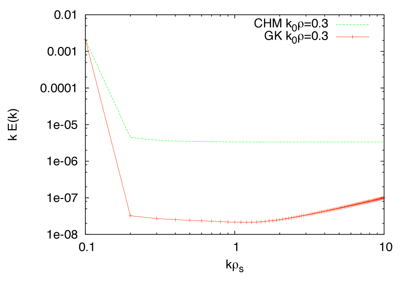
Figure 2: (Color online) Spectra for 2+1D gyrokinetics (GK) and for the Charney-Hasegawa-Mima (CHM) equations, corresponding to the model initial conditions with energy initially at $k_{0}\rho_{s}=0.3$. Both spectra show a significant transfer of energy to larger scales, resulting in a negative temperature state with most of the energy condensed into the longest wavelength in the domain.

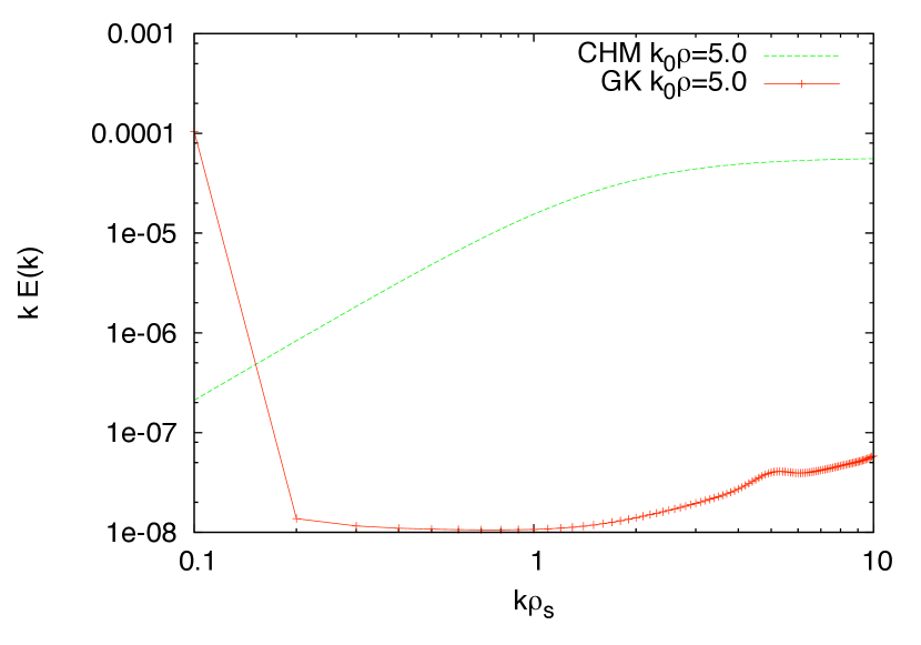
Figure 3: (Color online) Spectra for 2+1D gyrokinetics and Charney-Hasegawa-Mima, like Fig. (2) except the energy is initially at a higher wavenumber of $k_{0}\rho_{s}=5.0$.

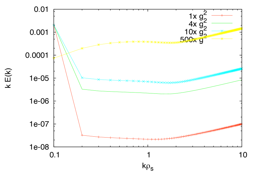
Figure 4: (Color online) Spectra for 2+1D gyrokinetics for initial conditions with the energy at $k_{0}\rho_{s}=0.3$ like Fig. (2), but with the value of the entropy invariants $G_{i}$ enhanced relative to the model initial conditions by factors of $1\times$, $4\times$, $10\times$, and $500\times$.

It is possible to increase the size of the tail in the 2+1D gyrokinetic spectrum by increasing the amplitude of the $G_{i}$ relative to the energy, as shown in Fig. (4). Considering a long-wavelength initial condition ignoring FLR effects, this can occur if a component is added to $g({\bf R},v,t=0)$ that oscillates in velocity so that it makes no contribution to the potential $\propto\int dvvg$, but does enhance $G_{i}=\int d^{2}R\,|g({\bf R},v_{i})|^{2}$. This can model the effects of temperature gradients in the background $F_{0}$ that drives the initial perturbation, or the build up of large values of $G_{i}$ in a long turbulence simulation without adequate dissipation because of the entropy balance relationships,Krommes94 ; Nevins05 thus leading to bottleneck problems.FrischPRL08 Note that the dependence of the tail on the enhancement of $G_{i}$ is a strongly nonlinear function. Note10 In the limit of very large $G_{i}/E$, the spectrum will approach equipartition among Fourier modes, $E\propto k$. One can also consider how the spectrum depends on the assumed velocity grid spacing $\Delta v$. From numerical results, confirmed by analytic scalings, one finds that as $\Delta v$ goes to zero, with fixed values of $E$ and $G_{i}$, that $\alpha_{0}\propto-1/\Delta v$ goes to negative infinity (while $\alpha_{i}\rightarrow$ constant for $i>0$), corresponding to a negative temperature state with all of the energy in the lowest $k$ mode, so $E(k)=0$ for all $k>k_{min}$.

Appendix E Thermal noise spectra in numerical schemes

In the 3+2D results in Sec. (II.2), we worked out the electrostatic spectrum, Eq. (16) and showed that the shape agrees with earlier results for the spectrum in a PIC code. Here we show that the magnitude agrees as well, with the proper relation between certain quantities in a continuum code and a PIC code. Begin by defining a weighted mean-square average of the distribution function $\overline{g^{2}}=\int d^{3}R\int d^{3}v\langle g^{2}\rangle/(F_{0}V)$ (an overbar is used here to indicate a combined velocity space average and an ensemble/volume average, to be distinguished from angle brackets that indicate an ensemble average). This uses the same velocity weighting as found in the $W_{g0}$ component of the generalized energy in Eq. (13). After discretization, this becomes $\overline{g^{2}}=2\tilde{\sum}_{\bf k}\sum_{i}m_{i}c_{i,i}({\bf k})/F_{0}({\bf v}_{i})$. Using Eq. (11) evaluated with the coefficients given just before Eq. (15) for the 3+2D case, and using the same approximations as used just before Eq. (16) (where velocity summations are approximated by integrals assuming a well-resolved velocity limit), one can show that

$$\overline{g^{2}}=\frac{2}{\gamma}\left(N\tilde{\sum}_{\bf k}-\tilde{\sum}_{\bf k}\Gamma_{0}(k_{\mbox{$\scriptscriptstyle\perp$}}^{2})\right)\approx\frac{NN_{k}}{\gamma},$$

for $N\gg 1$ (recall that $\tilde{\sum}_{\bf k}$ is defined as a sum over the modes in the upper half plane, so the total number of Fourier modes is $2\tilde{\sum}_{\bf k}=N_{k}$). We thus find that the thermal noise spectrum in Eq. (5) of Ref. Nevins05, for $\delta f$ PIC codes (using a weighted-particle Klimontovich representation for the distribution function) is identical to the thermal spectrum calculated here for a continuum code using a spectral representation for the distribution function, with the identification of $1/\gamma=\overline{g^{2}}/(NN_{k})$ in a continuum code with $\overline{w^{2}}/N_{p}$ in a PIC code. So the total number of particles $N_{p}$ in the PIC code is equivalent to $NN_{k}$, where $N$ is the number of velocity grid points and $N_{k}$ is the number of Fourier modes in the continuum code, and the mean squared particle weight $\overline{w^{2}}$ (which is called $\langle w^{2}\rangle$ in Ref. Nevins05, ) is equivalent to the continuum value of the mean-square particle distribution function $\overline{g^{2}}$. (From the PIC perspective, this is consistent because the particle weights $w$ are equivalent to $\delta f/F_{0}$, and in $\overline{w^{2}}=\sum_{i=1}^{N_{p}}\langle w_{i}^{2}\rangle/N_{p}$, the marker particles have an $F_{0}$ distribution.) This equivalence between continuum and PIC thermal spectra is similar to that found in 2-D hydrodynamics between Fourier-Galerkin and point-vortex representations of the problem. (The finite-size particles used in most plasma PIC codes provides a kind of ultraviolet cutoff that removes issues that could arise from point vortices or point particles forming tightly-bound pairs.)

The thermal noise spectrum in PIC codes can be worked out using the test-particle superposition principle, assuming that shielded test particles can be considered independent and random. The equivalence of the PIC and continuum thermal spectra indicates that one can likewise consider the random phase and amplitude of a Fourier-mode in $g$ at a particular velocity (plus the plasma shielding of this mode) to be like the random position and weight of a shielded test particle.

Since the thermal noise level $\langle{\mbox{$\varphi$}}^{2}\rangle=2\tilde{\sum}_{\bf k}\langle|\hat{\mbox{$\varphi$}}_{\bf k}|^{2}\rangle$ scales as $\overline{g^{2}}/N$, it is important for both PIC and continuum codes to either have enough particles or velocity grid points per spatial grid point so that the noise does not get too large on the time scale of the simulation, or to have enough small-scale dissipation to prevent the particle weights or $\overline{g^{2}}$ from growing too large during the simulation and causing a bottleneck problemFrischPRL08 or a numerical diffusion problem.Nevins05 (We have considered the uniform plasma case in this paper where $\overline{g^{2}}$ is a constant set by initial conditions, but in the case of turbulence driven by a background gradient, $\overline{g^{2}}$ will increase in time due to an entropy balance relationKrommes94 ; Nevins05 unless dissipation is accounted for.) Most continuum codes avoid such problems by employing either physical collisions or numerical dissipation such as high order upwinding or hyperdiffusion, though work on improved subgrid models might be able to help optimize the performance by reducing resolution requirements. While $\delta f$ PIC simulations can formally work correctly for a given simulation time period if enough particles are used, eventually the noise can grow in time to become a problem. PIC codes can avoid this issue and/or reduce the particle resolution requirements by employing weight-resetting methods,YChen08 which essentially provide some numerical diffusion to limit the growth of the weights.

References

- (1) E. Frieman and L. Chen, Phys. Fluids 25, 502 (1982).
- (2) W. W. Lee, Phys. Fluids 26, 556 (1983).
- (3) J. A. Brizard and T. S. Hahm, Review of Modern Physics 79, 421 (2007).
- (4) A. A. Schekochihin, S. C. Cowley, W. Dorland, G. W. Hammett, G. G. Howes, E. Quataert, and T. Tatsuno, Astrophys. J. Suppl. 182, 310 (2009).
- (5) G. G. Howes, S. C. Cowley, W. Dorland, G. W. Hammett, E. Quataert, and A. A. Schekochihin, Astrophys. J. 651, 590 (2006), http://arxiv.org/abs/astro-ph/0511812.
- (6) J. A. Krommes, Physica Scripta(2010), "Nonlinear gyrokinetics: A powerful tool for the description of microturbulence in magnetized plasmas", to be published.
- (7) U. Frisch, Turbulence: The Legacy of Kolmogorov (Cambridge University Press, 1995).
- (8) G. Eyink and K. Sreenivasan, Review of Modern Physics 78, 87 (2006).
- (9) T.-D. Lee, Q. Appl. Math. 10, 69 (1952).
- (10) R. H. Kraichnan and D. Montgomery, Rep. Prog. Phys. 43, 35 (1980).
- (11) J. B. Taylor, Plasma Phys. Control. Fusion 39, A1 (1997).
- (12) J. A. Krommes, Physics Reports 360, 1 (2002).
- (13) A. B. Langdon, Phys. Fluids 22, 163 (1979).
- (14) C. K. Birdsall and A. B. Langdon, Plasma Physics via Computer Simulation, (McGraw-Hill, New York, 1985).
- (15) J. Krommes, W. W. Lee, and C. Oberman, Physics of Fluids 29, 2421 (1986).
- (16) J. A. Krommes, Phys. Fluids B 5, 1066 (1993).
- (17) J. A. Krommes and S. Rath, Phys. Rev. E 67, 066402 (28 pages) (2003).
- (18) J. B. Taylor and B. McNamara, Phys. Fluids 14, 1492 (1971).
- (19) S. Edwards and J. B. Taylor, Proc. R. Soc. Lond. A. 336, 257 (1974).
- (20) D. Montgomery, L. Turner, Phys. Fluids 23, 265 (1980).
- (21) F. Y. Gang, B. D. Scott, P. H. Diamond, Phys. Fluids B 1, 1331 (1989).
- (22) J. B. Taylor, M. Borchardt, and P. Helander, Phys. Rev. Lett. 102, 124505 (2009).
- (23) H. Clercx, S. Maassen, and G. J. F. van Heijst, Phys. Rev. Lett. 80, 5129 (1998).
- (24) G. J. F. van Heijst and H. Clercx, Fluid Dyn. Res. 41, 064002 (2009).
- (25) J. E. Rice, J. of Physics: Conf. Series 123, 012003 (2008).
- (26) W. Solomon, K. Burrell, A. Garofalo, S. Kaye, R. Bell, A. Cole, J. deGrassie, P. Diamond, T. Hahm, G. Jackson, M. Lanctot, C. Petty, H. Reimerdes, S. Sabbagh, E. Strait, T. Tala, and R. Waltz, Phys. Plasmas 17, 156108 (2010).
- (27) R. H. Kraichnan, Physics of Fluids 10, 1417 (1967).
- (28) U. Frisch, A. Pouquet, J. Léorat, and A. Mazure, Journal of Fluid Mechanics 68, 769 (1975).
- (29) U. Frisch, S. Kurien, R. Pandit, W. Pauls, S. S. Ray, A. Wirth, and J.-Z. Zhu, Phys. Rev. Lett. 101, 144501 (2008).
- (30) J.-Z. Zhu and M. Taylor, Chinese Physics Letters 27, 054702 (2010).
- (31) J.-Z. Zhu, Phys. Rev. E 72, 026303 (2005).
- (32) S. Servidio, W. H. Matthaeus, and V. Carbone, Phys. Plasmas 15, 042314 (2008).
- (33) A. A. Schekochihin, S. C. Cowley, W. Dorland, G. W. Hammett, G. G. Howes, G. G. Plunk, E. Quataert, and T. Tatsuno, Plasma Phys. Control. Fusion 50, 124024 (2008).
- (34) W. M. Nevins, G. W. Hammett, A. M. Dimits, W. Dorland, and D. E. Shumaker, Phys. Plasmas 12, 122305 (2005).
- (35) G. Plunk, “The theory of gyrokinetic turbulence: A multiple-scales approach,” (2009), UCLA Ph.D. thesis, arxiv.org/abs/0903.1091.
- (36) G. Plunk, S. Cowley, A. Schekochihin, and T. Tatsuno, “Two-dimensional gyrokinetic turbulence,” To be published in The Journal of Fluid Mechanics. (see also: arXiv:0904.0243)(2009).
- (37) We acknowledge Drs. T.-S. Hahm and W. W. Lee for the interactions which help to write down this terse formula.
- (38) G. W. Hammett, M. A. Beer, W. Dorland, S. C. Cowley, and S. A. Smith, Plasma Phys. Control. Fusion 35, 973 (1993).
- (39) W. Dorland and G. W. Hammett, Phys. Fluids B 5, 812 (1993).
- (40) B. I. Cohen et al., Phys. Fluids B 5, 2967 (1993).
- (41) A. Dimits, T. Williams, J. Byers, and B. Cohen, Phys. Rev. Lett. 77, 71 (1996).
- (42) A. Dimits, G. Bateman, M. Beer, B. Cohen, W. Dorland, G. Hammett, C. Kim, J. Kinsey, M. Kotschenreuther, A. Kritz, L. Lao, J.Mandrekas, W. Nevins, S. Parker, A. Redd, D. Shumaker, R. Sydora, and J.Weiland, Phys. Plasmas 7, 969 (2000).
- (43) F. Jenko, W. Dorland, M. Kotschenreuther, and B. Rogers, Phys. Plasmas 7, 1904 (2000).
- (44) W. Dorland, F. Jenko, M. Kotschenreuther, and B. Rogers, Phys. Rev. Lett. 85, 5579 (2000).
- (45) Conceptually, as Eq. (6) is actually the Hankel transform, working in Hankel space and doing Hankel/Bessel Galerkin truncation, seems to be also attractive. However, due to the extra complication of the (modified) Bessel functions (series) and the inter-play of k and spaces, it is not yet clear how to proceed in that direction. Hankel Galerkin truncated absolute equilibrium may bring velocity-space insights; but, our analysis in Fourier space, with the velocity variable being integrated out, does not depend on the details of the treatment of velocity.
- (46) The formulation and calculation for the arbitrary (but integrable) velocity field or the continuous limits of the present calculations will involve some subtleties which are not essential to our main results here for a discretized velocity dimension, which is in any case needed for practical comparisons with numerical codes.
- (47) More general integration algorithms can be represented in this form, as the weights and grid points can be chosen to correspond to high-order Gaussian quadrature (as is done in present continuum codes,Kotschenreuther95 ) equivalent to a weighted orthogonal polynomial basis of degree (these weighted basis functions can cover the infinite velocity domain), providing super-exponential spectral accuracy with an error that asymptotically scales as for smooth solutions.
- (48) E. T. Jaynes, Phys. Rev. 106, 620 (1957).
- (49) E. T. Jaynes, Phys. Rev. 108, 171 (1957).
- (50) J.-Z. Zhu, “Dual cascade and its possible variations in magnetized kinetic plasma turbulence,” Submitted to Physics Review E; see also: arXiv:1008.0330.
- (51) A. Hasegawa and K. Mima, Phys. Fluids 21, 87 (1978).
- (52) J. Charney, J. Atmos. Sci. 28, 1087 (1971).
- (53) Hasegawa and Mima did not include the factor in the expression and thus neglected the enhancement of zonal flows by the lack of electron response to modes. There is ambiguity in how to treat modes in the quasi-2D limit where one does not directly keep track of the spectrum and does not know what fraction of the fluctuation energy is in modes that satisfy so that an adiabatic electron response can be used.
- (54) D. Fyfe and D. Montgomery, Phys. Fluids 22, 246 (1979).
- (55) T. Tatsuno, W. Dorland, A. A. Schekochihin, G. G. Plunk, M. Barnes, S. C. Cowley, and G. G. Howes, Phys. Rev. Lett. 103, 015003 (2009).
- (56) I. G. Abel, M. Barnes, S. C. Cowley, W. Dorland, and A. A. Schekochihin, Phys. Plasmas 15, 122509 (2008).
- (57) J. A. Krommes and G. Hu, Phys. Plasmas 1, 3211 (1994).
- (58) If a standard second order finite differencing is used in calculating the parallel electric field, then the finite differencing factor in Ref.(\rev@citealpnumNevins05) is given by , where is the parallel grid spacing, so for well resolved wave numbers. If a pseudo-spectral method is used to calculate in -space, then .
- (59) G. Hu and J. A. Krommes, Phys. Plasmas 1, 863 (1994).
- (60) B. N. Rogers, W. Dorland, and M. Kotschenreuther, Phys. Rev. Lett. 85, 5336 (2000).
- (61) P. Goldreich and S. Sridhar, ApJ 438, 763 (1995).
- (62) P. Goldreich and S. Sridhar, ApJ 485, 680 (1997).
- (63) J.-Z. Zhu, Chinese Physics Letters 23, 2139 (2006).
- (64) M. S. Bartlett, Annals of Mathematical Statistics 22, 107 (1951).
- (65) JZZ is not responsible for all the computations and discussions in this section. Especially, JZZ believes there are subtleties in taking the continuous limit which can be illustrated with the direct formulation and calculation for the problem with continuous velocity, which is consistent with the present calculation with discretization of (or quantized) velocity, as shown in Ref. Zhu20103, .
- (66) J. J. Moré, B. S. Garbow, and K. E. Hillstrom, “User Guide for MINPACK-1,” Argonne National Laboratory Report ANL-80-74 (1980), http://www.netlib.org/minpack (1999).
- (67) The isotropic energy spectra in these plots is defined as , where is angle-averaged by averaging over all such that . This avoids small fluctuations in the spectrum that could occur because the number of discrete Fourier modes that lie in the band fluctuates around .
- (68) Note that the -axis in these plots is , in order that the eye can more easily gauge regions of equal contribution to the total energy with a log -axis, since . For example, this extra factor of accounts for the fact that there are 10 times as many Fourier modes between and than between and .
- (69) The gyrokinetic case in Fig. (2) has , very close to the realizability limit . The values of were larger than the initial estimate of . For example, is times this estimate at the corresponding to .
- (70) For reference, the case in Fig. (4) with the increased by a factor of 400 still has a negative value of , with . The were all within 20% of the initial estimate of .
- (71) Y. Chen, S. E. Parker, G. Rewoldt, S. Ku, G. Y. Park, and C.-S. Chang, Phys. Plasmas 15, 055905 (2008).
- (72) M. Kotschenreuther, G. Rewoldt, and W. Tang, Comp. Phys. Comm. 88, 128 (1995).