Hindrance in the fusion of ⁴⁸Ca+⁴⁸Ca

Abstract

The coupled-channels technique is applied to analyze recent fusion data for ⁴⁸Ca+⁴⁸Ca. The calculations include the excitations of the low-lying $2^{+}$, $3^{-}$ and $5^{-}$ states in projectile and target, and the influence of mutual excitations as well as the two-phonon quadrupole excitations is also investigated. The ion-ion potential is obtained by double-folding the nuclear densities of the reacting nuclei with the M3Y+repulsion effective interaction but a standard Woods-Saxon potential is also applied. The data exhibit a strong hindrance at low energy compared to calculations that are based on a standard Woods-Saxon potential but they can be reproduced quite well by applying the M3Y+repulsion potential with an adjusted radius of the nuclear density. The influence of the polarization of high-lying states on the extracted radius is discussed.

I Introduction

Heavy-ion fusion reactions are sensitive probes of the nuclear surface of the reacting nuclei. Roughly speaking, the height of the Coulomb barrier is determined by the radii and diffuseness of the densities, and the enhancement of fusion at subbarrier energies is governed by couplings to the excitation of low-lying surface modes baha . This picture may not always succeed in reproducing the measured cross sections. In practical coupled-channels calculations it is often necessary to make adjustments, either in the structure input or in the ion-ion potential. The adjustments may reflect the influence of high-lying states or other reaction channels that are not treated explicitly in the calculations. Another complication is the hindrance of fusion which occurs at low energies and very small cross sections jiangsys . The hindrance can be explained, for example, by using a shallow potential in entrance channel misi75 or by modeling the fusion dynamics for touching and overlapping nuclei ichikawa .

In this work the coupled-channels technique is applied to analyze the fusion data for ⁴⁸Ca+⁴⁸Ca that were recently measured down to very small cross sections below 1 $\mu$b stef4848 . An analysis of the data provides the opportunity to investigate whether the fusion hindrance, which is a well established phenomenon in extreme subbarrier fusion reactions of medium-heavy systems with large negative Q-values jiangsys , also occurs in the fusion of calcium isotopes with near zero Q-values. An indication of a hindrance in the fusion of ⁴⁸Ca+⁴⁸Ca has already been observed stef4848 because the low-energy data could only be reproduced by coupled-channels calculations that employ a very large diffuseness of the ion-ion potential. However, the hindrance observed there was not strong enough to show an $S$ factor maximum in the energy region of the measurement.

The ion-ion potential and the nuclear couplings that will be used are derived as in previous work misi75 from the double-folding of the densities of the reacting nuclei and the M3Y+repulsion effective interaction. Since the low-lying structure of ⁴⁸Ca is fairly well established and the influence of transfer reactions is always suppressed for symmetric systems, it is expected that the simple picture of fusion described above would apply to the fusion of ⁴⁸Ca+⁴⁸Ca. On the other hand, it is well known that the excitation and/or polarization of high-lying states that are included explicitly in the coupled-channels calculations can lead to a negative energy shift of the calculated fusion cross sections takigawa . This is effectively equivalent to increasing the radii of the reacting nuclei. The radius that is extracted by optimizing the fit to the fusion data can therefore be too large because it can be contaminated by the polarization of states which are not included explicitly in the calculations. It is of interest to see how the extracted radius depends on the model space of excited states that are included in the calculations, and how well it compares to the expected matter radius of ⁴⁸Ca.

The study of the fusion of different calcium isotopes started more than twenty years ago with the measurements by Aljuwair et al. aljuwair but the cross sections were only measured down to about 1 mb. The most challenging theoretical issue at that time was to explain the fusion of ⁴⁰Ca+⁴⁸Ca which appeared to be strongly enhanced by couplings to transfer reactions, in particular to those with positive Q values landowne ; fricke . A strong motivation for reviving the study of the fusion of calcium isotopes is that, in addition to ⁴⁸Ca+⁴⁸Ca stef4848 , the fusion of ⁴⁰Ca+⁴⁸Ca has also recently been measured down to the 1 $\mu$b jiang4048 , and a new measurement for ⁴⁰Ca+⁴⁰Ca is underway stef4040 . In order to be able to focus on and isolate the effect of transfer on the fusion of the asymmetric ⁴⁰Ca+⁴⁸C system, it is necessary first to develop a good description of the fusion of the two symmetric systems, and the present work is a step in that direction.

The nuclear structure properties of ⁴⁸Ca are discussed in the next section and Sect. III describes the construction of the ion-ion potential. The coupled-channels technique is summarized in Sect. IV together with an analysis of the data that is based on Woods-Saxon potentials. The analysis based on the M3Y+repulsion potential is presented in Sect. V. Finally, the conclusions are given in Sect. VI.

II Nuclear structure input

The nuclear structure input to the coupled-channels calculations is shown in Table 1. The elastic channel and the one-phonon excitations of the low-lying $2^{+}$, $3^{-}$ and $5^{-}$ states in projectile and target results in a total of 7 channels.. The coupling strengths for the excitation of these states are taken from Ref. flem where they were calibrated by analyzing the elastic and inelastic scattering of ¹⁶O on calcium isotopes rehm . It should be noted that the Coulomb and nuclear coupling strengths, expressed in Table 1 by the values of $\beta R/\sqrt{4\pi}$, are different. The Coulomb couplings are in most cases consistent with the currently adopted electromagnetic transition probabilities or $B$-values ENDSF that are quoted in the third column of Table 1.

Also shown in Table 1 are the $0^{+}$, $2^{+}$ and $4^{+}$ members of two-phonon quadrupole excitation. The adopted $B(E2)$-values ENDSF shown in the third column of the second part of Table 1 can be combined into an effective two-phonon excitation. For example, the effective $B(E2)$ value for the two- to one-phonon transition is given by the sum,

$$B(E2,{\rm 2ph}\rightarrow{\rm 1ph})=\sum_{I=0,2,4}\langle 2020|I0\rangle^{2}\ B(E2,I\rightarrow 2),$$ (1)

and the two-phonon excitation energy is obtained as the weighted average of the individual two-phonon excitations energies prc72 . The parameters obtained for the effective two-phonon quadrupole excitation are shown in the last line of Table 1. Including the effective two-phonon quadrupole excitations in the coupled-channels calculations, in addition to the 7 channels mentioned above, leads to a total of 9 channels. Unfortunately, nothing is known about the two-phonon excitations of the $3^{-}$ and $5^{-}$ states so they will be ignored.

To get a feeling of the influence of higher-order excitations on the calculated fusion cross sections one can also include all of the 15 mutual excitations channels that are generated from the six one-phonon excitations presented in Table 1. Together with the basic 9 channels mentioned above, that sums up to a total of 24 channels. This will be referred to as the full calculation and the results will be compared to the fusion data and to calculations that include the 9 channels described above, as well as the no-coupling limit in which case there is only 1 channel.

Table 1: Nuclear structure input for ⁴⁸Ca. Values marked with * are from Ref. flem . The $B(E\lambda)$ values are from Ref, ENDSF . They are consistent with the Coulomb excitation parameters $(\beta R)_{C}/\sqrt{4\pi}$, except for the $3^{-}$ state where Ref. flem uses a larger value, $B(E3)$ = 6.8 W.u. The second part of the Table shows the 3 transitions that determine the effective two-phonon quadrupole state. Its excitation energy and couplings to the $2^{+}_{1}$ state are shown in the last line.

$I^{\pi}$	$E_{x}$ (MeV)	$B(E\lambda)$ (W.u.)	$\frac{(\beta R)_{C}}{\sqrt{4\pi}}$ (fm)	$\frac{(\beta R)_{N}}{\sqrt{4\pi}}$ (fm)
$2^{+}_{1}$	3.832	1.71(9)	0.126*	0.190*
$3^{-}$	4.507	5.0(8)	0.250*	0.190*
$5^{-}$	5.146		0.049*	0.038*
$0^{+}_{2}\rightarrow 2^{+}_{1}$	4.283	10.1(6)	[0.098]
$4^{+}_{1}\rightarrow 2^{+}_{1}$	4.503	0.261(6)	[0.025]
$2_{2}^{+}\rightarrow 2_{1}^{+}$	5.311	9(9)	[0.111]
Eff 2PH	4.849	4.7(29)	0.15	0.15

III The ion-ion potential

The parameters of the Woods-Saxon (WS) potentials that will be used in this work,

$$U_{\rm WS}(r)=\frac{-V_{0}}{1+\exp((r-R_{0})/a)},$$ (2)

are those proposed in Ref. BW , Eqs. (III.2.40-45). The parameters for the system ⁴⁸Ca+⁴⁸Ca are $a$ = 0.662 fm for the diffuseness and $V_{0}$ = 64.10 MeV for the depth of the potential. We refer to this potential as the ‘standard’ WS potential because its diffuseness is consistent with the analysis of elastic scattering data BW . The radius $R_{0}$, on the other hand, will be treated as a free parameter and it will be adjusted to optimize the fit to the data in the coupled-channels calculations that are discussed in the next section.

There is an interesting point concerning the isospin dependence of the nuclear potential proposed in Ref. BW . It enters through the average nuclear surface tension $\gamma$ of the reacting nuclei,

$$\gamma=0.95\Bigl{[}1-1.8\ \frac{N_{a}-Z_{a}}{A_{a}}\ \frac{N_{b}-Z_{b}}{A_{b}}\Bigr{]}\ \ {\rm MeV\ fm^{-2}},$$ (3)

according to Ref. BW , Eq. (III.2.30). The correction factor in Eq. (3), which depends on neutron excess, is equal to one in reactions that involve ⁴⁰Ca. In the case of ⁴⁸Ca+⁴⁸Ca, the correction factor reduces the surface tension by 5%; this correction is included in the value of the depth parameter $V_{0}$ mentioned above.

The M3Y+repulsion potential is calculated using the double-folding technique described in Ref. misi75 . It is based on the Reid parametrization of the M3Y effective nucleon-nulceon interaction bertsch . The spherical nuclear densities are parametrized by

$$\rho(r)=\frac{1}{2}\ \frac{\rho_{0}\exp(R/a)}{\cosh(r/a)+\cosh(R/a)},$$ (4)

where $R$ and $a$ are the radius and diffuseness parameters, respectively, and $\rho_{0}$ is a normalization constant. It is seen that the density, Eq. (4), approaches the Fermi function density $\rho_{0}/(1+\exp((r-R)/a))$ for $R/a>>1$. The parametrization Eq. (4) is used here because it has some very useful analytic properties as discussed in the Appendix of Ref. misopb . For example, the Fourier transform has an analytic form which simplifies the calculation of the double-folding potential in Fourier space from the expression misi75 ,

$$U(r)=\frac{1}{2\pi^{2}}\ \int k^{2}dk\ \rho(k)\ \rho(k)\ v_{nn}(k)\ j_{0}(kr),$$ (5)

where $v_{nn}(k)$ is the Fourier transform of the effective nucleon-nucleon interaction, and $j_{0}(x)=\sin(x)/x$ is a spherical Bessel function. Another advantage of the parametrization Eq. (4) is that the mean-square radius is given by the simple expression

$$\langle r^{2}\rangle=\frac{3}{5}\ \Bigl{(}R^{2}+\frac{7}{3}\ (a\pi)^{2}\Bigr{)}.$$ (6)

The repulsive part of the M3Y+repulsion potential is determined by two parameters, namely, the strength $v_{r}$ of the contact effective interaction,

$$v_{nn}^{\rm rep}({\bf r})=v_{r}\ \delta({\bf r}),$$ (7)

that generates it, and the diffuseness $a_{r}$ of the densities that are applied in the double-folding calculation misi75 . The radius parameter $R$ of the densities, on the other hand, is kept the same as in the calculation of the direct and the exchange parts of the M3Y double-folding potential. The diffuseness of the density that is used in calculating the direct and the exchange part of the M3Y potential is kept fixed with the value $a$ = 0.54 fm.

The two parameters $a_{r}$ and $v_{r}$ of the repulsive part of the potential are constrained so that total nuclear potential energy, $U_{N}(r)$, for completely overlapping nuclei is consistent with the equation-of-state. That leads to the relation misi75 ,

$$U_{N}(r=0)\approx\frac{A_{p}}{9}\ K,$$ (8)

where $A_{p}$ is the mass number of the smaller nucleus and $K$ is the nuclear incompressibility. For ⁴⁸Ca+⁴⁸Ca the value $K$ = 223.7 MeV predicted by the Thomas-Fermi model of Myers and Świa̧tecki myers will be used. Thus there are essentially only two free parameters of the M3Y+repulsion interaction, namely, the radius $R$ and the diffuseness parameter $a_{r}$. They will be adjusted to optimize the fit to the fusion data. The strength $v_{r}$ of the repulsive interaction, on the other hand, is constrained for given values of $R$ and $a_{r}$ by the nuclear incompressibility according to Eq. (8).

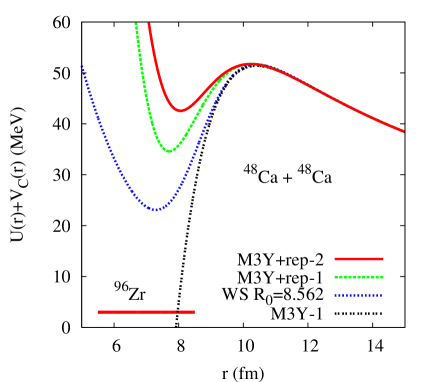
Figure 1: (Color online) Entrance channel potentials for ⁴⁸Ca+⁴⁸Ca obtained from the Woods-Saxon (WS, with $R_{0}$ = 8.562 fm) and the pure M3Y (M3Y-1) potentials. The two upper curves are the shallow M3Y+repulsion potentials determined in Sect. V. The energy of ground state of the compound nucleus ⁹⁶Zr is also indicated.

Some of the entrance channel potentials that are used in this work are illustrated in Fig. 1. The height of the Coulomb barrier is essentially the same for all four potentials but the thickness of the barrier is very different. The (blue) dashed curve is the entrance channel potential for the Woods-Saxon potential. It has the minimum pocket energy $V_{min}$ =23.09 MeV and the height of the Coulomb barrier is $V_{CB}$ = 51.63 MeV. The latter potential was determined by optimizing the fit to the fusion data with center-of-mass energy larger than 50 MeV. This energy cut was chosen because the fusion hindrance phenomenon sets in below 50 MeV as we shall see in the next section.

The upper two curves in Fig. 1 are the M3Y+repulsion entrance channel potentials that are obtained in Sect. V. They were determined by optimizing the fit to the fusion data in coupled-channels calculations that include the 24 channels described in Sect. II. There are two solutions, the M3Y+rep-1 and M3Y+rep-2 potentials, which are discussed in detail in Sect. V. These potentials are shallower than the standard Woods-Saxon potential, which is a characteristic feature of the M3Y+repulsion potentials that have been extracted from fusion data misi75 .

Finally, the entrance channel potential for the pure M3Y(+exchange) potential is also shown. It is unrealistic because it is deeper than the ground state energy of the compound nucleus ⁹⁶Zr which is indicated by the thick horizontal line.

IV Coupled-channels calculations

The coupled-channels calculations are performed in the rotating frame approximation, and the fusion cross sections are determined by imposing ingoing-wave boundary conditions at the position of the minimum of the pocket in the entrance potential. This procedure is commonly used and is described, for example, in Refs. misi75 ; oge . In the present work no imaginary potential will be applied. The fusion cross section will therefore vanish when the center-of-mass energies is lower than the minimum energy of the pocket in the entrance channel potential.

The nuclear potential enters the coupled equations both directly by determining the entrance channel potential and indirectly by determining the nuclear couplings to first and second order in the deformation amplitudes through the first and second derivatives of the nuclear potential (see Ref. oge for details.) There are in principle couplings of even higher order and to higher-lying states hagino but they will be ignored in the present study, partly because they are poorly known and partly because they are not expected to play a large role in the fusion of the not-so-heavy system ⁴⁸Ca+⁴⁸Ca. This expectation is based on the experience gained in Ref. prc72 . However, the polarization of high-lying states takigawa that are not included in the calculations could distort the analysis.

The fusion data for ⁴⁸Ca+⁴⁸Ca stef4848 are compared in Fig. 2 to two coupled-channels calculations that are based on standard Woods-Saxon potentials BW with the diffuseness $a$ = 0.662 fm and depth $V_{0}$ = 64.10 MeV. All 24 channels described in Sect. II were included in the calculations. It is seen that the data are hindered at low energies and the energy dependence is much steeper than predicted by the calculations. The dashed curve in Fig. 2 is the best fit to all data points; it is achieved with radius $R_{0}$ = 8.495 fm but the fit is very poor with an average $\chi^{2}$ per data point of $\chi^{2}/N$ = 7.9, including the statistical uncertainties and a systematic error of 7%.

The solid curve in Fig. 2 is based on the slightly larger radius, $R_{0}$ = 8.562 fm. It provides a better account of the data near and above the the Coulomb barrier as discussed below. The associated entrance channel potential is the (blue) dashed curve shown in Fig. 1.

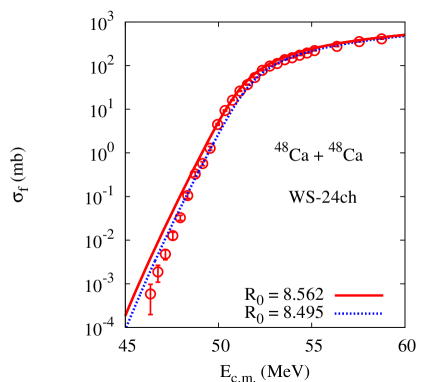
Figure 2: (Color online) Fusion cross sections for ⁴⁸Ca+⁴⁸Ca. The error bars reflect the statistical uncertainties. The curves are coupled-channels calculations with 24 channels that use Woods-Saxon (WS) potentials with two different radii.

The behavior of the hindrance in the fusion of ⁴⁸Ca+⁴⁸Ca is illustrated in Fig. 3 in terms of the ratio of the measured and calculated fusion cross sections. It is seen that the ratio with respect to the best fit to the data (the solid diamonds) has a strong peak near 50 MeV, slightly below the Coulomb barrier which is at $V_{CB}\approx$ 52 MeV. The ratio drops quickly at energies below 50 MeV. This is attributed to the fusion hindrance phenomenon. In fact, the steep falloff with decreasing energy observed in the comparison to standard coupled-channels calculations was the signature that was first used to identify the fusion hindrance jiangniy . Later it was shown that the hindrance is often so strong that the $S$ factor for fusion develops a maximum at very low energies. Moreover, it was realized that an $S$ factor maximum together with the energy $E_{S}$ of the maximum is a good quantitative way to characterize the fusion hindrance phenomenon jiang2004 .

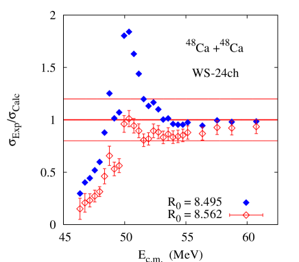
Figure 3: (Color online) Ratios of the measured and calculated cross sections shown in Fig. 2. The error bars on the open diamonds were determined by the statistical uncertainties and a 7% systematic error.

Since the fusion hindrance occurs at low energies one may exclude the low energy region and focus on reproducing the data at higher energies. The result of this approach is shown in Fig. 2 by the solid curve which is based on a slightly larger radius, $R_{0}$ = 8.562 fm. The larger radius implies larger cross sections below the Coulomb barrier but that gives a better description of the excitation function in the barrier region. The radius of the Woods-Saxon potential was therefore chosen so that the ratio of the measured and calculated cross sections essentially is a constant above 50 MeV. This is illustrated by the open diamonds Fig. 3. It is seen that the fusion hindrance sets in very strongly below 50 MeV, where the ratio falls off very steeply with decreasing energy.

V Analysis based on the M3Y+repulsion potential

The parameters of the M3Y+repulsion potential that provides the best fit to the data were determined using an improved calibration procedure. For a given nuclear radius parameter $R$ of ⁴⁸Ca and a given diffuseness $a_{r}$ of the density used in calculating the repulsive part of the potential, the strength of the repulsive term $v_{r}$ was adjusted so that the incompressibility $K$ = 223.7 MeV was achieved in Eq. (8). Having determined the nuclear potential, coupled-channels calculations were performed and the average $\chi^{2}$ per data point, $\chi^{2}/N$, was calculated from the statistical uncertainties and a systematic error of 7%.

The above procedure was repeated with different values of the radius $R$ for a fixed diffuseness parameter $a_{r}$ until a minimum $\chi^{2}/N$ was found. The whole process was repeated for a new value of $a_{r}$. The results of this process are illustrated in Fig. 4 where the $\chi^{2}/N$, minimized with respect to the radius $R$, is plotted as a function of the diffuseness parameter $a_{r}$. The dashed curve is the result of calculations that include the 9 channels. The solid curve is the result obtained with all 24 channels described in Sect. II.

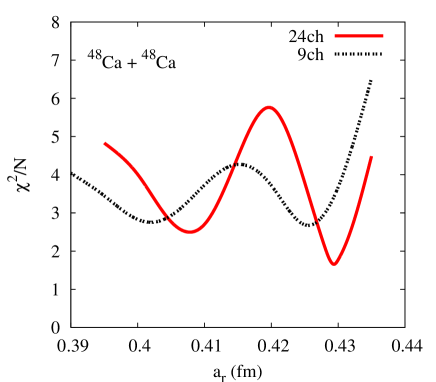
Figure 4: (Color online) Results of the $\chi^{2}$ analysis of the ⁴⁸Ca+⁴⁸Ca fusion data stef4848 . The $\chi^{2}/N$, minimized with respect to the radius $R$, is shown as function of the diffuseness parameter $a_{r}$. The solid curve (24ch) is for calculations that include 24 channels; the dashed curve (9ch) is for 9 channels.

The fusion data of Ref. stef4848 are compared in Fig. 5 to various calculations. The solid curve is the result of coupled-channels calculations associated with the deepest minimum in Fig. 4 which has a $\chi^{2}$ per data point of 1.66. The upper (blue) dashed curve is the cross sections obtained in similar calculations using the Woods-Saxon potential with the radius $R_{0}$ = 8.562 fm. All 24 channels described in Sect. II were included in both sets of calculations. The only difference between the two calculations is the choice of the nuclear potential, and it is seen that the shallow M3Y+repulsion potential labeled M3Y+rep-2 is a much better choice.

The lowest dashed curve in Fig. 5 is the cross section obtained in the no-coupling limit (i. e., with only 1 channel) using the same M3Y+repulsion potential that was used to produce the solid curve. Comparing the two curves, it is seen that the effect of the couplings to the 24 channels is equivalent to shifting the no-coupling limit almost 1 MeV to lower energies.

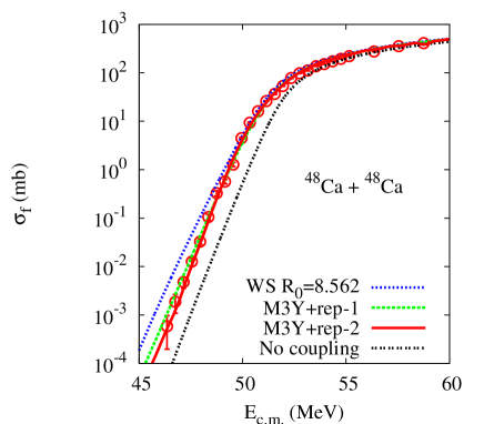
Figure 5: (Color online) Fusion cross sections for ⁴⁸Ca+⁴⁸Ca. The upper two curves are coupled-channels calculations with 24 channels that are based on the Woods-Saxon (WS) and the M3Y+repulsion (M3Y1+rep-1 and M3Y+rep-2) potentials discussed in the text. The lowest dashed curve is the no-coupling limit based on the same M3Y+repulsion potential.

V.1 Details of the analysis

The minima of the curves shown in Fig. 4 define the stable solutions of the $\chi^{2}$ analysis of the fusion data since they are minima with respect to variations in both $a_{r}$ and $R$. There are two local minima for each set of calculations and the parameters of the M3Y+repulsion interactions that determine them are given in Table 2. It is seen the two solutions obtained with 9 coupled have almost the same $\chi^{2}/N$. It is not clear what causes the existence of two solutions. The main difference between them is that the energy of pocket in the entrance channel potential, $V_{min}$, is about 8 MeV deeper in the solution with the smaller radius $R$.

Table 2: Parameters of the M3Y+repulsion potential associated with the $\chi^{2}$ minima in Fig. 4. Results are shown for coupled-channels calculations that include 9 and 24 channels, respectively. The last three columns show the minimum of the pocket $V_{min}$, the height of the Coulomb barrier $V_{CB}$, and the $\chi^{2}$ per data point.

No. of Ch.	$R$	$a_{r}$	$v_{r}$	$V_{min}$	$V_{CB}$	$\chi^{2}/N$
	(fm)	(fm)	(MeV fm3)	(MeV)	(MeV)
9	3.775	0.4025	480.1	33.58	51.67	2.76
9	3.810	0.4250	504.2	41.66	51.60	2.69
24	3.745	0.4070	481.8	34.61	51.77	2.52
24	3.798	0.4295	505.6	42.55	51.73	1.66

Of the two solutions obtained with 24 channels, the one with the larger radius gives a much better fit to the data with $\chi^{2}/N$ = 1.66 and the associated potential will be referred to as the M3Y+rep-2 potential. The potential for the solution with the smaller radius is called the M3Y+rep-1 potential. The two entrance channel potentials are illustrated in Fig. 1. An important question is whether the parameters of the stable solutions are realistic, or whether some of them can be ruled out as being unrealistic. One parameter of particular interest is the radius which is examined below.

The rms (root-mean-square) radii obtained for the stable solutions are shown in the fourth column of Table 3. They can be compared to the estimated experimental rms matter radius of ⁴⁸Ca shown in the last line of the Table. The estimate was based on the rms radius of the proton distribution, which was obtained from the measured rms charge radius angeli , and the experimental rms radius of the neutron distribution ray . The neutron radius is uncertain and several values exist in the literature. The experimental value chosen here was obtained from an analysis of elastic proton scattering data at 800 MeV ray and is in fairly good agreement with most of the theoretical predictions shown in Table 1 of Ref. dobi .

Table 3: The radius $R$ of ⁴⁸Ca extracted from the analysis of the fusion data; c. f. Table 2. The rms radii are compared to the measured rms charge angeli , proton angeli , and neutron ray radii. The latter two have been combined into the rms matter radius shown in the last line. The quoted matter-radius ([3.75] fm) was derived by inserting the rms matter-radius and the diffuseness $a$ = 0.54 fm into Eq. (6).

Reference	No of Ch.	$R$ (fm)	$\langle r^{2}\rangle^{1/2}$ (fm)
	9	3.755	3.547
	9	3.810	3.569
M3Y+rep-1	24	3.745	3.528
M3Y+rep-2	24	3.798	3.562
Charge angeli			3.474(1)
protons			3.387(1)
neutrons ray			3.63(5)
matter		[3.75]	3.53(3)

The estimated rms matter radius quoted in the last line of Table 3 is in perfect agreement with the rms radius associated with the M3Y+rep-1 solution. The rms radius for the M3Y+rep-2 solution is larger but it is still consistent with the experimental estimate within the 1$\sigma$ uncertainty. A possible explanation for the larger radius could be the influence of the polarization of high-lying states not included in the calculations (see below.)

It is also encouraging that the extracted values of $a_{r}$ shown in Table 2 are similar to those determined in the analysis of the fusion data for ⁶⁴Ni+⁶⁴Ni ($a_{r}$ = 0.403 fm misi75 ), ¹⁶O+¹⁶O ($a_{r}$ = 0.41 fm o16 ) and ⁴⁸Ca+⁹⁶Zr ($a_{r}$ = 0.40 fm ca48zr .) It is noted that in the previous works the densities (including the radius) were kept fixed and only the value of $a_{r}$ was adjusted in each case to improve the fit to the data.

V.2 Polarization effects

The polarization effect discussed in the introduction section is illustrated in Table 4. The Table shows that for the M3Y+rep-2 potential, one needs to shift the 1 channel calculation by $\Delta E$ = -0.80 MeV and the 9 channel calculation by -0.12 MeV in order to optimize the fit to the data. The negative energy shifts are equivalent to using a larger radius of the reacting nuclei. For example, the required energy shift of -0.12 MeV for the calculations with 9 channels can be simulated by increasing the radius of ⁴⁸Ca by only 0.02 fm.

The required energy shift $\Delta E$ shown in Table 4 for the calculation with 24 channels is zero simply because the radius $R$ was already adjusted in this case to optimize the fit to the data. The issue whether the calculations have converged with respect to the excitation and polarization of high-lying states is a difficult question to answer. It is possible that the polarization of other high-lying states, which have not been considered here, could play a role and explain part of the 0.05 fm difference between the radius of the M3Y+rep-2 solution and the estimated experimental matter radius (see Table 3.)

Table 4: The $\chi^{2}/N$ (column 3) obtained in calculations that use the M3Y+rep-2 potential and include 1, 9 or 24 channels. The energy shift $\Delta E$ of the calculations that optimizes the fit to the data, and the associated $\chi^{2}/N$, are shown in the last two columns.

$R$ (fm)	channels	$\chi^{2}/N$	$\Delta E$ (MeV)	$\chi^{2}/N$
3.798	1	33.3	-0.80	4.65
3.798	9	4.28	-0.12	2.71
3.798	24	1.66	0.0	1.66

V.3 $S$ factor representation

A good way to illustrate the behavior of the fusion cross section $\sigma_{f}$ at low energies is to plot the $S$ factor for fusion,

$$S=E_{c.m.}\ \sigma_{f}\ \exp(\eta-\eta_{0}),$$ (9)

where $\eta=Z_{1}Z_{2}e^{2}/(\hbar v)$ is the Sommerfeld parameter and $\eta_{0}$ is that value of $\eta$ at a fixed reference energy $E_{0}$. The $S$ factors for the fusion cross sections shown in Fig. 5 are illustrated in Fig. 6 using the (arbitrary) reference energy $E_{0}$ = 52 MeV. Also shown is the result obtained with the M3Y+rep-1 potential and 24 coupled channels.

The coupled-channels calculations for the Woods-Saxon potential produce an $S$ factor in Fig. 6 that keeps increasing with decreasing energy. The $S$ factors obtained with the two M3Y+repulsion potentials and 24 coupled channels are lower. The $S$ factor for best fit to the data (the solid curve, obtained with the M3Y+rep-2 potential) has a maximum at $E_{s}$ = 43.2 MeV. The cross section associated with the latter maximum is very small, about 0.3 nb. The $S$ factor for the calculation based on the M3Y+rep-1 potential has a maximum at $E_{s}$ = 35.4 MeV which is outside the depicted energy range.

It would be very interesting to know whether the predicted $S$ factor maximum near $E_{s}$ = 43.2 MeV can be confirmed by experiments but to measure a cross section of only 0.3 nb would be a serious challenge.

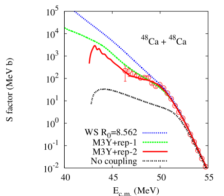
Figure 6: (Color online) $S$ factors for the fusion cross sections shown in Fig. 5. Also shown is the $S$ factor obtained in calculations with the M3Y+rep-1 potential. All calculations include 24 channels, except the no-coupling limit which has only 1 channel.

V.4 Logarithmic derivative

The logarithmic derivative of the energy-weighted cross sections,

$$L(E_{c.m.})=\frac{d}{dE_{c.m.}}\ln\Bigl{(}E_{c.m}\sigma_{f}\Bigr{)},$$ (10)

is illustrated in Fig. 7. The logarithmic derivatives derived from the data and from the coupled-channels calculation based on the M3Y+rep-2 potential (the solid curve) are seen to be in very good agreement. Similar results were obtained in Ref. stef4848 in coupled-channels calculations that used a Woods-Saxon potential with the large diffuseness $a$ = 0.9 fm. Thus it appears that a large diffuseness of the Woods-Saxon has an effect that is similar to that of the shallow M3Y+repulsion potential, at least in the low-energy region discussed here.

The similarity of the M3Y+repulsion and a Woods-Saxon potential was recently pointed out in Ref. godsi . It was shown that the M3Y+repulsion potential can be reproduced accurately in the barrier region by a Woods-Saxon potential with large diffuseness. However, a nuclear potential with a large diffuseness is inconsistent with many measurements of elastic and quasielastic scattering. For example, a recent systematic study of the quasielastic scattering of nuclei showed that a realistic diffuseness in the range of 0.64 to 0.69 fm is indeed required cjlin .

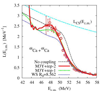
Figure 7: (Color online) The logarithmic derivative of the energy weighted cross sections shown in Fig. 5. Also shown is the result of coupled-channels calculations based on the M3Y+rep-1 potential. The top curve is the constant $S$ factor limit, $L_{CS}(E_{c.m.})$.

It is very interesting to point out that the low-energy behavior of the experimental logarithmic derivative shown in Fig. 7 is different from the behavior observed in other systems, in particular in medium-heavy systems jiangsys , where the logarithmic derivative usually increases linearly with decreasing energy and intersects with the logarithmic derivative for constant $S$ factor jiang2004 ,

$$L_{CS}(E_{c.m.})=\pi\eta/E_{c.m.}.$$ (11)

However, there are other systems that exhibit a deviant behavior at low energies. For example, the logarithmic derivative for the fusion of ³⁶S+⁴⁸Ca sca48 also becomes rather flat at low energies and it seems unlikely it will intersect with the constant $S$ factor limit. In fact, the $S$ factor for the fusion of ³⁶S+⁴⁸Ca increases slowly and linearly in a logarithmic plot with decreasing energy (see Fig. 3 of Ref. sca48 .)

Another interesting point is that the solid curve in Fig. 7 exhibits a maximum near 48 MeV before it rises steeply below 44 MeV. It intersects with the constant $S$ factor limit at $E_{s}$ = 43.2 MeV, where the associated $S$ factor in Fig. 6 develops a maximum.

VI Conclusions

The fusion data for ⁴⁸Ca+⁴⁸Ca have been analyzed using the coupled-channels technique and different ion-ion potentials. The analysis based on a standard Woods-Saxon potential clearly showed that the data are strongly hindered at low energies. By employing and adjusting the M3Y+repulsion double-folding potential it was possible to achieve an excellent description of the data.

The best fit to the data was achieved with a nuclear radius of ⁴⁸Ca that is slightly larger than but still consistent with the matter radius of ⁴⁸Ca. The latter radius was determined from the measured rms charge radius and the rms neutron radius extracted from an analysis of elastic proton scattering data. The fact that the extracted radius is slightly larger than the matter radius may be caused by the polarization of high-lying states that are not included in the coupled-channels calculations.

The entrance channel potential for the best fit to the data has a rather shallow pocket, consistent with the findings of previous analyses of fusion data for medium-heavy systems. The M3Y+repulsion potential model is therefore also referred to as the shallow potential model, in contrast to models based on the standard Woods-Saxon potentials, which have relatively deep pockets in the entrance channel potential.

The $S$ factor for the fusion of ⁴⁸Ca+⁴⁸Ca does not show a maximum within the energy range of the experiment. However, it is predicted to develop a maximum at a 3 MeV lower energy which is nearly the same as the energy value obtained from the extrapolation method in Ref. jiang4048 . The cross section associated with the maximum $S$ factor is very small ($\approx$ 0.3 nb) and is a serious challenge to the experimental technology.

Acknowledgments. One of the authors (H.E.) acknowledges discussions with Ş. Mişicu about double-folding potentials. This work was supported by the U.S. Department of Energy, Office of Nuclear Physics, contract no. DE-AC02-06CH11357.

References

- (1) A. B. Balantekin and N. Takigawa, Rev. Mod. Phys. 70, 77 (1998).
- (2) C.L. Jiang, B.B. Back, H. Esbensen, R.V.F Janssens, and K.E. Rehm, Phys. Rev. C 73, 014613 (2006).
- (3) Ş. Mişicu and H. Esbensen, Phys. Rev. C 75, 034606 (2007).
- (4) T. Ichikawa, K. Hagino, and A. Iwamoto, Phys. Rev. C 75, 064612 (2007); Phys. Rev. Lett. 103, 202701 (2009).
- (5) A. M. Stefanini et al.; Phys. Lett. B679, 95 (2009).
- (6) K. Hagino, N. Takigawa, and A. B. Balantekin, Phys. Rev. C 56, 2104 (1997).
- (7) H. A. Aljuwair et al., Phys. Rev. C 30, 1223 (1984).
- (8) S. Landowne, C. H. Dasso, R. A. Broglia, and G. Pollarolo, Phys. Rev. C 31, 1047 (1985).
- (9) H. Esbensen, S. H. Fricke, and S. Landowne, Phys. Rev. C 40, 2046 (1989).
- (10) C. L. Jiang et al., Phys. Rev. C 82, 041601(R) (2010).
- (11) A. M. Stefanini (private communications, 2010).
- (12) H. Esbensen and F. Videbaek, Phys. Rev. C 40, 126 (1989).
- (13) K. E. Rehm, W. Henning, J. R. Erskine, D. G. Kovar, M. H. Macfarlane, S. C. Pieper, and M. Rhoades-Brown, Phys. Rev. C 25, 1915 (1982).
- (14) Evaluated Nuclear Structure Date Files, National Nuclear Data Center, Brookhaven National Laboratory; http://www.nndc.bnl.gov/
- (15) H. Esbensen, Phys. Rev. C 72, 054607 (2005).
- (16) R. A. Broglia and A. Winther, Frontiers in Physics Lecture Notes Series: Heavy-ion Reactions (Addison-Wesley, Redwood City, CA, 1991). Vol. 84.
- (17) G. Bertsch, J. Borysowitcz, H. McManus, and W. G. Love, Nucl. Phys. A284, 399 (1977).
- (18) H. Esbensen and Ş. Mişicu, Phys. Rev. C 76, 054609 (2007).
- (19) W. D. Myers and W. J. Świa̧tecki, Phys. Rev. C 57, 3020 (1998).
- (20) H. Esbensen, Phys. Rev. C 68, 034604 (2003).
- (21) K. Hagino, N. Takigawa, M. Dasgupta, D. J. Hinde, and J. R. Leigh, Phys. Rev. C 55, 276 (1997).
- (22) C. L. Jiang et al., Phys. Rev. Lett. 89, 052701 (2002).
- (23) C. L. Jiang, H. Esbensen, B. B. Back, R. V. F. Janssens, and K. E. Rehm, Phys. Rev. C 69, 014604 (2004)
- (24) I. Angeli, Atomic Data Nuclear Data Tables 87, 185 (2004).
- (25) L. Ray, Phys. Rev. C 19, 1855 (1979).
- (26) J. Dobaczewski, W. Nazarewicz, and T. R. Werner, Zeit. für Phys. A 354, 27 (1996).
- (27) H. Esbensen, Phys. Rev. C 77, 054608 (2008).
- (28) H. Esbensen and C. L. Jiang, Phys. Rev. C 79, 064619 (2009).
- (29) O. N. Godsi and V. Zanganeh, Nucl. Phys. A846, 40 (2010).
- (30) C. J. Lin, H. M. Jia, H. Q. Zhang, F. Yang, X. X. Xu, F. Jia, Z. H. Liu, and K. Hagino, Phys. Rev. C 79, 064603 (2009).
- (31) A. M. Stefanini et al., Phys. Rev. C 78, 044607 (2008).