In All Likelihood, Deep Belief Is Not Enough
Abstract
Statistical models of natural stimuli provide an important tool for researchers in the fields of machine learning and computational neuroscience. A canonical way to quantitatively assess and compare the performance of statistical models is given by the likelihood. One class of statistical models which has recently gained increasing popularity and has been applied to a variety of complex data are deep belief networks. Analyses of these models, however, have been typically limited to qualitative analyses based on samples due to the computationally intractable nature of the model likelihood. Motivated by these circumstances, the present article provides a consistent estimator for the likelihood that is both computationally tractable and simple to apply in practice. Using this estimator, a deep belief network which has been suggested for the modeling of natural image patches is quantitatively investigated and compared to other models of natural image patches. Contrary to earlier claims based on qualitative results, the results presented in this article provide evidence that the model under investigation is not a particularly good model for natural images.
1 Introduction
Statistical models of naturally occurring stimuli constitute an important tool in machine learning and computational neuroscience, among many other areas. In machine learning, they have been applied both to supervised and unsupervised problems, such as denoising (e.g., Lyu and Simoncelli, 2007), classification (e.g., Lee et al., 2009) or prediction (e.g., Doretto et al., 2003). In computational neuroscience, statistical models have been used to analyze the structure of natural images as part of the quest to understand the tasks faced by the visual system of the brain (e.g., Lewicki and Doi, 2005; Olshausen and Field, 1996). Other examples include generative statistical models studied to derive better models of perceptual learning. Underlying these approaches is the assumption that the low-level areas of the brain adapt to the statistical structure of their sensory inputs and are less concerned with goals of behavior.
An important measure to assess the performance of a statistical model is the likelihood which allows us to objectively compare the density estimation performance of different models. Given two model instances with the same prior probability and a test set of data samples, the ratio of their likelihoods already tells us everything we need to know to decide which of the two models is more likely to have generated the dataset. Furthermore, for densities and , the negative expected log-likelihood represents the cross-entropy (or expected log-loss) term of the Kullback-Leibler (KL) divergence,
which is always non-negative and zero if and only if and are identical. The main motivation for the KL-divergence stems from coding theory, where the cross-entropy represents the coding cost of encoding samples drawn from with a code that would be optimal for samples drawn from . Correspondingly, the KL-divergence represents the additional coding cost created by using an optimal code which assumes the distribution of the samples to be instead of . Finally, the likelihood allows us to directly examine the success of maximum likelihood learning for different training settings. Unfortunately, for many interesting models, the likelihood is intractable to compute exactly.
One such class of models which has attracted a lot of attention in recent years is given by deep belief networks. Deep belief networks are hierarchical generative models introduced by Hinton et al. (Hinton and Salakhutdinov, 2006) together with a greedy learning rule as an approach to the long-standing challenge of training deep neural networks, that is, hierarchical neural networks with many layers. In supervised tasks, they have been shown to learn representations which can be successfully employed in classification tasks, such as character recognition (Hinton et al., 2006a) and speech recognition (Mohamed et al., 2009). In unsupervised tasks, where the likelihood is particularly important, they have been applied to a wide variety of complex datasets, such as patches of natural images (Osindero and Hinton, 2008; Ranzato et al., 2010; Ranzato and Hinton, 2010; Lee and Ng, 2007), motion capture recordings (Taylor et al., 2007) and images of faces (Susskind et al., 2008).
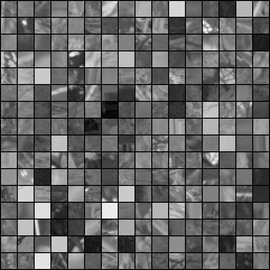
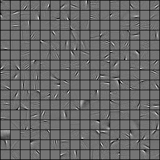
When applied to natural images, deep belief networks have been shown to develop biologically plausible features (Lee and Ng, 2007) and samples from the model were shown to adhere to certain statistical regularities also found in natural images (Osindero and Hinton, 2008). Examples of natural image patches and features learned by a deep belief network are presented in Figure 1.
In this article, after reviewing the relevant aspects of deep belief networks, we will derive a consistent estimator for its likelihood and demonstrate the estimator’s applicability in practice by evaluating a model trained on natural image patches. After a thorough quantitative analysis, we will argue that the deep belief network under consideration is not a particularly good model for estimating the density of small natural image patches, as it is outperformed with respect to the likelihood even by simple mixture models. Furthermore, we will show that adding layers to the network has only a small effect on the overall performance of the model if each layer is trained well enough and will offer a possible explanation for this observation by analyzing a best-case scenario of the greedy learning procedure commonly used for training deep belief networks.
2 Models
In this chapter we will review the statistical models used in the remainder of this article. In particular, we will describe the restricted Boltzmann machine (RBM) and some of its variants which constitute the main building blocks for constructing deep belief networks (DBNs). Furthermore, we will discuss some of the models’ properties relevant for estimating the likelihood of DBNs. Readers familiar with DBNs might want to skip this section or skim it to get acquainted with the notation.
Throughout this article, the goal of applying statistical models is assumed to be the approximation of a particular distribution of interest—often called the data distribution. We will denote this distribution by .
2.1 Boltzmann Machines
A Boltzmann machine is a potentially fully connected undirected graphical model—or Markov random field—with binary random variables. Its probability mass function is a Boltzmann distribution over binary states which is defined in terms of an energy function ,
| (1) |
where is given by
| (2) |
and depends on a symmetric weight matrix with zeros on the diagonal, i.e. for all , and bias terms . is called partition function and ensures the normalization of . In the following, unnormalized distributions will be marked with an asterisk:
Samples from the Boltzmann distribution can be obtained via Gibbs sampling, which operates by conditionally sampling each univariate random variable until some convergence criterion is reached. From definitions (1) and (2) it follows that the conditional probability of a unit being on given the states of all other units is given by
where is the sigmoidal logistic function. The Boltzmann machine can be seen as a stochastic generalization of the binary Hopfield network, which is based on the same energy function but updates its units deterministically using a step function, i.e. a unit is set to 1 if and set to 0 otherwise. In the limit of increasingly large weight magnitudes, the logistic function becomes a step function and the deterministic behavior of the Hopfield network can be recovered with the Boltzmann machine (Hinton, 2007).
Of particular interest for building DBNs are latent variable Boltzmann machines, that is, Boltzmann machines for which the states are only partially observed (Figure 2). We will refer to states of observed—or visible—random variables as and to states of unobserved—or hidden—random variables as , such that can be written as .
Approximation of the data distribution with the model distribution via maximum likelihood (ML) learning can be implemented by following the gradient of the model log-likelihood. In Boltzmann machines, this gradient is conceptually simple yet computationally very hard to evaluate. The gradient of the expected log-likelihood with respect to some parameter of the energy function is (Salakhutdinov, 2009):
| (3) |
The first term on the right-hand side of this equation is the expected gradient of the energy function when both hidden and observed states are sampled from the model, while the second term is the expected gradient of the energy function when the hidden states are drawn from the conditional distribution of the model, given a visible state drawn from the data distribution. Following this gradient increases the energy of the states which are more likely with respect to the model distribution and decreases the energy of the states which are more likely with respect to the data distribution. Remember that by the definition of the model (1), states with higher energy are less likely than states with lower energy.
As an example, the gradient of the log-likelihood with respect to the weight connecting a visible unit and a hidden unit becomes
A step in the direction of this gradient can be interpreted as a combination of Hebbian and anti-Hebbian learning (Hinton, 2003), where the first term corresponds to Hebbian learning and the second term to anti-Hebbian learning, respectively.
Evaluating the expectations, however, is computationally intractable for all but the simplest networks. Even approximating the expectations with Monte Carlo methods is typically very slow (Long and Servedio, 2010). Two measures can be taken to make learning in Boltzmann machines feasible: constraining the Boltzmann machine in some way, or replacing the likelihood with a simpler objective function. The former approach led to the introduction of RBMs, which will be discussed in the next section. The latter approach led to the now widely used contrastive divergence (CD) learning rule (Hinton, 2002) which represents a tractable approximation to ML learning: In CD learning, the expectation over the model distribution is replaced by an expectation over
from which samples are obtained by taking a sample from the data distribution, updating the hidden units, updating the visible units, and finally updating the hidden units again, while in each step keeping the respective set of other variables fixed. This corresponds to a single sweep of Gibbs sampling through all random variables of the model plus an additional update of the hidden units. If instead sweeps of Gibbs sampling are used, the learning procedure is generally referred to as CD() learning. For , ML learning is regained (Salakhutdinov, 2009).
2.2 Restricted Boltzmann Machines
A restricted Boltzmann machine (RBM) (Smolensky, 1986) is a Boltzmann machine whose energy function is constrained such that no direct interaction between two visible units or two hidden units is possible,
The corresponding graph has no connections between the visible units and no connections between the hidden units and is hence bipartite (Figure 2). The weight matrix is different to the one in equation (2) in that it now only contains interaction terms between the visible units and the hidden units and therefore no longer needs to be symmetric or constrained in any other way. Despite these constraints it has been shown that RBMs are universal approximators, i.e. for any distribution over binary states and any , there exists an RBM with a KL-divergence which is smaller than (Roux and Bengio, 2008).
In an RBM, the visible units are conditionally independent given the states of the hidden units and vice versa. The conditional distribution of the hidden units, for instance, is given by
where is the logistic sigmoidal function and is the -th column of . This allows for efficient Gibbs sampling of the model distribution (since one set of variables can be updated in parallel given the other) and thus for faster approximation of the log-likelihood gradient. Moreover, the unnormalized marginal distributions and of RBMs can be computed analytically by integrating out the respective other variable. For instance, the unnormalized marginal distribution of the visible units becomes
| (4) |
Two other models which can be used for constructing DBNs are the Gaussian RBM (GRBM) (Salakhutdinov, 2009) and the semi-restricted Boltzmann machine (SRBM) (Osindero and Hinton, 2008). The GRBM employs continuous instead of binary visible units (while keeping the hidden units binary) and can thus be used to model continuous data. Its energy function is given by
| (5) |
A somewhat more general definition allows a different for each individual visible unit (Salakhutdinov, 2009). As for the binary Boltzmann machine, training of the GRBM proceeds by following the gradient given in equation (3), or an approximation thereof. Its properties are similar to that of an RBM, except that its conditional distribution is a multivariate Gaussian distribution whose mean is determined by the hidden units,
Each state of the hidden units encodes one mean. controls the variance of each Gaussian and is the same for all states of the hidden units. The GRBM can therefore be interpreted as a mixture of an exponential number of Gaussian distributions with fixed, isotropic covariance and parameter sharing constraints.
In an SRBM, only the hidden units are constrained to have no direct connections to each other while the visible units are unconstrained (Figure 2). Importantly, analytic expressions are therefore only available for but not for . Furthermore, is no longer factorial. For efficiently training DBNs, conditional independence of the hidden units is more important than conditional independence of the visible units (Osindero and Hinton, 2008). This is in part due to the fact that the second-term on the right-hand side of equation (3) can still efficiently be evaluated if the hidden units are conditionally independent, and in part due to the way inference is done in DBNs.
2.3 Deep Belief Networks
DBNs (Hinton and Salakhutdinov, 2006) are hierarchical generative models composed of several layers of RBMs or one of their generalizations. While DBNs have been widely used as part of a heuristic for learning multiple layers of feature representations and for pretraining multi-layer perceptrons (by initializing the multi-layer perceptron with the parameters learned by a DBN), the existence of an efficient learning rule has made them become attractive also for density estimation tasks.
For simplicity, we will begin by defining a two-layer DBN. Let and be the densities of two RBMs over visible states and hidden states and . Then, the joint probability mass function of a two-layer DBN is defined to be
| (6) |
Interestingly, the resulting distribution is best described not as a deep Boltzmann machine, as one might expect, or even an undirected graphical model, but as a graphical model with undirected connections between and and directed connections between and (Figure 3). This characteristic of the model becomes evident in the generative process. A sample from the model can be drawn by first Gibbs sampling the distribution of the top layer to produce a state for . Afterwards, a sample is drawn from the much simpler distribution .
The definition can easily be extended to DBNs with three or more layers by replacing with , where is the marginal distribution of another RBM. Thus, by adding additional layers to the DBN, the prior distribution over the top-level hidden units— for the model defined in equation —is effectively replaced with a new prior distribution—in this case . DBNs with an arbitrary number of layers, like RBMs, have been shown to be universal approximators even if the number of hidden units in each layer is fixed to the number of visible units (Sutskever and Hinton, 2008). As mentioned earlier, another possibility to generalize DBNs is to allow for more general models as layers. One such model is the SRBM, which can model more complex interactions by having less restrictive independce assumptions. Alternatively, one could allow for models with units whose conditional probability distributions are not just binary, but can be any exponential family distribution (Welling et al., 2005)—one instance being the GRBM.
The greedy learning procedure (Hinton et al., 2006a) used for training DBNs starts by fitting the first-layer RBM (the one closest to the observations) to the data distribution. Afterwards, the prior distribution over the hidden units defined by the first layer, , is replaced by the marginal distribution of the second layer, , and the parameters of the second layer are trained by optimizing a lower bound to the log-likelihood of the two-layer DBN. In the following, we will derive this lower bound.
Let be a parameter of . The gradient of the log-likelihood with respect to is
| (7) |
Approximate ML learning could therefore in principle be implemented by training the second layer to approximate the posterior distribution using CD learning or a similar algorithm. However, exact sampling from the posterior distribution is difficult, as its evaluation involves integrating over an exponential number of states,
In order to make the training feasbile again, the posterior distribution is replaced by the factorial distribution . Training the DBN in this manner optimizes a variational lower bound on the log-likelihood,
| (8) | ||||
| (9) |
where (8) follows from Bayes’ theorem, (9) is due to Jensen’s inequality and is constant in , as only depends on . Taking the derivative of (9) with respect to yields with the posterior distribution replaced by . The greedy learning procedure can be generalized to more layers by training each additional layer to approximate the distribution obtained by conditionally sampling from each layer in turn, starting with the lowest layer.
3 Likelihood Estimation
In this section, we will discuss the problem of estimating the likelihood of a two-layer DBN with joint density
| (10) |
That is, for a given visible state , to estimate the value of
As we will see later, this problem can easily be generalized to more layers. As before, and refer to the densities of two RBMs.
Two difficulties arise when dealing with this problem in the context of DBNs. First, depends on a partition function whose exact evaluation requires integration over an exponential number of states. Second, despite our ability to integrate analytically over , even computing just the unnormalized likelihood still requires integration over an exponential number of hidden states ,
After briefly reviewing previous approaches to resolving these difficulties, we will propose an unbiased estimator for , its contribution being a possible solution to the second problem, and discuss how to construct a consistent estimator for based on this estimator. Finally, we will demonstrate its applicability to more general DBNs.
3.1 Previous Work
3.1.1 Annealed Importance Sampling
Salakhutdinov and Murray (2008) have shown how annealed importance sampling (AIS) (Neal, 2001) can be used to estimate the partition function of a restricted Boltzmann machine. Since our estimator will also rely on AIS estimates of the partition function, we will shortly describe the procedure here.
Importance sampling is a Monte Carlo method for unbiased estimation of expectations (MacKay, 2003) and is based on the following observation: Let be a density with whenever and let , then
| (11) |
for any function . is called the proposal distribution and is called importance weight. For , we get
| (12) |
Estimates of the partition function can therefore be obtained by drawing samples from a proposal distribution and averaging the resulting importance weights . It was pointed out in (Minka, 2005) that minimizing the variance of the importance sampling estimate of the partition function (12) is equivalent to minimizing an -divergence111With . -divergences are a generalization of the KL-divergence. between the proposal distribution and the true distribution . Therefore, for the estimate to work well in practice, should be both close to and easy to sample from.
Annealed importance sampling (Neal, 2001) tries to circumvent some of the problems associated with finding a suitable proposal distribution. Assume we can construct a distribution which approximates well, but which is still difficult to sample from or which we can only evaluate up to a normalization factor. Let be another distribution. This distribution will effectively act as a proposal distribution for . Further, let be a transition operator which leaves the distribution of invariant, i.e. let be a probability distribution over depending on , such that
We then have
Note that we don’t have to know the partition function of to evaluate the right-hand term. Also note that we don’t need to sample from but only from if we want to estimate this term via Monte Carlo integration. If is still too difficult to handle, we can apply the same trick again by introducing a third distribution and a transition operator for . By induction, we can see that
where the sum integrates over all . Hence, in order to estimate the partition function, we can draw independent samples from a simple distribution , use the transition operators to generate intermediate samples , and use the product of fractions in the preceding equation to compute importance weights, which we then average.
In order to be able to apply AIS to RBMs, a sequence of intermediate distributions and corresponding annealing weights is defined:
for , where and . If we also choose an RBM for , then is itself a Boltzmann distribution whose energy function is a weighted sum of the energy functions of and . Similarly, natural and efficient implementations based on Gibbs sampling can be found for the transition operators .
3.1.2 Estimating Lower Bounds
In (Salakhutdinov and Murray, 2008) it was also shown how estimates of a lower bound on the log-likelihood,
| (13) | ||||
| (14) |
can be obtained, provided the partition function is given. This is the same lower bound as the one optimized during greedy learning (9). Since is factorial, the entropy can be computed analytically. The only term which still needs to be estimated is the first term on the right-hand side of equation (14). This was achieved in (Salakhutdinov and Murray, 2008) by drawing samples from .
3.1.3 Consistent Estimates
In (Murray and Salakhutdinov, 2009), carefully designed Markov chains were constructed to give unbiased estimates for the inverse posterior probability of some fixed hidden state . These estimates were then used to get unbiased estimates of by taking advantage of the fact . The corresponding partition function was estimated using AIS, leading to an overall estimate of the likelihood that tends to overestimate the true likelihood. While the estimator was constructed in such a way that even very short runs of the Markov chain result in unbiased estimates of , even a single step of the Markov chain is slow compared to sampling from as it was done for the estimation of the lower bound (13).
3.2 A New Estimator for DBNs
The estimator we will introduce in this section shares the same formal properties as the estimator proposed in (Murray and Salakhutdinov, 2009), but will utilize samples drawn from . This will make it conceptually as simple and as easy to apply in practice as the estimator for the lower bound (13), while providing us with consistent estimates of .
3.2.1 Definition
Let be the joint density of a DBN as defined in equation (10). By applying Bayes’ theorem, we obtain
| (15) | ||||
| (16) | ||||
| (17) |
An obvious choice for an estimator of is then
| (18) | ||||
| (19) |
where . For RBMs, the unnormalized marginals and can be computed analytically (4). Note that the partition function only has to be calculated once for all visible states we wish to evaluate. Intuitively, the estimation process can be imagined as first assigning a basic value to using the distribution of the first layer, and then with every sample adjusting this value depending on how the second layer distribution relates to the first layer distribution.
3.2.2 Properties
Under the assumption that the partition function is known, provides an unbiased estimate of since the sample average is always an unbiased estimate of the expectation. However, is generally intractable to compute exactly so that approximations become necessary. In fact, in (Long and Servedio, 2010) it was shown that already approximating the partition function of an RBM to within a multiplicative factor is generally NP-hard in the number of parameters of the RBM.
If in the estimate (18), is replaced by an unbiased estimate , then the overall estimate will tend to overestimate the true likelihood,
where is an unbiased estimate of the unnormalized density. The second step is a consequence of Jensen’s inequality and the averages are taken with respect to and , which are independent; is held fix.
While the estimator loses its unbiasedness for unbiased estimates of the partition function, it still retains its consistency. Since is unbiased for all , it is also asymptotically unbiased,
Furthermore, if for is a consistent sequence of estimators for the partition function, it follows that
Unbiased and consistent estimates of can be obtained using AIS (Salakhutdinov and Murray, 2008). Note that although the estimator tends to overestimate the true likelihood in expectation and is unbiased in the limit, it is still possible for it to underestimate the true likelihood most of the time. This behavior can occur if the distribution of estimates is heavily skewed.
Another question which remains is whether the estimator is good in terms of efficiency, or in other words: How many samples are required before a reliable estimate of the true likelihood is achieved? To address this question, we reformulate the expectation in equation (17) to give
In this formulation it becomes evident that estimating is equivalent to estimating the partition function of using importance sampling. To see this, notice that, for a fixed , is just an unnormalized version of , where is the normalization constant,
The proposal distribution in this case is . As mentioned earlier, the efficiency of importance sampling estimates depends on how well the proposal distribution approximates the true distribution. Therefore, for the proposed estimator to work well in practice, should be close to . Note that a similar assumption is made when optimizing the variational lower bound (9) during greedy learning.
3.2.3 Generalizations
The definition of the estimator for two-layer DBNs readily extends to DBNs with layers. If is the marginal density of a DBN whose layers are constituted by RBMs with densities and partition functions , and if we refer to the states of the random vectors in each layer by , where contains the visible states and contains the states of the top hidden layer, then
In order to estimate this term, hidden states are generated in a feed-forward manner using the conditional distributions . The weights are computed along the way, then multiplied together and finally averaged over all drawn states.
Often, a DBN not only contains RBMs but also more general distributions (see, for example, Roux et al., 2010; Osindero and Hinton, 2008; Ranzato et al., 2010; Ranzato and Hinton, 2010). In this case, analytical expressions of the unnormalized distribution over the hidden states might be unavailable, as, for example, for the SRBM. If AIS or some other importance sampling method is used for the estimation of the partition function, however, the same importance samples and importance weights can be used in order to get unbiased estimates of , as we will show in the following.
As in equation (11), let be a proposal distribution and be importance weights such that
for any function . By noticing that , it easy to see how estimates of can be obtained using the same importance samples and importance weights which are used for estimating the partition function,
As for the partition function, the importance weights only have to be generated once for all and all hidden states that are part of the evaluation. Estimating in this manner, however, introduces further bias into the estimator. Also note that a good proposal distribution for estimating the partition function need not be a good proposal distribution for estimating the marginals. The optimal proposal distribution for estimating the marginals would be , as in this case any importance weight would take on the value of the partition function itself (12). The optimal proposal distribution for estimating the value of the unnormalized marginal distribution , on the other hand, is , which unfortunately depends on . Therefore, more importance samples will be needed in order to get reliable estimates of the marginals.
3.3 Potential Log-Likelihood
In this section, we will discuss the concept of the potential log-likelihood—a concept which appears in (Roux and Bengio, 2008). By considering a best-case scenario, the potential log-likelihood gives an idea of the log-likelihood that can at best be achieved by training additional layers using greedy learning. Its usefulness will become apparent in the experimental section.
Let be the distribution of an already trained RBM or one of its generalizations, and let be a second distribution—not necessarily the marginal distribution of any Boltzmann machine. As in section 2.3, serves to replace the prior distribution over the hidden variables, , and thereby improve the marginal distribution over , . As above, let denote the data distribution. Our goal, then, is to increase the expected log-likelihood of the model distribution with respect to ,
| (20) |
In applying the greedy learning procedure, we try to reach this goal by optimizing a lower bound on the log-likelihood (9), or equivalently, by minimizing the following KL-divergence:
where const is constant in .
The KL divergence is minimal if is equal to
| (21) |
for every . Since RBMs are universal approximators (Roux and Bengio, 2008), this distribution could in principle be approximated arbitrarily well by a single, potentially very large RBM (provided the are binary).
Assume that we have found this distribution, that is, we have maximized the lower bound with respect to all possible distributions . The distribution for the DBN which we obtain by replacing in (20) with (21) is then given by
where we have used the reconstruction distribution
which can be sampled from by conditionally sampling a state for the hidden units, and then, given the state of the hidden units, conditionally sampling a reconstruction of the visible units. The log-likelihood we achieve with this lower-bound optimal distribution is given by
| (22) |
we will refer to this log-likelihood as the potential log-likelihood (and to the corresponding log-loss as the potential log-loss). Note that the potential log-likelihood is not a true upper bound on the log-likelihood that can be achieved with greedy learning, as suboptimal solutions with respect to the lower bound might still give rise to higher log-likelihoods. However, if such a solution was found, it would have rather been by accident than by design. The situation is depicted in the cartoon in Figure 4.
4 Experiments
In order to test the estimator, we considered the task of modeling 4x4 natural image patches sampled from the van Hateren dataset (van Hateren and van der Schaaf, 1998). We chose a small patch size to allow for a more thorough analysis of the estimator’s behavior and the effects of certain model parameters. In all experiments, a standard battery of preprocessing steps was applied to the image patches, including a log-transformation, a centering step and a whitening step. Additionally, the DC component was projected out and only the other 15 components of each image patch were used for training (for details, see Eichhorn et al., 2009).
In (Osindero and Hinton, 2008), a three-layer DBN based on GRBMs and SRBMs was suggested for the modeling of natural image patches. The model employed a GRBM in the first layer and SRBMs in the second and third layer. In contrast to samples from the same model without lateral connections, samples from the proposed model were shown to possess some of the statistical regularities also found in natural images, such as sparse distributions of pixel intensities and the right pair-wise statistics of Gabor filter responses. Furthermore, the first layer of the model was shown to develop oriented edge filters (Figure 1). In the following, we will further analyse this type of model by estimating its likelihood.
For training and evaluation, we used 10 independent pairs of training and test sets containing 50000 samples each. We trained the models using the greedy learning procedure described in Section 2.3. The scale-parameter of the GRBM (5) was chosen via cross-validation. After training a GRBM, we initialized the second-layer SRBM such that its visible marginal distribution is equal to the hidden marginal distribution of the GRBM. Initializing the second layer in this manner has the following advantages. First, after initialization, the likelihood of the two-layer DBN consisting of the trained GRBM and the initialized SRBM is equal to the likelihood of the GRBM. Second, the lower bound on the DBN’s log-likelihood (9) is equal to its actual log-likelihood. Using the notation of the previous sections:
As a consequence, an improvement in the lower bound necessarily leads to an improvement in the log-likelihood (Salakhutdinov, 2009).
All trained models were evaluated using the proposed estimator. We used AIS in order to estimate the partition functions and the marginals of the SRBMs. Performances were measured as average log-loss in bits and normalized by the number of components. Details on the training and evaluation parameters can be found in Appendix A.
4.1 Small Scale Experiment
| layers | true avg. log-loss | est. avg. log-loss |
|---|---|---|
| 1 | 2.0550777 | 2.0551289 |
| 2 | 2.0550775 | 2.0550734 |
| 3 | 2.0550773 | 2.0544256 |
In a first experiment, we investigated a small-scale version of the model for which the likelihood is still tractable. It employed 15 hidden units in the first layer, 15 hidden units in the second layer and 50 hidden units in the third layer, where each layer was trained for 50 epochs using CD(1). Brute-force and estimated results are given in Table 1.
A first observation which can be made is that the estimated performance is very close to the true performance. Another observation is that the second and third layer do not help to improve the performance of the model, which hints at the fact that the 15 hidden units of the GRBM are unable to capture much of the information in the continuous visible units.
In order to evaluate the likelihood of this model using the proposed estimator, the unnormalized marginals of the second-layer SRBM’s hidden units with respect to the SRBM as well as the partition function of the third layer SRBM had to be estimated. We investigated the effect of the number of importance samples used in both estimates on the overall estimate of the log-loss and made the following observations. First, almost no error could be observed in the estimates of the partition function—and hence of the log-loss—even if just one importance sample was used (left plot in Figure 5). This is the case if the proposal distribution is very close to the true distribution, as can be seen from equation (12) by replacing the former with the latter. However, the reason for this observation is likely to be found in the small model size and the fact that the third layer contributes virtually nothing to an explanation of the data. As the model becomes larger, more samples will be required. Second, as expected, many more samples are needed for a satisfactory approximation of the marginals. Using too few samples led to overestimation of the likelihood and underestimation of the log-loss, respectively.
4.2 Model Comparison
In a next experiment, we compared the performance of a larger instantiation of the model to the performance of linear ICA (Eichhorn et al., 2009) as well as several mixture distributions. The model employed 100 hidden units in each layer and each layer was trained for 100 epochs. As in (Osindero and Hinton, 2008), CD(1) was used to train the layers.
Perhaps closest in interpretation to the GRBM as well as to the DBN is the mixture of isotropic Gaussian distributions (MoIG) with identical covariance and varying mean. Note that after the parameters of the GRBM have been fixed, adding layers to the DBN only affects the prior distribution over the means learned by the GRBM, but has no effect on their positions. As for the GRBM, the scale parameter common to all Gaussian mixture components was chosen by cross-validation. Other models taken into account are mixtures of Gaussians with unconstrained covariance but zero mean (MoG), and mixtures of elliptically contoured Gamma distributions with zero mean (MoEC) (Hosseini and Bethge, 2007).
The results in Figure 6 suggest that mixture components with freely varying covariance are better suited for capturing the structure of 4x4 image patches than mixture components with fixed covariance. Strikingly, the DBN with 100 hidden units in each layer yielded an even larger log-loss than the MoG-2 model. On the other hand, both the DBN and the GRBM outperform the MoIG-100 model, which in contrast to MoG-2 adjusted the means but not the covariance.
Due to the need to estimate the SRBM’s marginals, the estimate of the DBN’s performance might still be too optimistic. As the right plot in Figure 5 indicates, the true log-loss is likely to be a bit larger. Also note that by using more hidden units, the performance of both the GRBM and the DBN might still improve. Of course, the same is true for the mixture models, whose performance might also be improved by taking more components.
Without lateral connections, that is, with RBMs instead of SRBMs, adding layers to the network only decreased the overall performance. For a model with 100 hidden units in each layer, trained with CD(1) and the same learning parameters as for the model with lateral connections, we estimated the average log-loss to be approximately (mean SEM, averaged over 10 trials). This suggests that the lateral connections did indeed help to improve the performance of the model.
4.3 Effect of Additional Layers
Using better approximations to ML learning by taking larger CD parameters led to an improved performance of the GRBM. However, the same could not be observed for the three-layer DBN, whose estimated performance was almost the same for all tested CD parameters (Figure 7). In other words, adding layers to the network was less effective if each layer was trained more thoroughly.
In many cases, adding a third layer led to an even worse performance if the model was trained with CD(5) or CD(10). A likely cause for this behavior are too large learning rates, leading to a divergence of the training process. In Figure 7, only the best results are shown, for which the training converged.
The estimated improvement of the three-layer DBN over the GRBM is about 0.1 bit when trained with CD(5) or CD(10). An important question to ask is why the improvement per added layer is so small. Insight into this question might be gained by evaluating the potential log-likelihood of the GRBM, which represents a practical limit to the performance that can be achieved by means of greedy learning and can in principle be evaluated even before training any additional layers. If the potential log-loss of a trained GRBM is close to its log-loss, adding layers is a priori unlikely to prove useful. However, exact evaluation of the potential log-likelihood is intractable, as it involves two nested integrals with respect to the data distribution,
Nevertheless, using optimistic estimates, we were still able to infer something about the DBN’s capability to improve over the GRBM: We estimated the potential log-likelihood using the same set of data samples to approximate both integrals, thereby encouraging optimistic estimation. Note that estimating the potential log-likelihood in this manner is similar to evaluating the log-likelihood of a kernel density estimate on the training data, although the reconstruction distribution might not correspond to a valid kernel. Also note that by taking more and more data samples, the estimate of the potential log-loss should become more and more accurate. Figure 8 indicates that the potential log-loss of a GRBM with 100 hidden units and trained with CD(1) is at least 1.66 or larger, which is still worse than the performance of, for example, the mixture of Gaussian distribution with 5 components.
Ideally, while training the first layer, one would like to take into account the fact that more layers will be added to the network. The potential log-loss suggests a regularization which minimizes the reconstruction error. Given that a model with perfect reconstruction is a fixed point of CD learning (Roux and Bengio, 2008) and considering the fact that a DBN trained with CD(1) led to the same performance as a DBN trained with CD(10) (Figure 7), one might hope that CD already has such a regularizing effect. As the left plot in Figure 8 shows, however, this could not be confirmed: Better approximations to ML learning led to a better estimated potential log-loss.
5 Discussion
We have shown how the likelihood of DBNs can be estimated in a way that is both tractable and simple enough to be used in practice. Reliable estimators for the likelihood are an important tool not only for the evaluation of models deployed in density estimation tasks, but also for the evaluation of the effect of different training settings and learning rules which try to optimize the likelihood. Thus, the introduced estimator potentially adds to the toolbox of everyone training DBNs and facilitates the search for better learning algorithms by allowing one to evaluate their effect on the likelihood directly.
However, in cases where models with intractable unnormalized marginal distributions are used to build up a DBN, estimating the likelihood of DBNs with three or more layers is still a difficult problem. More efficient ways to estimate the unnormalized marginals will be required if the proposed estimator is to be used with much larger models than the ones discussed in this article. In the common case where a DBN is solely based on RBMs, this problem does not occur and the estimator is readily applicable.
We have provided evidence that a particular DBN is not very well suited for the task of modeling natural image patches if the goal is to do density estimation. Furthermore, we have shown that adding layers to the network improves the overall performance of the model only by a small margin, especially if the lower layers are trained thoroughly. By estimating the potential log-loss—a joint property of the trained first-layer model and the greedy learning procedure—we showed that even with a lower-bound optimal model in the second layer, the overall performance of the DBN would have been unlikely to be much better.
The potential log-loss suggests two possible ways to improve the training procedure: On the one hand, the lower layers might be regularized so as to keep the potential improvement that can be achieved with greedy learning large. On the other hand, the lower bound optimized during greedy learning might be replaced with a different objective function which represents a better approximation to the true likelihood. Future research will have to show whether these approaches are feasible and can lead to measurable improvements.
The research on hierarchical models of natural images is still in its infancy. Although several other attempts have been made to create multi-layer models of natural images (Sinz et al., 2010; Köster and Hyvärinen, 2010; Hinton et al., 2006b; Karklin and Lewicki, 2005), these models have either been (by design) limited to two layers, or a substantial improvement beyond two layers has not been found. Instead, the optimization and creation of new shallow architectures has so far proven more fruitful. It remains to be seen whether this apparent limitation of hierarchical models will be overcome by, for example, creating models and more efficient learning procedures that can be used with larger patch sizes, or whether this observation is due to a more fundamental problem related to the task of estimating the density of natural images.
Acknowledgments
This work is supported by the German Ministry of Education, Science, Research and Technology through the Bernstein award to Matthias Bethge (BMBF, FKZ: 01GQ0601) and the Max Planck Society.
Appendix A.
In the following, we will summarize the relevant learning as well as evaluation parameters used in the experiments of the experimental section.
The layers of the deep belief network with 100 hidden units were trained for 100 epochs. The learning rates were decreased from to during training using a linear annealing schedule. As can be seen in Figure 9, the performance of the GRBM largely converged after 50 epochs.
The covariance of the conditional distribution of the GRBM’s visible units given the hidden units was fixed to . was treated as a hyperparameter and chosen via cross-validation with respect to the likelihood of the GRBM after all other parameters had been fixed. Weight decay of times the learning rate was applied to all weights, but not to the biases, and a momentum factor of was used for all parameters. The biases of the hidden units of all layers were initialized to be as a (rough) means to encourage sparseness.
As described in Section 4, the second-layer SRBM was initialized so that its marginal distribution over the units it shares with the GRBM is the same as the marginal distribution defined by the GRBM. During training, approximate samples from the visible conditional distribution of the SRBMs were obtained using 20 parallel mean field updates with a damping parameter of 0.2 (Welling and Hinton, 2002). During evaluation, sequential Gibbs updates were used.
For the evaluation of the partition function and the marginals, we used AIS. The number of intermediate annealing distributions was 1000 in each layer. We used a linear annealing schedule, that is, the annealing weights determining the intermediate distributions were equally spaced. Though this schedule is not optimal from a theoretical perspective (Neal, 2001), we only found a small effect on the estimator’s performance by taking different schedules. The number of AIS samples used during the experiments was 100 for the GRBM, 1000 for the third-layer SRBM and 100000 for the second-layer SRBM. The number of second-layer AIS samples had to be much larger because the samples were used not only to estimate the partition function, but also to estimate the second-layer SRBM’s hidden marginals. As can be inferred from Figure 5, even after taking this many samples the estimates of the three-layer DBN’s performance were still somewhat optimistic.
Lastly, note that the performance of the GRBM and the DBN might still be improved by taking a larger number of hidden units. A post-hoc analysis revealed that the GRBM does indeed not overfit but continues to improve its performance if the variance is decreased while increasing the number of hidden units (Figure 10).
Code for training and evaluating deep belief networks using the estimator presented in this article can be found under
References
- Doretto et al. (2003) G. Doretto, A. Chiuso, Y. N. Wu, and S. Soatto. Dynamic textures. International Journal of Computer Vision, 51(2):91–109, 2003.
- Eichhorn et al. (2009) J. Eichhorn, F. Sinz, and M. Bethge. Natural image coding in v1: How much use is orientation selectivity? PLoS Computational Biology, 5(4), 2009.
- Hinton (2002) G. E. Hinton. Training products of experts by minimizing contrastive divergence. Neural Computation, 14(8):1771–1800, 2002.
- Hinton (2003) G. E. Hinton. The ups and downs of hebb synapses. Canadian Psychology, 44(1):10–13, 2003.
- Hinton (2007) G. E. Hinton. Boltzmann machine. Scholarpedia, 2(5):1668, 2007.
- Hinton and Salakhutdinov (2006) G. E. Hinton and R. Salakhutdinov. Reducing the dimensionality of data with neural networks. Science, 313:504–507, Jan 2006.
- Hinton et al. (2006a) G. E. Hinton, S. Osindero, and Y. Teh. A fast learning algorithm for deep belief nets. Neural Computation, 18(7):1527–1554, Jul 2006a.
- Hinton et al. (2006b) G. E. Hinton, S. Osindero, and M. Welling. Topographic product models applied to natural scene statistics. Neural Computation, 18(2), Jan 2006b.
- Hosseini and Bethge (2007) R. Hosseini and M. Bethge. Method and device for image compression. Patent WO/2009/146933, 2007.
- Karklin and Lewicki (2005) Y. Karklin and M. S. Lewicki. A hierarchical bayesian model for learning non-linear statistical regularities in non-stationary natural signals. Neural Computation, 17(2):397–423, 2005.
- Köster and Hyvärinen (2010) U. Köster and A. Hyvärinen. A two-layer model of natural stimuli estimated with score matching. Neural Computation, 22(9), 2010.
- Lee and Ng (2007) H. Lee and A. Ng. Sparse deep belief net model for visual area v2. Advances in Neural Information Processing Systems 19, Feb 2007.
- Lee et al. (2009) H. Lee, R. Grosse, R. Ranganath, and A. Y. Ng. Convolutional deep belief networks for scalable unsupervised learning of hierarchical representations. Proceedings of the International Conference on Machine Learning, 26, 2009.
- Lewicki and Doi (2005) M. S. Lewicki and E. Doi. Sparse coding of natural images using an overcomplete set of limited capacity units. Advances in Neural Information Processing Systems 17, 2005.
- Long and Servedio (2010) P. Long and R. Servedio. Restricted boltzmann machines are hard to approximately evaluate or simulate. 27th International Conference on Machine Learning, 2010.
- Lyu and Simoncelli (2007) S. Lyu and E. P. Simoncelli. Statistical modeling of images with fields of gaussian scale mixtures. Advances in Neural Information Processing Systems 19, 2007.
- MacKay (2003) D. J. C. MacKay. Information Theory, Inference, and Learning Algorithms. 2003.
- Minka (2005) T. Minka. Divergence measures and message passing. Microsoft Research Technical Report (MSR-TR-2005-173), 2005.
- Mohamed et al. (2009) A. Mohamed, G. Dahl, and G. E. Hinton. Deep belief networks for phone recognition. NIPS 22 workshop on deep learning for speech recognition, 2009.
- Murray and Salakhutdinov (2009) I. Murray and R. Salakhutdinov. Evaluating probabilities under high-dimensional latent variable models. Advances in Neural Information Processing Systems 21, 2009.
- Neal (2001) R. M. Neal. Annealed importance sampling. Statistics and Computing, 11(2):125–139, Jan 2001.
- Olshausen and Field (1996) B. A. Olshausen and D. J. Field. Emergence of simple-cell receptive field properties by learning a sparse code for natural images. Current Opinion in Neurobiology, 381:607–609, 1996.
- Osindero and Hinton (2008) S. Osindero and G. E. Hinton. Modeling image patches with a directed hierarchy of markov random fields. Advances in Neural Information Processing Systems 20, Jan 2008.
- Ranzato and Hinton (2010) M. Ranzato and G. E. Hinton. Modeling pixel means and covariances using factorized third-order boltzmann machines. IEEE Conference on Computer Vision and Pattern Recognition, pages 1–8, May 2010.
- Ranzato et al. (2010) M. Ranzato, A. Krizhevsky, and G. E. Hinton. Factored 3-way restricted boltzmann machines for modeling natural images. Proceedings of the Thirteenth International Conference on Artificial Intelligence and Statistics, 2010.
- Roux and Bengio (2008) N. Le Roux and Y. Bengio. Representational power of restricted boltzmann machines and deep belief networks. Neural Computation, 20(6):1631–1649, 2008.
- Roux et al. (2010) N. Le Roux, N. Heess, J. Shotton, and J. Winn. Learning a generative model of images by factoring appearance and shape. Technical report, Microsoft Research, Jan 2010.
- Salakhutdinov (2009) R. Salakhutdinov. Learning Deep Generative Models. PhD thesis, Sep 2009.
- Salakhutdinov and Murray (2008) R. Salakhutdinov and I. Murray. On the quantitative analysis of deep belief networks. Proceedings of the International Conference on Machine Learning, 25, Apr 2008.
- Sinz et al. (2010) F. Sinz, E. P. Simoncelli, and M. Bethge. Hierarchical modeling of local image features through lp-nested symmetric distributions. Advances in Neural Information Processing Systems 22, pages 1–9, 2010.
- Smolensky (1986) P. Smolensky. Information processing in dynamical systems: Foundations of harmony theory. Parallel Distributed Processing: Explorations in the Microstructure of Cognition, 1:194–281, Jan 1986.
- Susskind et al. (2008) J. M. Susskind, G. E. Hinton, J. R. Movellan, and A. K. Anderson. Generating facial expressions with deep belief nets. Affective Computing, Emotion Modelling, Synthesis and Recognition, pages 421–440, 2008.
- Sutskever and Hinton (2008) I. Sutskever and G. E. Hinton. Deep, narrow sigmoid belief networks are universal approximators. Neural Computation, 20(11):2629–2636, Nov 2008.
- Taylor et al. (2007) G. W. Taylor, G. E. Hinton, and S. Roweis. Modeling human motion using binary latent variables. Advances in Neural Information Processing Systems 19, 2007.
- van Hateren and van der Schaaf (1998) J. H. van Hateren and A. van der Schaaf. Independent component filters of natural images compared with simple cells in primary visual cortex. Proceedings of the Royal Society B: Biological Sciences, 265(1394), Mar 1998.
- Welling and Hinton (2002) M. Welling and G. E. Hinton. A new learning algorithm for mean field boltzmann machines. International Joint Conference on Neural Networks, 2002.
- Welling et al. (2005) M. Welling, M. Rosen-Zvi, and G. E. Hinton. Exponential family harmoniums with an application to information retrieval. Advances in Neural Information Processing Systems 17, 2005.