Giant Nernst-Ettingshausen Oscillations in Semiclassically Strong Magnetic Fields

Abstract

We consider the Nernst-Ettingshausen (NE) effect in the presence of semiclassically strong magnetic fields for a quasi-two-dimensional system with a parabolic or linear dispersion of carriers. We show that the occurring giant oscillations of the NE coefficient are coherent with the recent experimental observation in graphene, graphite and bismuth. In the 2D case we find the exact shape of these oscillations and show that their magnitude decreases/increases with enhancement of the Fermi energy for Dirac fermions/normal carriers. With a crossover to 3D spectrum the phase of oscillations shifts, their amplitude decreases and the peaks become asymmetric.

The Nernst-Ettingshausen (NE) effect in metals 1886Ettingshausen is a thermoelectric counterpart of the Hall effect. The effect consists in induction of an electric field $E_{y}$ normal to the mutually perpendicular magnetic field $H$ ($\parallel z$) and temperature gradient $\nabla_{x}T$. All electric circuits are supposed to be broken: $J_{x}=J_{y}=0$ and heat flow along y-axis to be absent (adiabatic conditions). Quantitatively, the effect is characterized by the NE coefficient.

$$\nu=\frac{E_{y}}{(-\nabla_{x}T)H}.$$

The NE coefficient varies by several orders of magnitude in different materials ranging from about $7mV\cdot K^{-1}T^{-1}$ in bismuth up to $10^{-5}mV\cdot K^{-1}T^{-1}$ in some metals 2007Behnia .

The NE effect was discovered in 1886 and remained poorly understood until 1948 when Sondheimer 1948Sondheimer , using the classical Mott formula for the thermoconductivity tensor, calculated $\nu$ for a degenerated electron system. It has been linked to the energy derivative of the Hall angle $\theta=\sigma_{xy}/\sigma_{xx}$. Within this model, $\nu$ was found to be independent on the magnetic field in weak fields and to decrease as $H^{-2}$ in the region of semiclassically strong fields, where the cyclotron frequency $\omega_{c}$ is larger than the inverse scattering time $\tau^{-1}$. In 1964, Obraztsov 1964Obraztsov suggested that magnetization currents (i.e. electric currents induced due to inhomogeneous distribution of magnetization in the sample) can contribute supplementary to the NE effect.

The giant oscillations of $\nu$ were firstly experimentally observed in 1959 in zinc by Bergeron et al 1959Bergeron who qualitatively ascribed the phenomenon to crossing of the electronic Fermi energy by Landau levels (LL). Similarly to de Haas - van Alphen (dHvA) oscillations of magnetization and Shubnikov - de Haas (SdH) oscillations of conductivity, in the NE oscillations the corresponding quantizing fields are given by Lifshitz-Onsager condition 1955Lifshitz :

$$S\left(\mu\right)=\left(k+\gamma_{\sigma}\right)2\pi\hbar\frac{eH_{k\sigma}}{c},$$ (1)

where $S\left(\mu\right)$ is the cross section of Fermi surface (FS) of the orbital electron motion at $p_{z}=0$, $\mu$ is the chemical potential, $k$ is integer. Here $\gamma_{\sigma}=\gamma+\frac{1}{2}\frac{m^{\ast}}{m}\sigma$ with $\sigma=\pm 1,$ and the electron cyclotron mass $m^{\ast}=\frac{1}{2\pi}\frac{dS}{d\mu}$ 1955Lifshitz .

Very recently, the NE effect has been measured 2009Zuev ; 2009Checkelsky and theoretically analyzed 2010Bergman in graphene. Surprisingly, it has been found that $\nu$ changes its sign at quantizing field in graphene while it has maxima in zinc 1959Bergeron and bismuth 2007aBehnia . Zhu et al. 2009Zhu demonstrated that such untypical behavior of $\nu(H)$ observed in graphene is not reproduced in graphite. They concluded that piling of multiple graphene layers leads to a topological phase transition in the spectrum of charge carriers, so that graphite behaves as a 3D crystal despite of its apparent structural anisotropy and of similarity of its electronic properties to those of graphene.

Another challenging property of quantum oscillations is the possibility to distinguish between two types of charge carriers, having the topologically different parameter $\gamma$ Falkovsky ; 1999Mikitik : $\gamma=\frac{1}{2}$ for the normal carriers (NC) with parabolic 2D dispersion and linear LL quantization:

$$\text{NC:}\quad\varepsilon(p{{}_{\perp}})=\frac{{p_{\perp}^{2}}}{{2m_{\perp}}},\quad\varepsilon_{k}=2\mu_{B}H\frac{m}{m_{\bot}}\left(k+\frac{1}{2}\right),$$

and $\gamma=0$ for the Dirac fermions (DF) having the linear two-branch spectrum and $\sim k^{1/2}$ LL quantization:

$$\text{DF:}\quad\quad\varepsilon(p{{}_{\perp}})=\pm v|{p_{\perp}|,}\quad\varepsilon_{k}=\pm\left[4mv^{2}\mu_{B}H~{}k\right]^{1/2},$$

${p_{\perp}}$ and $m_{\bot}$ being momentum and effective mass in the plane normal to the magnetic field, $m$ is the free electron mass, $v$ is the Fermi velocity and $\mu_{B}=e\hslash/2mc$ is the Bohr magneton.

In this Letter we propose a simple thermodynamic approach to the description of the NE effect which allows linking the oscillations of the NE coefficient to the oscillations of the magnetization. Both thermal (Sondheimer) and magnetization (Obraztsov) contributions to the Nernst coefficient are evaluated analytically for a quasi-two dimensional (q2D) electronic system with either parabolic or Dirac spectrum. In the 2D limit for the Dirac spectrum we recover the behavior of the NE coefficient observed in graphene 2009Zuev ; 2009Checkelsky while the recent data of Zhu et al. 2009Zhu on graphite correspond to the 3D limit.

Thermodynamic approach. The NE coefficient is measured in the absence of the electric current flowing through the system along the temperature gradient. This is why the system can be assumed to be in thermodynamic equilibrium where the electrochemical potential $\mu+e\varphi=\mathrm{const}$, with $\varphi$ being the electrostatic potential. Hence the effect of the temperature gradient is reduced to the appearance of an effective electric field in the $x$- direction $E_{x}=\nabla_{x}\mu/e$. In this way, the problem is reduced to the classical Hall problem, which allows us to obtain the thermal contribution to the NE coefficient:

$$\nu^{\mathrm{therm}}=\frac{\sigma_{xx}}{e^{2}nc}\left(\frac{d\mu}{dT}\right),$$ (2)

where $\sigma_{xx}$ is the diagonal component of the conductivity tensor, $n$ is the concentration of carriers. This simple formula reproduces Sondheimer’s result for a normal metal, fluctuation contribution to the NE coefficient in a superconductor above $T_{c}$, etc. 2009Varlamov ; 2009Serbyn .

The additional contribution to the NE coefficient appearing due to the spatial dependence of magnetization in the sample can be found from the Ampere law. The magnetization current density is $\mathbf{j}^{\mathrm{mag}}=\frac{c}{4\pi}\nabla\times\mathbf{B},$where $\mathbf{B}=\mathbf{H}+4\pi\mathbf{M}$, $\mathbf{H}$ is the spatially homogeneous external magnetic field, $\mathbf{M}$ is the magnetization, which can be temperature and, henceforth, coordinate dependent. In the case under consideration one can express the magnetization current as $j_{y}^{\mathrm{mag}}=-c\left(dM/dT\right)\nabla_{x}T$  1964Obraztsov and the corresponding contribution to the electric field in the $y$- direction (Nernst field) as $E_{y}^{\mathrm{mag}}=\rho_{yy}j_{y}^{\mathrm{mag}}$ , where $\rho_{yy}$ is the diagonal component of the resistivity tensor ($\rho_{yy}=\rho_{xx}$). The magnetization contribution to the NE coefficient reads as

$$\nu^{\mathrm{mag}}=\frac{c\rho_{yy}}{H}\left(\frac{dM}{dT}\right).$$ (3)

The Eqs. (2) and (3) reveal the essential physics of Nernst oscillations in the quantizing magnetic fields. In particular, one can see that the NE coefficient is dependent on the diagonal components of conductivity and resistivity tensors. Their oscillations as a function of the magnetic field constitute the SdH effect. The giant Nernst oscillations have been observed even in the regime where the SdH effect is weak in graphene (at $H<3T$) 2009Checkelsky and in graphite 2009Zhu . This is why one should attribute the giant NE coefficient oscillations to the remaining factors in the Eqs. (2) and (3), namely, to the temperature derivatives of the chemical potential and magnetization, $d\mu/dT$ and $dM/dT$, respectively. Remarkably, to evaluate these quantities no supplementary knowledge of the transport properties of the system is needed. These derivatives can be expressed in terms of the thermodynamic potential of the system:

$$\frac{d\mu}{dT}=\frac{\partial^{2}\Omega}{\partial T\partial\mu}\left(\frac{\partial^{2}\Omega}{\partial\mu^{2}}\right)_{T}^{-1},\qquad\frac{dM}{dT}=\frac{\partial^{2}\Omega}{\partial T\partial H}.$$ (4)

To be more specific, we consider the quasi-2D system with the dispersion

$$\varepsilon(p_{\perp},p_{z})=\varepsilon_{\perp}(p_{\perp})+2t\sin\frac{p_{z}}{\hbar}d.$$ (5)

This model allows us to describe the 2D-3D dimensional crossover by variation of the hopping parameter $t$ from $t_{2D}=0$ to $t_{3D}\sim\varepsilon_{F}$. The corresponding expression for the oscillating part of $\Omega$ (denoted by tilde), derived by Champel and Mineev for the parabolic dispersion 2001Champel (see also 2002Bratkovsky ) and generalized in 2004Lukyanchuk for the arbitrary $\varepsilon_{\perp}(p_{\perp})$ reads:

$$\widetilde{\Omega}=\frac{m^{\ast}}{2\pi\hbar^{2}}\frac{\hbar^{2}\omega_{c}^{2}}{\pi^{2}}\frac{1}{2}\sum_{l=1,\sigma=\pm 1}^{\infty}\frac{\psi(\lambda l)}{l^{2}}\mathrm{Re}\Phi_{l\sigma}\left(\mu,H\right),$$ (6)

with $\psi(\lambda l)=\frac{\lambda l}{\sinh\lambda l}$ and

$$\Phi_{l\sigma}\left(\mu,H\right)=J_{0}\left(2\pi l\frac{2t}{\hbar\omega_{c}}\right)e^{\left[-\frac{\Gamma}{\hbar\omega_{c}}+i\left(\frac{c}{e\hbar}\frac{S(\mu)}{2\pi H}-\gamma_{\sigma}\right)\right]2\pi l}.$$ (7)

Here $k_{B}=1$, $\lambda=2\frac{\pi^{2}T}{\hbar\omega_{c}}$, $\Gamma$ is the Dingle LL broadening and $J_{0}$ is the Bessel function. We present Eq. (6) in the most general form using the parameters $S(\mu)$ at $p_{z}=0$, $m^{\ast},\omega_{c}$ and $\gamma_{\sigma}$. For NC $S=2\pi m_{\bot}\mu$, $\ m^{\ast}=m_{\bot}$, $\omega_{c}=\frac{eH}{m_{\bot}c}$ and $\gamma_{\sigma}=\frac{1}{2}+\frac{1}{2}\frac{m_{\bot}}{m}\sigma$; for DF $S=\pi\frac{\mu^{2}}{v^{2}},\quad m^{\ast}=\frac{\mu}{v^{2}}$, $\omega_{c}=\frac{eHv^{2}}{\mu c}$ and $\gamma_{\sigma}=\frac{1}{2}\frac{\mu}{mv^{2}}\sigma$. In the present derivation we assume a Lorentzian broadening of Landau levels with a constant $\Gamma$. Such approximation can be justified for $\omega_{c}\ll\varepsilon_{F}$ in the case of 3D system. In 2D systems it is  expected to be valid only in the low field regime $\omega_{c}\lesssim\tau^{-1}.$ The oscillating parts of the chemical potential and magnetization can be expressed using Eq. (4) as:

$$\frac{d\widetilde{\mu}}{dT}=-\frac{\mathrm{Im\,}\Xi^{\left\{1\right\}}}{1+2\,\mathrm{Re\,}\Xi^{\left\{0\right\}}},\frac{d\widetilde{M}}{dT}=\frac{n}{H}\frac{d\widetilde{\mu}}{dT},$$ (8)

$$\Xi^{\left\{\alpha\right\}}=\frac{1}{2}\sum_{l=1,\sigma=\pm 1}^{\infty}\psi^{\left(\alpha\right)}\left(\lambda l\right)\Phi_{l\sigma}\left(\varepsilon_{F},H\right)$$ (9)

and $\psi^{\left(\alpha\right)}\left(x\right)$ is the derivative of the order of $\alpha=0,1$ of the function $\psi$. One can see from Eqs. (3) and (8) that the NE coefficient oscillates proportionally to the derivative of magnetization over temperature. This shows an important link between NE and dHvA oscillations, which is universal and independent on the dimensionality of the system and of the type of carriers.

It is convenient to express the NE coefficient as

$$\nu=\nu^{\mathrm{therm}}+\nu^{\mathrm{mag}}=\nu_{0}\left(H\right)+\widetilde{\nu}\left(H\right)$$ (10)

with $\nu_{0}\left(H\right)\$ and $\widetilde{\nu}\left(H\right)$ being the background and oscillating parts. The background part can be evaluated in the Drude approximation as 2009Varlamov

$$\nu_{0}\left(H\right)=\frac{\pi^{2}\tau}{6m^{\ast}c}\left(\frac{T}{\varepsilon_{F}}\right)\frac{1}{1+\left(\omega_{c}\tau\right)^{2}}.$$ (11)

The account for magnetization currents leads to the correction of the order of $\left(\varepsilon_{F}\tau\right)^{-2}$ with respect to Sondheimer result described by Eq. (11).

The oscillating part of the Nernst coefficient can be written using Eqs. (2),(3) and (8) as:

$$\widetilde{\nu}\left(H\right)=-2\pi\kappa\left(H\right)\frac{\mathrm{Im\,}\Xi^{\left\{1\right\}}}{1+2\,\mathrm{Re\,}\Xi^{\left\{0\right\}}},$$ (12)

with

$$\kappa\left(H\right)=\frac{\sigma_{xx}(H)}{e^{2}nc}+\frac{cn\rho_{xx}(H)}{H^{2}}.$$ (13)

In the Drude approximation for NC

$$\kappa_{\mathrm{Drude}}\left(H\right)=\frac{\tau}{m^{\ast}c}\frac{1}{(\omega_{c}\tau)^{2}}\frac{1+2(\omega_{c}\tau)^{2}}{1+(\omega_{c}\tau)^{2}}.$$ (14)

Equation (12) describes oscillations of the NE effect in the most general form. It is valid for any type of the dispersion $\varepsilon_{\perp}(p_{\perp})$ if $T,t$ $\ll\mu$.

The 2D case: graphene. We start analysis of the Eq. (12) from the pure 2D case where $t=0.$ In the low-temperature limit  $2\pi^{2}T<\hbar\omega_{c}$ in Eq. (6) $\lambda\ll 1$, hence $\psi(\lambda l)\approx 1-\frac{1}{6}\lambda^{2}l^{2}$. For $m^{\ast}<0.02m$ and $H=10T$   (typical in graphene experiments)  this yields $T<10K$. Since $m^{\ast}\ll m$ we neglect also the Zeeman splitting, assuming that $\gamma_{\sigma}=\gamma=0$ for NC and $\gamma_{\sigma}=\gamma=\frac{1}{2}$ for DF. The series $\Xi^{\left\{0\right\}}$ and $\Xi^{\left\{1\right\}}$ in Eq. (12) in this case can be summed exactly which gives:

$$\widetilde{\nu}^{(2D)}\left(\mu,H\right)\!=\!\frac{2\pi^{3}}{3}\!\frac{T}{\hbar\omega_{c}}\frac{\kappa\left(H\right)\,\,\sin 2\pi\left[\frac{c}{e\hbar}\frac{S(\mu)}{2\pi H}-\gamma\right]}{\cosh\frac{2\pi\Gamma}{\hbar\omega_{c}}-\cos 2\pi\left[\frac{c}{e\hbar}\frac{S(\mu)}{2\pi H}-\gamma\right]}.$$ (15)

In the experimental configuration corresponding to the measurement of the NE effect in graphene, the number of particles $n$ is fixed, so that 2001Champel :

$$n=-\left(\frac{\partial\Omega(\mu)}{\partial\mu}\right)_{H,T}=2\frac{S(\mu)}{\left(2\pi\hbar\right)^{2}}-\left(\frac{\partial\widetilde{\Omega}(\mu)}{\partial\mu}\right)_{H,T}=\mathrm{const}$$ (16)

(we assume the volume $V=1).$ This relation implicitly determines the dependence of $\mu$ on $H,T$ for the given $n$. We note that the chemical potential $\mu$ itself is a function of $H$ as follows from Eq. (16), which in the 2D case can be written as:

$$n=2\frac{S(\mu)}{\left(2\pi\hbar\right)^{2}}+\frac{m^{\ast}}{\hbar^{2}}\frac{\hbar\omega_{c}}{\pi^{2}}\arctan\frac{\sin 2\pi\left(\frac{c}{e\hbar}\frac{S(\mu)}{2\pi H}-\gamma\right)}{e^{\frac{2\pi\Gamma}{\hbar\omega_{c}}}-\cos 2\pi\left(\frac{c}{e\hbar}\frac{S(\mu)}{2\pi H}-\gamma\right)}.$$

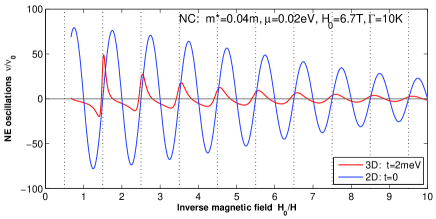
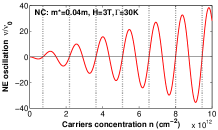
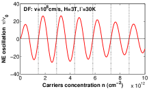
Figure 1: Normalized Nernst-Ettingshausen (NE) oscillation as function of the inverse magnetic field and carriers concentration for normal carriers (NC) and Dirac fermions (DF). Dependence $\nu(H^{-1})$ for DF has the same profile as for NC but shifted on half period. Vertical lines shows the quantization condition (1).

This equation can be inverted for $S(\mu):$

$$\frac{c}{e\hbar}\frac{S(\mu)}{2H}=\pi^{2}\frac{\hbar c}{e}\frac{n}{H}-\arctan\frac{\sin 2\pi\left(\pi\frac{\hbar c}{e}\frac{n}{H}-\gamma\right)}{e^{\frac{2\pi\Gamma}{\hbar\omega_{c}}}+\cos 2\pi\left(\pi\frac{\hbar c}{e}\frac{n}{H}-\gamma\right)}.$$ (17)

Equation (17) yields the dependence $\mu(n,H)$. Substituting it to Eq. (15) after some cumbersome algebra one can find the oscillating part of the Nernst coefficient explicitly:

$$\widetilde{\nu}^{\left(2D\right)}\left(n,H\right)=\frac{2\pi^{3}}{3}\frac{T}{\hbar\omega_{c}}\frac{\kappa\left(H\right)}{\sinh\frac{2\pi\Gamma}{\hbar\omega_{c}}}\sin 2\pi\left(\pi\frac{\hbar c}{e}\frac{n}{H}-\gamma\right),$$ (18)

that is a strongly oscillating function. It crosses zero at the intersections of LL and chemical potential, given by the condition $H=H_{k\sigma}$ defined by (1). The field depended factor $\kappa\left(H\right)$ is governed by magnetoresistance and is given by Eq.(13). At $\omega_{c}\tau\leq 1$ where SdH oscillations are small, $\kappa\left(H\right)$  can be roughly estimated using the Drude approximation (14). In particular, approaching the limit $\omega_{c}\tau\sim 1$ and assuming $\Gamma\sim\hbar/2\tau$ we obtain that $\kappa\left(H\right)\sim\frac{\tau}{m^{\ast}c}$ and the amplitude of NE oscillations is giant in comparison with the background: $\widetilde{\nu}^{\left(2D\right)}\sim\frac{\varepsilon_{F}}{\hbar\omega_{c}}\nu_{0}$. At higher fields $\omega_{c}\tau>1$, in the quantum Hall regime, the shape of oscillations of the NE coefficient is affected by strong variation of the magnetoresistance and Dingle temperature. This can be taken into account by substitution of the field dependent magnetoresistance and Dingle temperature into Eqs. (12),(13).

The given by Eq. (18) profiles of 2D NE oscillation as function of $H$ and $n$ for DF and NC are presented in Fig.1. Both our theory for DF and experiment in graphene 2009Zuev ; 2009Checkelsky show a $\sin$-like profile of the signal whose amplitude slightly decreases with increasing $n$. This tendency contradicts to the earlier theoretical predictions of the classical Mott formula 2009Zuev that has been derived for a Boltzmann gas of electrons. In contrast, the amplitude of NE oscillations increases with increasing $n$ for the NC in a qualitative agreement with the Mott formula.

Quasi-2D and 3D cases. In order to describe the NE effect in the general quasi-2D case where $t\neq 0$ the Bessel function in the Eq. (7) should be taken into account. The sums (9) can be reduced to the integrals by means of the Poisson transformation. Then integration can be done analytically resulting in

$$\Xi^{\left\{0\right\}}=\frac{1}{2}\sum_{\begin{subarray}{c}k=-\infty\\ \sigma=\pm 1\end{subarray}}^{\infty}\frac{1}{2\pi\left[\delta_{k\sigma}^{2}\left(H\right)+\frac{4t^{2}}{\hbar^{2}\omega_{c}^{2}}\right]^{1/2}}-\frac{1}{2},$$ (19)

$$\Xi^{\left\{1\right\}}=-\frac{1}{6}\frac{T}{\hbar\omega_{c}}\frac{1}{2}\sum_{\begin{subarray}{c}k=-\infty\\ \sigma=\pm 1\end{subarray}}^{\infty}\frac{\delta_{k\sigma}\left(H\right)}{\left[\delta_{k\sigma}^{2}\left(H\right)+\frac{4t^{2}}{\hbar^{2}\omega_{c}^{2}}\right]^{3/2}},$$ (20)

where $\delta_{k\sigma}\left(H\right)=\frac{\Gamma}{\hbar\omega_{c}}-i\frac{c}{\hbar e}\frac{S}{2\pi}\left(H^{-1}-H_{k\sigma}^{-1}\right)$. The NE coefficient is obtained by substitution of the Eqs. (19), and (20) to Eq. (12). Resonances at $i\delta_{k\sigma}\left(H\right)=\pm\frac{2t}{\hbar\omega_{c}}$ in $\widetilde{\nu}\left(H\right)$ appear when the chemical potential crosses the quantized slices of maximal (minimal) cross sections of the corrugated cylinder FS $S_{\max(\min)}=S\pm 4\pi tm^{\ast}$.

In the wide quasi 2D interval $t<\left(\hbar\omega_{c}\right)^{2}/\Gamma$ the behavior of $\widetilde{\nu}^{(q2D)}\left(H\right)$ close to $H=H_{k\sigma}$ can be studied selecting in (19) and (20) only the resonant terms. With growth of $t$ the positions of zeros shift from $\mathrm{Im}\delta_{k\sigma}\left(H\right)=0$ to $\mathrm{Im}\delta_{k\sigma}\left(H\right)=\pm\frac{2t}{\hbar\omega_{c}}$. The superposition of two (for $S_{\max}$ and $S_{\min}$) series of resonances leads to the beats in $\widetilde{\nu}\left(H\right)$ oscillations.

In the 3D limit $t>\left(\hbar\omega_{c}\right)^{2}/\Gamma$ , $\mathrm{Re}\Xi^{\left\{0\right\}}\ll 1$, so that $\Xi^{\left\{0\right\}}$ can be neglected in the denominator of Eq. (12). In the vicinity of $H=H_{k\sigma}$ one finds

$$\widetilde{\nu}^{(3D)}\left(H\right)=\mp\frac{\pi}{12}\frac{T\kappa\left(H\right)}{\left(t\hbar\omega_{c}\right)^{1/2}}\mathrm{Re\,}\frac{1}{\left[\frac{2t}{\hbar\omega_{c}}\pm i\delta_{k}\left(H\right)\right]^{3/2}},$$ (21)

We assumed here the constant $\mu$ and neglected Zeeman splitting, taking $\delta_{k,\pm 1}=\delta_{k}$. The resonances in $\widetilde{\nu}\left(H\right)$ described by Eq. (21) have the form of asymmetric spikes with $\left|\widetilde{\nu}^{(3D)}\right|_{\max}/\left|\widetilde{\nu}^{(3D)}\right|_{\min}\simeq 3.4$ as shown in Fig.1. In the Drude approximation, the amplitude

$$\left|\widetilde{\nu}^{(3D)}\right|_{\max}\simeq 0.29\frac{\varepsilon_{F}}{\Gamma}\frac{\hbar\omega_{c}}{\left(t\Gamma\right)^{1/2}}\nu_{0}\left(H\right)$$ (22)

is giant if $\frac{\varepsilon_{F}}{\Gamma}\frac{\hbar\omega_{c}}{\left(t\Gamma\right)^{1/2}}>1.$  

For 2D systems our calculations are valid for magnetic fields $\omega_{c}\lesssim\tau^{-1}$ where one can neglect the quantum Hall oscillations of conductivity. At higher fields the approach of Girvin and Jonson 1982Girvin , based on the generalized Mott formula for the thermopower tensor for 2D systems, seems to be more relevant. In 3D case the range of applicability of our theory is given by $\omega_{c}\ll\varepsilon_{F}$. Recently Bergman and Oganesyan 2010Bergman extended the approach of Ref. 1982Girvin to calculate the off-diagonal thermoelectric conductivity $\alpha_{xy}$ for a 3D system at $\omega_{c}\sim\varepsilon_{F}$. Although $\alpha_{xy}$ constitute only the part of the NE coefficient $\nu=-\left(\rho_{xx}\alpha_{xy}+\rho_{xy}\alpha_{yy}\right)/H$, they reproduce quite well the measured in graphite 2009Zhu sawtooth dependence of $\nu(H)$, having the characteristic $(H_{k}-H)^{-\frac{1}{2}}$ divergencies at resonances.

 In conclusion, we have obtained an analytical expression for the oscillating NE constant in a 2D system with an arbitrary electron dispersion, describing the recent experimental results in graphene and predicting a qualitative difference in the NE oscillations for NC and DF. We show that the giant oscillations of the NE coefficient predicted and observed in a 2D case (graphene) decrease significantly as the spectrum acquires a 3D character (graphite). We describe analytically the shape of NE oscillations. The NE oscillations are proportional to the temperature derivative of the dHvA oscillations.

This work was supported by FP7-IRSES programs: ROBOCON and SIMTECH.

References

• (1) A.Ettingshausen, W.Nernst, Wied. Ann. 29, 343 (1886).
• (2) K. Behnia , M-A. Méasson and Y. Kopelevich, Phys. Rev. Lett. 98, 076603 (2007)
• (3) E.H. Sondheimer, Proc. R. Soc. London 193, 484 (1948).
• (4) Yu.N. Obraztsov , Sov. Phys. Solid State  6, 331 (1964).
• (5) C.J. Bergeron, C.G. Grenier, and J.M.Reynolds, Phys. Rev. Lett. 2, 40 (1959).
• (6) I. M. Lifshitz and A. M. Kosevich, Zh. Éksp. Teor. Fiz. 29, 730 (1955).
• (7) Y. M. Zuev, W. Chang and P. Kim, Phys. Rev. Lett. 102, 096807 (2009)
• (8) J.G. Checkelsky, N.P. Ong, Phys. Rev. B 80, 081413(R) (2009)
• (9) D.L. Bergman and V. Oganesyan, Phys. Rev. Lett. 104, 066601 (2010)
• (10) K. Behnia , M-A. Méasson and Y. Kopelevich, Phys. Rev. Lett. 98, 166602 (2007)
• (11) Z.Zhu,H.Yang,B.Fauque et al. Nature Phys. 6, 26 (2009)
• (12) L. A. Falkovsky, Zh. Éksp. Teor. Fiz. 49, 609 (1965) [Sov. Phys. JETP 22, 609 (1966)]
• (13) G. P. Mikitik and Yu.V. Sharlai, Phys. Rev. Lett. 82, 2147 (1999).
• (14) M.N. Serbyn, M. A. Skvortsov, A. A. Varlamov, and V. Galitski , Phys. Rev. Lett. 102, 067001 (2009).
• (15) A.A. Varlamov and A.V. Kavokin, Europhys. Lett. 8 6, 47007 (2009).
• (16) T. Champel, V.P. Mineev, Philosophical Magazine B81, 55 (2001).
• (17) A. M. Bratkovsky and A. S. Alexandrov, Phys. Rev. B 65, 035418 (2002)
• (18) I. A. Luk’yanchuk and Y. Kopelevich, Phys. Rev. Lett. 93, 166402 (2004).
• (19) M. Jonson and S. Girvin, Phys. Rev. B29, 1939 (1984).