Two-dimensional Vesicle Dynamics under Shear Flow: Effect of Confinement

Abstract

Dynamics of a single vesicle under shear flow between two parallel plates is studied in two-dimensions using lattice-Boltzmann simulations. We first present how we adapted the lattice-Boltzmann method to simulate vesicle dynamics, using an approach known from the immersed boundary method. The fluid flow is computed on an Eulerian regular fixed mesh while the location of the vesicle membrane is tracked by a Lagrangian moving mesh. As benchmarking tests, the known vesicle equilibrium shapes in a fluid at rest are found and the dynamical behavior of a vesicle under simple shear flow is being reproduced. Further, we focus on investigating the effect of the confinement on the dynamics, a question that has received little attention so far. In particular, we study how the vesicle steady inclination angle in the tank-treading regime depends on the degree of confinement. The influence of the confinement on the effective viscosity of the composite fluid is also analyzed. At a given reduced volume (the swelling degree) of a vesicle we find that both the inclination angle, and the membrane tank-treading velocity decrease with increasing confinement. At sufficiently large degree of confinement the tank-treading velocity exhibits a non-monotonous dependence on the reduced volume and the effective viscosity shows a nonlinear behavior.

I Introduction

The study of blood flow at the microscale, i.e. the scale of blood corpuscules, is an important issue. In recent years this field has embraced several communities ranging from medical scientists to mathematicians. Classical continuum approaches of blood flow, dating back to a century ago at least Fung , are based on several assumptions and approximations that are both difficult to justify or to validate. For example, in the microvasculature, where most of the blood flow resistance takes place, red blood cells (RBCs), which are by far the major component of blood, have a size which is of the same order as that of the blood vessel diameter. Thus, one expects that the discrete nature of blood should play a decisive role in microcirculation. A prominent example is the Fahraeus–Lindqvist effect: RBCs cross-streamline migration towards the blood vessel center results in a dramatic collapse of blood viscosity, causing a reduction of blood flow resistance in the microvasculature. Even in larger blood vessels (e.g. veins, arteries) a satisfactory phenomenological continuum approach is lacking. One may thus hope that a constitutive law for blood will ultimately emerge from numerical simulations taking explicitly into account the blood elements. Still blood flow simulation is a challenging task since it requires solving for the dynamics of both the blood elements and the suspending fluid (plasma).

Different numerical methods have been developed to study RBCs or their bimimetic counterparts (represented by vesicles and capsules), each having its own advantages and drawbacks. A widely used method is the boundary integral method which is based on the use of Green’s function techniques Pozrikidis . It has been successfully applied to vesicles Kraus1996 ; Cantat1999 ; Biros2008 ; Biben2010 . The advantage of this method is the high precision. However, except for special geometries (e.g. unbounded fluid domain, semi-infinite domain), an appropriate Green’s function is not available. This means that extra integrations over boundaries delimiting the fluid have to be performed, which increases the computational time significantly. In addition, this method is valid for Stokes flow only (no inertia). Other classes of methods are phase-field Biben2003 ; Biben2005 ; Du2006 and level set approaches Maitre2010 which can be applied both in the Stokes and Navier-Stokes regimes. Their advantage is the ability of handling, in principle, many particles by just specifying the initial condition (in any new run with different vesicles number only specifying initial conditions is required in principle!). However, these methods introduce a finite thickness of the membrane, which seems, up to now, to set a quite severe limitation regarding extraction of quantitative data in the dynamical regimes. This requires a finite element technique with a grid refinement. Other types of methods consist of solving the fluid equations by adopting a ”coarse-grained or mesoscopic” technique. Examples include the so-called multiparticle collision dynamics (MPCD) or stochastic rotation dynamics (SRD) Malvanets1999 ; Noguchi2005 . Its advantages are the relative ease of implementation and inherent thermal fluctuations which make the method very efficient if these are required.

In this paper we apply an alternative mesoscopic method, namely the lattice-Boltzmann (LB) method. In the spirit of the LB method, a fluid is seen as a cluster of pseudo-fluid particles, that can collide with each other when they spread under the influence of external applied forces. Advantages of the LB method are its relative ease of implementation together with its versatile adaptability to quite arbitrary geometries. The LB method has been already adapted and used to perform simulations of deformable particles such as capsules Zhang2007 , vesicles and red blood cells Dupin2007 under flow. The main issue of the work presented in Dupin2007 is to accomplish simulations with a large number of particles while using a small number of nodes to reduce the computational time and the required memory. This has been achieved by using ad hoc membrane forces that penalize any deviation from the equilibrium configuration. In the present paper we use the precise analytical expression of the local membrane force as it has been derived Kaoui2008 from the known Helfrich bending energy Helfrich1973 . The perimeter conservation in our case is achieved by using a field of local Lagrangian multiplicators (equivalent to an effective tension). To accomplish the fluid-vesicle coupling we follow the same strategy used in Zhang2007 to simulate capsules dynamics. In Zhang2007 the flow is computed by LB. The flow-structure two-way coupling is achieved using the Immersed Boundary Method (IBM). Although confining walls were considered in the above mentioned studies their effect on the dynamics was not studied. We believe that it is of interest to study the impact of the walls on the dynamics of vesicles, a question that to the best of our knowledge has not been treated in the literature so far for vesicles, capsules or red blood cells, but only for a droplet Janssen2007 and a hard sphere Sangani2010 .

Vesicles are closed lipid membranes encapsulating a fluid and are suspended in an aqueous solution. Their membrane is constituted of lipid molecules (also the major component of the RBC membrane) Lipowsky1995 . Each one has a hydrophilic head and a two hydrophobic tails. These molecules re-organize themselves if they are in contact with an aqueous solution, or properly speaking self-assemble, into a bilayer in which all the heads of the molecules are facing either the internal fluid or the external one. Experimentally, vesicles with size of the order of $10\mu m$ - called Giant Unilamellar Vesicles (GUV) - can be easily prepared in the laboratory using, for example, the electro-formation technique Angelova1992 . Unlike RBCs, for vesicles we can vary their intrinsic characteristic parameters (size, degree of deflation, nature of internal fluid, etc…). Despite the simplicity of their structure, vesicles have exhibited many features observed for red blood cells: equilibrium shapes Seifert1991 , tank-treading motion Fischer1978 ; Kraus1996 , lateral migration Secomb2007 ; Kaoui2008 ; Coupier2008 , or slipper-like shapes Skalak1969 ; Kaoui2009a . Capsules (a model system incorporating shear elasticity) have also revealed some common features with vesicles Bagchi1 ; Bagchi2 .

In the following sections we briefly introduce the formulation of the LB method for vesicles. We then study in two-dimensions (2D) the tank-treading motion of a single vesicle under shear flow between two parallel plates. Here we decided for 2D simulations since they are computationally less demanding, but still capture all the relevant physics. We use large systems (in lattice units) because of the higher resolution required to extract the results shown below. Previous works done in 2D dealing with vesicles (also for red blood cells) have demonstrated that the dynamics in the third dimension is not relevant even in confined geometries Secomb2007 ; Coupier2008 ; Finken2008 . Vesicle dynamics under shear has been extensively studied in the literature. It is known that a vesicle placed in shear flow performs different kinds of motions depending on its degree of deflation, the viscosity contrast between the internal and the external fluids and on the strength of the shear flow (see the phase-diagram in Kaoui2009b ). When the viscosities of the internal and the external fluids are identical the vesicle performs a tank-treading motion. Its main long axis gets a steady inclination angle with respect to the flow direction while its membrane undergoes a tank-treading like motion. However, in the majority of the previous theoretical and numerical works the vesicle is placed in an infinite fluid (unbounded domain). This corresponds to the situation where the walls are too far from the vesicle to have any influence on its dynamics. For this reason here we study vesicle dynamics in a confined geometry. However, studying numerically the dynamics of vesicles in such conditions is a challenging problem from a computational point of view, especially in highly confined situations. We need to solve for the flow of the internal and the external fluids. The boundary separating the two fluids is also an unknown quantity since the membrane shape is not known a priori.

Since the vesicle size ($\sim 10\mu m$) is much larger than its membrane thickness ($\sim 5nm$), mathematically we model the membrane as an interface with zero thickness. Tracking the motion of this freely moving interface under flow is not a simple task, especially when the membrane undergoes larger deformations due to hydrodynamical stresses. We need to label the interface by points which we track in time. Further, to take into account the deformation an increased number of label points is required for the code to be stable and to capture deformation with good resolution. On the other hand, spatial derivatives on the membrane are needed to be evaluated at every time step to compute the membrane force. We need to evaluate the local curvature that is the fourth derivative of the vector position. Any formation of a highly buckled region in the membrane will introduce potential instability. Furthermore, the vesicle volume (the enclosed area in 2D) and its surface area (the perimeter in 2D) have to be kept conserved in time. At higher degrees of confinement possible undesirable contact between the membrane and the walls of the channel can be expected, and this is an additional difficulty to cope with. We do not use any ad hoc repulsive force from the wall, rather the non contact is achieved via a proper handling of the viscous lubrication forces by the lattice Boltzmann method.

We shall discuss how the vesicle-fluid coupling is accomplished. For that purpose an approach known from the immersed boundary method Mittal2005 is adopted. We present tests of the code by investigating vesicle equilibrium shapes in a fluid at rest. We then present simulation results regarding the steady inclination angle and the effective viscosity, as well as the tank-treading velocity as functions of the reduced volume and the degree of confinement.

II The lattice-Boltzmann method

The motion of the membrane can be induced by exerting an externally applied flow, and this is the physical situation we are interested in. In the present section we discuss how the fluid flow is solved for by using the LB method. In recent decades, the LB method has been introduced and widely used to simulate e.g. fluid flow in complex geometries (e.g. in porous media), multi-component and multi-phase flow (e.g droplets and binary fluids) Succi2001 ; Sukop2006 . Such popularity of the LB method among scientists and engineers has been gained thanks to its straightforward implementation and its local nature that allows for parallel programming.

In the limit of small Mach $Ma$ (ratio of the speed of a fluid particle in a medium to the speed of sound in that medium) and Knudsen $Kn$ (ratio of the molecular mean free path to the macroscopic characteristic length scale) numbers the LB method is known to recover with good approximation the Navier-Stokes equations Succi2001 ; Sukop2006 :

$$\rho\left(\frac{\partial\textbf{u}}{\partial t}+\textbf{u}\cdot\nabla\textbf{u}\right) = -\nabla p+\eta\nabla^{2}\textbf{u}+\textbf{F},$$ (1)

$$\nabla\cdot\textbf{u} = 0,$$ (2)

governing the fluid flow of an imcompressible Newtonian fluid. $\rho$ and $\eta$ are the mass density and the dynamic viscosity of the studied fluid, u and $p$ are its velocity and pressure fields, and $t$ is the time. F on the right-hand side is a bulk force (e.g. gravity) or the membrane forces as is the case for vesicles immersed in that fluid (see below). In the spirit of the LB method, a fluid is seen as a cluster of pseudo-fluid particles, that can collide with each other when they spread under the influence of external applied forces. In the LB context, not only the spatial position is discretized but also the velocity. This implies that every pseudo-fluid particle can move just along discrete directions with given discrete velocities. The main quantity associated with a pseudo-fluid particle is the distribution function $f_{\text{i}}(\textbf{r},t)$, with $0\leq f_{\text{i}}\leq 1$, which gives the probability of finding at time $t$ the pseudo-fluid particle at position r and having velocity $\textbf{c}_{\text{i}}$, in the $i$-direction. There is no unique way in the choice of a lattice in the LB method. What matters is that the discretization has to fulfill the following constraints: mass conservation, momentum conservation and isotropy of the fluid. Here, we adopt the so-called the D2Q9 lattice, where D2 is an abbreviation for two-dimensional space while Q9 refers to the number of possible discrete velocity vectors Qian1992 .

The evolution in time of the distribution $f_{\text{i}}$ is governed by the LB equation:

$$f_{\text{i}}(\textbf{r}+\textbf{c}_{\text{i}}\Delta t,t+\Delta t)-f_{\text{i}}(\textbf{r},t)=\Delta t\left(\Lambda_{\text{i}}+F_{\text{i}}\right)\quad(i=0...8),$$ (3)

where $f_{\text{i}}(\textbf{r},t)$ is the old distribution of the pseudo-fluid particle when it was at position r at previous time $t$, $f_{\text{i}}(\textbf{r}+\textbf{c}_{\text{i}}\Delta t,t+\Delta t)$ is the new distribution of the same pseudo-fluid particle after it moved in the direction $\textbf{c}_{\text{i}}$ to the new location $\textbf{r}+\textbf{c}_{\text{i}}\Delta t$ during the elapsed time $\Delta t$, with $\Delta t$ being the time step. The grid spacing is referred to by $\Delta x$. In this paper all units are given in lattice-units, where $\Delta x=\Delta t=1$. The left-hand side of Eq. (3) alone represents the free propagation of the pseudo-fluid particles without externally applied forces. In the right-hand side of Eq. (3), $F_{\text{i}}$ is any externally applied force and $\Lambda_{\text{i}}$ is the collision operator. Here, we adopt the Bhatnagar-Gross-Krook (BGK) approximation which is given by

$$\Lambda_{\text{i}}=-\frac{1}{\tau}\left[f_{\text{i}}(\textbf{r},t)-f_{\text{i}}^{\text{eq}}(\textbf{r},t)\right].$$ (4)

The BGK collision operator describes the relaxation of the distribution $f_{\text{i}}(\textbf{r},t)$ towards an equilibrium distribution $f_{\text{i}}^{\text{eq}}(\textbf{r},t)$, with a relaxation time $\tau$. This relaxation time is set to 1 in this paper and related to the dynamic viscosity $\eta$ via the relation:

$$\eta=\nu\rho=\rho c_{\text{s}}^{2}\frac{\Delta x^{2}}{\Delta t}\left(\tau-\frac{1}{2}\right),$$ (5)

where $c_{\text{s}}=1/\sqrt{3}$ is the speed of sound for the D2Q9 lattice. $f_{\text{i}}^{\text{eq}}(\textbf{r},t)$ is the equilibrium distribution obtained from an approximation of the Maxwell-Boltzmann distribution and is given by

$$f_{\text{i}}^{\text{eq}}(\textbf{r},t)\!=\!\omega_{\text{i}}\rho(\textbf{r},t)\!\left[\!1\!+\!\frac{1}{c_{s}^{2}}\left(\textbf{c}_{i}\!\cdot\!\textbf{u}\right)\!+\!\frac{1}{2c_{s}^{4}}\left(\textbf{c}_{\text{i}}\!\cdot\!\textbf{u}\right)^{2}\!-\!\frac{1}{c_{s}^{2}}\left(\textbf{u}\!\cdot\!\textbf{u}\right)\!\right]\!,$$ (6)

where $\omega_{\text{i}}$ are weight factors. $\omega_{\text{i}}$ equals $4/9$ for the $0$ velocity vector, $1/9$ in the horizontal and vertical directions and $1/36$ in the diagonal directions. The macroscopic quantities describing the flow are given by

$$\rho(\textbf{r},t)=\sum_{\text{i}=0}^{8}f_{\text{i}}(\textbf{r},t),$$ (7)

for the local mass density,

$$\textbf{u}(\textbf{r},t)=\frac{1}{\rho(\textbf{r},t)}\sum_{\text{i}=0}^{8}f_{\text{i}}(\textbf{r},t)\textbf{c}_{\text{i}},$$ (8)

for the local fluid velocity and

$$p(\textbf{r},t)=\rho(\textbf{r},t)c_{\text{s}}^{2},$$ (9)

is the local fluid pressure.

The computational domain is a rectangular box, with length $2L$ and height $2W$. We use $x$ for the horizontal position of the box and $y$ for the vertical position. Periodic boundary conditions are imposed on the right and on the left side of the box. To generate a shear flow, the upper and lower walls are displaced with the same velocity $\textbf{u}_{wall}$ but in opposite directions. To achieve this numerically, within the LB technique, the following bounce back boundary conditions are implemented on the two walls as Ladd1994

$$f_{-i}(\textbf{r},t+\Delta t)=f_{i}(\textbf{r},t)+2\frac{\rho w_{i}}{c_{s}^{2}}(\textbf{u}_{wall}\cdot\textbf{c}_{1}).$$ (10)

Here, $f_{-i}$ denotes the distribution function streaming in the opposite direction of $i$. In the absence of a vesicle, the flow relaxes towards a steady linear shear velocity profile of the form $\textbf{u}^{\infty}=\gamma y\textbf{c}_{1}$, where $\gamma=u_{wall}/W$ is the shear rate.

III Fluid-vesicle interaction

We denote by $\Omega_{\rm ext}$, $\Omega_{\rm int}$ the fluid domains outside and inside the vesicle, respectively, and by $\Gamma$ the vesicle boundary. The flow has to be computed considering boundary conditions on the membrane, which is a free moving interface. At the membrane $\Gamma$ we require the continuity of the flow velocity

$$\textbf{u}^{\text{ext}}(\textbf{r}_{\text{m}})=\textbf{u}^{\text{int}}(\textbf{r}_{\text{m}})=\textbf{v}(\textbf{r}_{\text{m}}),\quad\text{with}\quad\textbf{r}_{\text{m}}\in\Gamma.$$ (11)

The $ext$ and $int$ suffixes are for the external and the internal fluids, respectively. v is the velocity of any point $\textbf{r}_{m}$ belonging to the membrane. The continuity of the tangential velocities of the two fluids on each side of the membrane follows from the assumption of the no-slip boundary condition at the membrane. Continuity of the normal velocity is a consequence of mass conservation (integrating the incompressibility condition $\nabla\cdot\textbf{u}=0$ on a small volume straddling membrane and using the divergence theorem yields that condition). Continuity of the two fluid velocities with that of the membrane expresses the fact that the membrane is non permeable (normal component) and that we assume full adherence (tangential component) Cantat2003 . Force balance (in the absence of inertia) implies that the net force acting on a membrane element is zero:

$$\left(\sigma^{\text{ext}}(\textbf{r}_{\text{m}})-\sigma^{\text{int}}(\textbf{r}_{\text{m}})\right)\textbf{n}=-\overline{\textbf{f}}(\textbf{r}_{\text{m}}),\quad\!\!\text{with}\!\!\quad\textbf{r}_{\text{m}}\in\Gamma.\!$$ (12)

$\sigma$ is the hydrodynamical stress expressed by $\sigma_{ij}=\eta(\partial_{i}u_{j}+\partial_{j}u_{i})-p\delta_{ij}$ and n the unit vector normal to the membrane, pointing from the interior domain of the vesicle to the exterior one. $\overline{\textbf{f}}$ is the force exerted by the membrane on its surrounding fluid and its expression is given below. At sufficiently large distance from the vesicle membrane, the perturbation of the velocity field due to the membrane decays so that the fluid flow recovers its undisturbed pattern:

$$\textbf{u}^{\text{ext}}(\textbf{r})\underset{|\textbf{r}-\textbf{r}_{\text{m}}|\rightarrow\infty}{\longrightarrow}\textbf{u}^{\infty}(\textbf{r}),$$ (13)

where $\textbf{r}_{\text{m}}\in\Gamma$ and $\textbf{r}\in\Omega_{ext}$.

In what follows we show how these boundary conditions can be used to achieve the coupling between the fluid flow and the vesicle dynamics. In the present work the internal and the external fluid flows are computed by the LB technique. The velocity and the pressure fields are computed on an Eulerian regular fixed mesh, while the vesicle membrane is represented by a Lagrangian moving mesh immersed in the previous fluid mesh. The adopted method is the so-called immersed boundary method (IBM). This method was developed by Peskin to simulate blood flow in the heart Peskin1977 . It is an adequate method to simulate deformable structures in flow (fluid-structure interaction). For a review see for example Ref. Mittal2005 . Within the framework of this method an interface (separating two regions occupied by two distinct fluids) is discretized into points interconnected by elastic ’springs’ (as illustrated in Fig. 1 for the case of a vesicle).

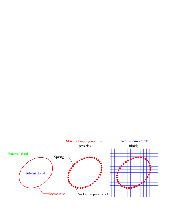
Figure 1: (Color online). Schematic view of a moving Lagrangian mesh representing a two-dimensional vesicle (where the membrane is represented by a contour) immersed in a fixed Eulerian mesh representing a fluid.

First, the fluid flow is computed in the whole computational domain by ignoring the existence of the interface. Then, the interface is advected by the actual fluid velocity, obtained from the Eulerian mesh by interpolation, as explained below. The fluid feels the existence of the vesicle due to singular point forces exerted by the interface nodes on their respective surrounding fluid nodes. This is achieved by linking the physical quantities computed on each mesh using a so-called discrete delta function suggested by Peskin Peskin2002 . The discrete delta function is defined as

$$\Delta(\mathbf{x})=\frac{1}{16\Delta x^{2}}\left(1+\cos\frac{\pi x}{\Delta x}\right)\left(1+\cos\frac{\pi y}{2\Delta x}\right)$$ (14)

for $|x|\leqslant 2\Delta x$ and $|y|\leqslant 2\Delta x$. In all other regions we set $\Delta(\mathbf{x})=0$, so that the function $\Delta$ has non zero values on a square. Here we choose $4\Delta x\times 4\Delta x$. The velocity at a given membrane node $\textbf{r}_{m}$ is evaluated by interpolating the velocities at its nearest fluid nodes $\textbf{r}_{m}$ using the above $\Delta$ function so that we obtain

$$\textbf{v}(\textbf{r}_{m})=\sum_{f}\Delta(\textbf{r}_{f}-\textbf{r}_{m})\textbf{u}(\textbf{r}_{f}).$$ (15)

Here, $\textbf{u}(\mathbf{r}_{f})$ is obtained from the LB procedure. Deducing the velocity on the membrane nodes from the velocity of the fluid nodes is possible since we consider that the fluid velocity is continuous across the membrane and that the vesicle points are massless, behaving as tracer-like particles, which do not disturb the flow at this stage. After evaluating every membrane node velocity we update its position using an Euler scheme

$$\textbf{r}_{m}(t+\Delta t)=\textbf{r}_{m}(t)+\textbf{v}(\textbf{r}_{m}(t)),$$ (16)

and consequently the vesicle is advected and deformed. However, the vesicle membrane is not a passive interface. It reacts back on the flow thanks to its restoring bending force

$$\overline{\mathbf{f}}({\mathbf{r}}_{m})\!=\!\left[\!\kappa_{B}\!\left(\frac{\partial^{2}H}{\partial s^{2}}+\frac{{H}^{3}}{2}\right)\!-\!H\zeta\right]\!\mathbf{n}+\frac{\partial\zeta}{\partial s}\mathbf{t}+\kappa_{A}\left(A\!-\!A_{0}\right)\mathbf{n},\!$$ (17)

where $H$ is the local membrane curvature, $\kappa_{B}$ is the bending modulus, $s$ is the arclength coordinate along the membrane (the contour in 2D), $\mathbf{n}$ and $\mathbf{t}$ are the normal and the tangential unit vectors, respectively. $\zeta$ is a Lagrange multiplier field that enforces local length conservation (the membrane is a one dimensional incompressible fluid). A detailed derivation of this force can be found in Kaoui2008 . The additional last term in Eq. (17) is introduced in order to enforce area conservation, because numerically a slight variation is observed (see Ref. Cantat2003 ). $A_{0}$ is the initial reference enclosed area of the vesicle, $A$ is its actual area and $\kappa_{A}$ a parameter that is chosen in a such a way to keep the vesicle area conserved. This conservation constraint can be improved also by increasing the resolution. The membrane force has non zero value only on the membrane and should vanish elsewhere. More precisely, a given fluid point $\textbf{r}_{f}$ is subject to the force

$${\bf F}({\textbf{r}_{f}})=\int_{\Gamma}{\overline{\mathbf{f}}(\textbf{r}_{m})}\delta({\textbf{r}_{f}-\textbf{r}_{m}})ds(\textbf{r}_{m}),\quad\text{with}\quad\textbf{r}_{m}\in\Gamma,$$ (18)

where $ds$ is the distance between two adjacent membrane points. However, since the membrane is discretized and thus presented by a cluster of points, this integral is rather a sum of the singular forces localized on the membrane nodes. In addition, writing the force felt by a fluid node in terms of an ordinary Dirac delta function is not adapted here, since the membrane nodes can be off-lattice and do not necessarily coincide with the fluid lattice nodes. The Dirac delta function in Eq. (18) is replaced by the $\Delta$ function suggested above which has a peak on the membrane node and decays at a distance equal to twice the lattice spacing after which it vanishes Peskin2002 . In this way the membrane force has a non zero value in a squared area of $4\Delta x\times 4\Delta x$ centered on the membrane node. The force then takes the form

$${\bf F}({\textbf{r}_{f}})=\sum_{m=1}^{n}{\overline{\mathbf{f}}(\textbf{r}_{m})}\Delta({\textbf{r}_{f}-\textbf{r}_{m}}).$$ (19)

Here, $n$ is the number of membrane nodes. The vesicle membrane finds itself, on the one hand, advected by its surrounding fluid and on the other hand it exerts a force in response to the applied hydrodynamical stresses, causing thereby a disturbance and modification of the fluid flow.

IV Simulation results and discussion

IV.1 Dimensionless numbers

The fluid flow and vesicle dynamics are controlled by the following dimensionless parameters:

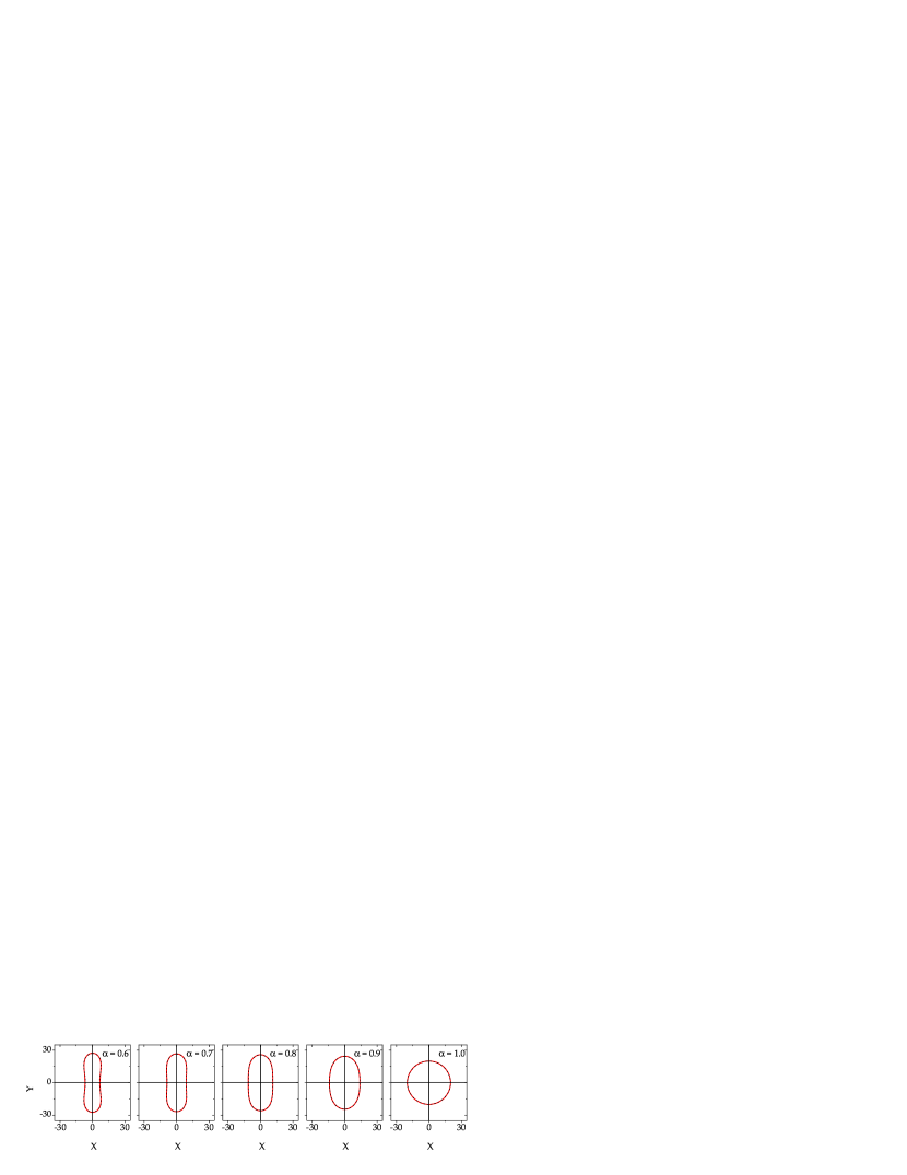
Figure 2: (Color online). Computed equilibrium shapes for vesicles having the same perimeter, but different reduced volumes $\alpha$. Red colored solid lines are shapes computed by the LB method. For comparison purpose and for validation, we plot also equilibrium shapes computed by the boundary integral method Beaucourt2004 (black dashed line).

• The Reynolds number

  $$\mbox{Re}=\frac{\rho\gamma R_{0}^{2}}{\eta},$$ (20)

  is associated to the applied shear flow and measures the importance of the inertial forces versus the viscous ones. $R_{0}$ is the effective vesicle radius. In 2D, $R_{0}$ can be deduced from the vesicle perimeter $R_{0}=P/2\pi$. In our simulations we use small enough values for Re (see below).

• The capillary number

  $$Ca=\frac{\eta\gamma R_{0}^{3}}{\kappa_{B}},$$ (21)

  represents the ratio between the shear time ($1/\gamma$) and the characteristic time ($\eta R_{0}^{3}/\kappa_{B}$) needed by a vesicle to relax towards its equilibrium shape after flow cessation. This parameter controls the deformability of the vesicle under flow. Larger $Ca$ lead to a larger deformability. Below we use the value $Ca=1$ which corresponds to the intermediate regime.

• The reduced volume (the swelling degree) quantifies how much a vesicle is swollen. In two dimensions it is given by

  $$\alpha=\frac{A}{A_{C}}=\frac{4\pi A}{P^{2}},$$ (22)

  where $A_{C}$ is the area of a circle having the same perimeter $P$ as the vesicle. $\alpha$ is unity for a circular vesicle (a maximally swollen vesicle) and less than unity for a deflated one $0<\alpha<1$.

• The viscosity ratio between the internal and external fluids is given by

  $$\lambda={\eta_{int}\over\eta_{ext}}.$$ (23)

  In this paper, however, this ratio is taken to be unity. For this value, a vesicle is expected to undergo tank-treading motion Keller1982 ; Kraus1996 ; Kantsler2005 .

• The tension number

  $$Ca_{s}=\frac{\eta\gamma R_{0}}{\kappa_{P}}$$ (24)

  is the ratio between the spring relaxation time (recall that $\kappa_{P}$ is the spring constant) and the shear time ($1/\gamma$). This number controls the inextensibility of the membrane under flow. To ensure the vesicle perimeter conservation constraint we set $Ca_{s}$ significantly small as compared to $Ca$ (below we set $Ca_{s}=1.05\times 10^{-5}$). For the simulations, we tune $\kappa_{P}$ until we get very negligible variations of the perimeter $P$. $\kappa_{P}$ is related to $\xi$ (the Lagrange multiplier) via the formula $\xi(s,t)=\kappa_{P}\left[ds(s,t)-ds(s,0)\right]$, where $ds(s,0)$ is the initial reference value Cantat2003 ; Kaoui2008 .

• The degree of confinement is given by the ratio of the vesicle’s effective radius to the channel half height,

  $$\chi=R_{0}/W.$$ (25)

IV.2 Computed equilibrium shapes

Finding the vesicle equilibrium shapes constitutes one of the benchmarking tests we use to validate our code. In contrast to a droplet, which adopts spontaneously a spherical equilibrium shape, vesicles can adopt different kinds of non-spherical shapes. In two-dimensions, a vesicle gets a circular equilibrium only for $\alpha=1$. Usually the equilibrium shapes are obtained by minimizing the Helfrich bending energy Helfrich1973

$$E=\frac{\kappa_{B}}{2}\int_{\Gamma}(2H)^{2}ds,$$ (26)

subject to the two constraints of vesicle area $A$ and perimeter $P$ conservation (in 2D). The only parameter controlling the shape of a vesicle, in the absence of an external applied flow and in unbounded domain, is its reduced volume $\alpha$ Seifert1991 . An alternative to energy minimization is to set the flow to zero ($Re=0$) and let the vesicle relax to its terminal shape. Technically, we place initially a vesicle with some shape (here an ellipse) in a fluid at rest (no shear flow). Then, the membrane starts to deform in order to relax towards the shape that minimizes its energy (Eq. 26). During this transition the membrane induces some weak fluid flow, inside and outside the vesicle. This flow stops once the vesicle gets its equilibrium shape. Figure 2 shows the computed equilibrium shapes for five vesicles having different values of the reduced volume $\alpha=0.6$, $0.7$, $0.8$, $0.9$, and $1$. The five vesicles have the same perimeter. Varying the reduced volume is achieved only by varying the vesicle area. It is somehow like swelling or deflating these vesicles to get different equilibrium shapes. To perform simulations we used the physical parameters $Re=Ca=0$ (fluid at rest), $R_{0}=20$ (to achieve a sufficient resolution at the scale of the LB grid) and $\chi=R_{0}/W=0.1$. We have set $n=100$, a value for which the code is stable. Significantly larger values of $n$ may cause instability. From this point of view, the LB method differs from the other conventional numerical schemes, for instance the boundary integral or the finite difference/element methods. In those methods, higher resolution and higher stability is achieved by increasing (without limit) the number of discretization points. In contrast, with the LB method an increase of $n$ induces higher resolution, but care should be taken not to exceed some given threshold value, beyond which the code destabilizes krueger-varnik-raabe:2010 . Therefore, in all our simulations we have kept a sufficiently small enough number of membrane nodes per lattice grid (by keeping the distance between two adjacent membrane nodes $ds$ close to $1$). Within the LB method the velocity has to be kept small enough (in our case we choose the limit of $0.1$) in order to have a sufficiently low Mach number and to ascertain the limit of neglectable fluid compressibility. The other parameters are chosen as follows. We have set $L=200$, so that the flow perturbation due to the presence of the vesicle is negligible at the computational domain boundaries where periodic boundary conditions are imposed. $\kappa_{A}=0.01$ to fulfil a precise enough conservation of the vesicle enclosed area (we measure a variation of the order of $0.00015\%$) and we set $\kappa_{P}=12$ to keep the perimeter conserved as well (variation of $0.00125\%$ is measured). The obtained shape for every given reduced volume is compared with its corresponding shape obtained by the boundary integral method, the black dashed lines in Fig. 2 (the same method as used in Refs. Kraus1996 ; Cantat1999 ; Beaucourt2004 ; Biros2008 ). For a given reduced volume, the computed equilibrium shapes obtained by both numerical methods are indistinguishable, especially at higher values of the reduced volume. In Fig. 2 we can see that for a reduced volume of $0.6$, the vesicle assumes a biconcave shape, as it is typical for healthy red blood cells.

IV.3 Tank-treading under shear flow

In the present section, we treat the effect of confinement on the dynamics of a tank-treading vesicle. First we study how the physical quantities, associated to the tank-treading regime, vary with the reduced volume. Then, for a given reduced volume, we analyze the effect of confinement on dynamics and rheology. We consider a single vesicle placed in a fluid subject to a simple shear. Here, we set $R_{0}=30$ in order to achieve a high enough resolution. For $R_{0}=30$, our explorations led us to the conclusion that $n=150$ is a good compromise between numerical stability and resolution. For this value of $n$ the code is stable even at higher degree of confinement. This also allows us to keep a sufficient number of fluid nodes between the wall and the membrane, a precision required in more confined situations. The length of the simulation box is set to $L=600$, chosen as to minimize perturbations by the vesicle at the edge of the simulation box, where periodic boundary conditions are imposed. Under such conditions and in the absence of a viscosity contrast ($\lambda=1$) a vesicle performs a tank-treading motion Keller1982 ; Kraus1996 ; Kantsler2005 . It deforms until reaching a steady fixed shape with its main axis assuming a steady inclination angle with respect to the flow direction. The membrane undergoes a tank-treading like motion and so it generates a rotational flow of the internal enclosed fluid.

IV.4 Effect of the reduced volume

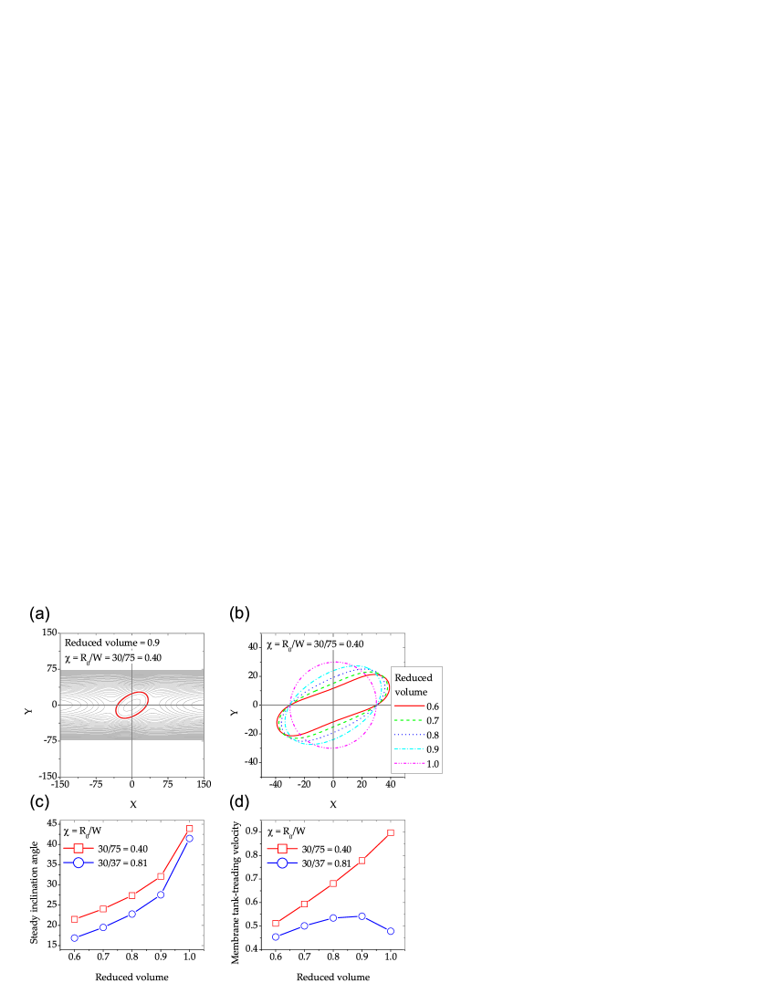
Figure 3: (Color online). Physical quantities associated to the tank-treading motion of vesicles (with $R_{0}=30$) under shear flow (with $Re=9.45\times 10^{-2}$ and $Ca=1$) in a confined channel: (a) streamlines pattern inside and outside a vesicle ($\alpha=0.9$) performing a tank-treading motion in a confined channel, (b) steady shapes for different values of the reduced volumes, (c) inclination angle versus the vesicle reduced volume for two degrees of confinement $\chi=R_{0}/W=0.40$ and $0.81$, (d) membrane tank-treading velocity (scaled by $\gamma R_{0}/2$, the rotational velocity of a circular vesicle under shear flow in unbounded geometry) versus the reduced volume.

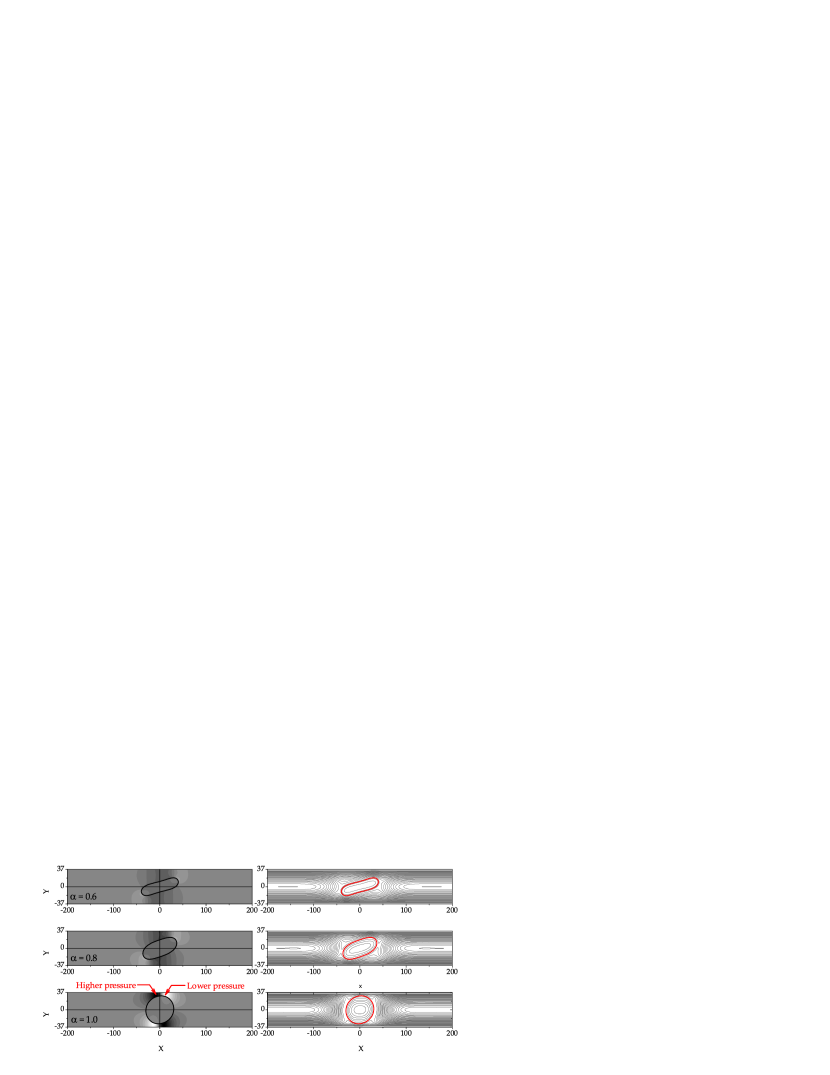
Figure 4: (Color online). Induced pressure field (with the grey scale) and flow streamlines (the gray solid lines in the right figure), inside and outside the vesicle, for different values of the reduced volume $\alpha=0.6$, $0.8$ and $1$. $Re=9.45\times 10^{-2}$, $Ca=1$ and $\chi=0.81$. The black solid lines in the left figures and the red solid lines in the right figures represent the vesicle membrane. In the right figures, the regions with black color correspond to higher pressure while the white regions correspond to lower pressure.

Figure 3 shows different physical quantities measured in the tank-treading regime. In Fig. 3a we show a vesicle performing tank-treading motion in a confined channel. The vesicle assumes a steady inclination angle (the red solid line). The streamlines inside and outside the vesicle (the gray solid lines) show that the internal fluid undergoes a rotational flow, induced by the membrane tank-treading. The external fluid exhibits recirculations at the rear (the left side of the figure) and at the front (the right side of the figure) of the vesicle. Such recirculations do not take place in the unbounded geometry Biros2008 . For a tank-treading vesicle in unbounded geometry (or at a sufficiently weak confinement), the external fluid lines are curved around the vesicle without being separated. In Fig. 3a the external fluid lines are separated into two portions before approaching the vesicle at two saddle points (located close to the channel centerline at the back and at the front of the vesicle): one portion continues its flow (through the region between the wall and the membrane) and passes the vesicle, while the other portion is reflected back by the vesicle. Such flow recirculations are also observed for confined rotating rigid spheres Wilson2005 and rigid ellipsoids Aidun2000 . For the same degree of confinement ($\chi=0.4$), in Fig. 3b we varied the reduced volume of the vesicle. In Fig. 3b we report the steady state shapes obtained for different values of the vesicle reduced volume. All the vesicles in Fig. 3b have been initialized with a zero inclination angle. Figure 3c shows the steady inclination angle as a function of the reduced volume (for two confinements: $\chi=0.4$ and $0.81$). The steady inclination angle increases monotonically (for both values of $\chi$) with increasing the reduced volume, until approaching $45$ degrees in the limiting case of circular vesicles. The same qualitative tendency is observed in the unbounded geometry Keller1982 ; Kraus1996 ; Beaucourt2004 .

Figure  3d shows the behavior of the tank-treading velocity normalized by $\gamma R_{0}/2$, which is the tank-treading velocity of a circular vesicle Ghigliotti2009 . For $\chi=0.4$, the tank-treading velocity increases monotonically with increasing the reduced volume, as observed for the unbounded geometry Keller1982 ; Kraus1996 ; Beaucourt2004 . However, for higher confinement, for example $\chi=0.81$, the tank-treading velocity does not vary anymore in a monotonous way. It has a maximum around $\alpha=0.85$ before it decreases at larger $\alpha$. This behavior can be explained by the fact that at higher degree of confinement, the amount of the external fluid which is able to flow from one side (the left) to the other side (the right) of the channel by crossing the narrow region between the wall and the membrane becomes smaller and smaller when increasing the reduced volume. At higher reduced volumes the inclination angle increases and so the membrane comes in closer proximity of the wall, see Fig. 4. Therefore, the external fluid flow does not participate fully to generate the tank-treading motion of the vesicle. This is also corroborated by the fact that the external fluid undergoes recirculation (see Fig. 3b and 4) meaning that part of the fluid is reflected backwards when approaching the vesicle. For a circular vesicle ($\alpha=1$) the amount of the reflected fluid is larger compared to the amount crossing the narrower region between the membrane and the walls.

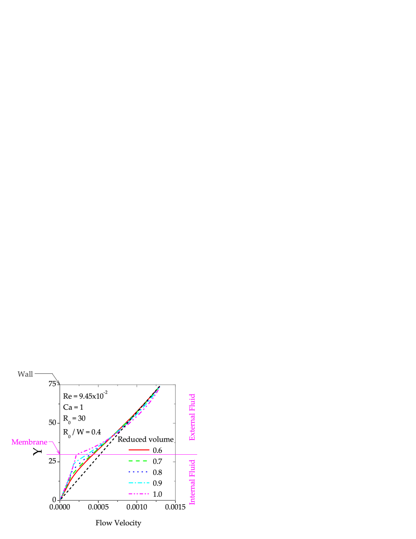
Figure 5: (Color online). Disturbed flow velocity profile measured at $x=0$ for different values of the vesicle reduced volume. The black dashed line is the undisturbed applied shear flow profile $u_{x}=\gamma y$ in the absence of the vesicle. The pink solid line corresponds to the location of the membrane for $\alpha=1$.

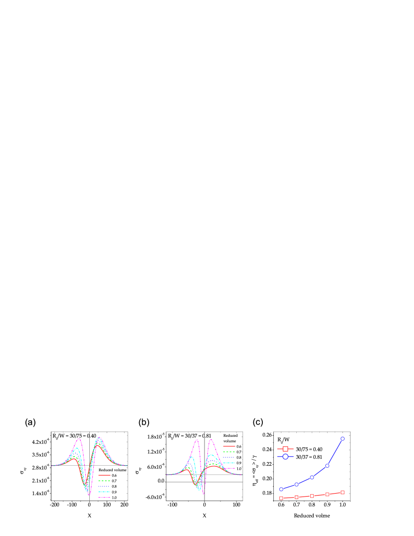
Figure 6: (Color online). The hydrodynamical stress exerted by the suspending fluid upon the bottom wall for two degrees of confinement, $\chi=0.4$ (a) and $0.81$ (b). The grey solid line is the stress calcuted analytically in the absence of the vesicle $\eta\gamma$. (c) The deduced effective viscosity of the fluid, in the presence of the vesicle, for both degrees of confinement.

The induced pressure field shown in the three left panels in Fig. 4 is significantly affected by increasing $\alpha$. For $\alpha=1$, a significant pressure gradient is observed at the inlet and the outlet of the narrower gap between the membrane and the wall. Such pressure drop along this narrower region generates an almost parabolic velocity profile, for the case of $\alpha=1$, as is shown in Fig. 5. In the same figure, for comparison purpose, we report the disturbed velocity profile for other different values of the reduced volume (these profiles are taken at $x=0$). The disturbance is maximal for $\alpha=1$.

The bounce back boundary condition of Ladd Ladd1994 allows to measure directly the hydrodynamical stress field $\sigma_{xy}$ exerted by the fluid upon the channel walls. Figures 6a and 6b show the measured hydrodynamical stress for two degrees of confinement, $\chi=0.4$ and $0.81$. The effective viscosity $\eta_{\rm eff}$ can be extracted from the hydrodynamical stress using the formula

$$\eta_{\rm eff}=\frac{\langle\sigma_{xy}\rangle}{\gamma},$$ (27)

where $\langle\sigma_{xy}\rangle$ refers to the volume average of the stress tensor. The stress $\sigma_{xy}$ has been averaged along the bottom wall. As shown in Figs. 6a and 6b the hydrodynamical stress on the bottom wall exhibits important variations for a larger reduced volume $\alpha$. For $\alpha=1$, the stress is symmetrical with respect to the vertical axis at $x=0$ (which is perpendicular to the walls and passing through the center of mass of the vesicle). This symmetry is also observed for confined rigid spheres Sangani2010 , and is a consequence of the symmetry of the Stokes equations upon time reversal. Actually, our simulation contains a small amount of inertia, but so small that the asymmetry is difficult to identify on the figure. For deflated vesicles ($\alpha\neq 1$) the stress curve has two unequal maxima and one minimum. The flow deforms the vesicle and breaks the up-stream/down-stream symmetry (see Fig. 4 for $\alpha=0.6$ and $\alpha=0.8$). In other words, the Stokes reversibility is broken by the shape deformation. The values of these maxima and minimum significantly deviate from the corresponding value $\eta\gamma$ in the absence of the vesicle (presented by the horizontal grey solid line in Fig. 6) upon increasing the reduced volume. By comparing Figs. 6a and 6b, one notices that the stress is important for higher degrees of confinement, as expected. Surprisingly, at higher $R_{0}/W$ we observe regions with negative hydrodynamical stress. We believe that this results from a subtle effect due to fluid recirculation around the vesicle. However, a clear explanation of this phenomenon is at present not available.

Figure 6c shows the behavior of the effective viscosity for different values of the vesicle reduced volume. The viscosity increases when increasing the reduced volume. The same tendency was observed for a vesicle placed in unbounded domain Ghigliotti2009 . This result is explained as follows: for a given confinement, the increase of the reduced volume implies a larger cross section of the vesicle in the channel (because of the large increase in the inclination angle), and this opposes more resistance to the fluid flow.

IV.5 Effect of confinement

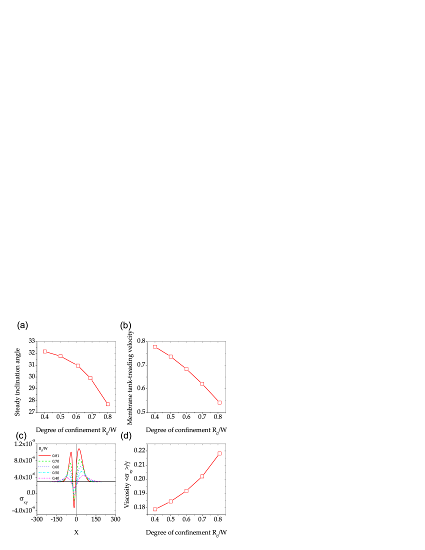
Figure 7: (Color online). Variation of the measured physical quantities associated to a vesicle performing tank-treading motion in confined geometries when varying the degree of confinement. (a) steady inclination angle, (b) the membrane tank-treading velocity (scaled by $\gamma R_{0}/2$), (c) the hydrodynamical stress field applied on the bottom wall and (d) the effective viscosity. Parameters are $\alpha=0.9$, $R_{0}=30$, $Re=9.45\times 10^{-2}$ and $Ca=1$.

Here we set ($\alpha=0.9$) and vary only the width ($2W$) of the channel in order to study the effect of confinement. All the other physical and numerical parameters are kept identical to those of the previous section. All simulations in Fig. 7 are performed with $\chi$ varying from $0.4$ to $0.81$. For this set of parameters, the code is still stable and guarantees a quite satisfactory conservation of the vesicle area and perimeter ($\Delta A/A_{0}\sim 0.00015\%$ and $\Delta P/P_{0}\sim 0.013\%$). Note that in Figure 7 we have kept the same shear rate $\gamma=1.75\times 10^{-5}$. Figure 7a shows a decrease of the inclination angle upon increasing confinement. Under confinement the angle saturates at smaller values as compared to the corresponding one in the unbounded flow. The wall acts via a hydrodynamical repulsive force (a viscous force) tending to push, so to speak, the orientation angle back to zero in order to align the vesicle with the flow. Such a decrease of the inclination angle was also reported by Janssen and Anderson Janssen2007 for a confined droplet under shear flow.

By decreasing confinement further, we expect to reach the unbounded geometry limit ($\chi=0$). We did not attempt to study this asymptotic limit. For $\chi<0.4$ and within the present resolution ($R_{0}=30$) a significant increase of $L$ is required in order to avoid unphysical effects induced by the periodic boundary conditions. This task requires a very high amount of computational time.

Figure 7b shows a decrease of the membrane tank-treading velocity (scaled by $\gamma R_{0}/2$) versus confinement. At high enough confinement, the external fluid does not anymore participate wholly in membrane tank-treading. The fluid is partially reflected backwards when approaching the vesicle, an effect that increases with confinement (see Fig. 8).

Figure 8: (Color online). Induced pressure field and flow streamlines, indside and outside the vesicle, for different values of the degree of confinement $\chi=0.81$, $0.6$ and $0.4$. Parameters are $\alpha=0.9$, $R_{0}=30$, $Re=9.45\times 10^{-2}$ and $Ca=1$.

For rigid spheres a similar decrease of the rotation velocity is also observed when increasing confinement Sangani2010 . Varying confinement affects also the way the membrane and the wall interact. Figure 7c shows the hydrodynamical stress exerted by the fluid on the bottom wall. The horizonal black solid line is the stress measured in the absence of the vesicle ($\eta\gamma$). At distances far from the location of the vesicle (on the extreme right and left sides of the figure) the stress measured for all degrees of confinement matches with the stress in the absence of the vesicle. In the vicinity of the vesicle, around $x=0$, we see deviation of the stress from the value $\eta\gamma$. Such deviations become larger and larger when increasing confinement. Again, as in the previous section, we observe stress with negative values at higher confinement. The effective viscosity is extracted from the stress (using Eq. 27) and the results are shown in Fig. 7d. The effective viscosity is found to significantly increase non-linearly with confinement.

In order to gain further insight we represent the pressure field and the streamlines (Fig. 8), for three different confinements, $\chi=0.81$, $0.6$ and $0.4$. Confining further the vesicle results in an increase of the pressure inside the vesicle, entailing a higher pressure gradient along the fluid layer located between the membrane and the wall. The amount of the fluid crossing this region decreases also when increasing confinement. The streamlines pattern shows that the recirculation becomes important at higher degree of confinement. Their two focal points move closer and closer to the vesicle when increasing confinement. A closer inspection of the pressure field and the streamlines (for a given degree of confinement $\chi$) reveals interesting dynamics occurring in the narrow region between the vesicle and the wall. When the external fluid approaches the vesicle it splits into two parts. One part is reflected by the vesicle and pushed backward without passing the vesicle. The other part continues its flow and crosses the narrower gap formed between the wall and the membrane. At the inlet, of this gap, the pressure is significantly higher, resulting in a slowing down of the fluid (the streamlines are separated). Once the fluid enters this region its velocity is amplified (the streamlines come closer), under the action of the pressure gradient along the gap, until it exits that region. At the outlet, the pressure drops to a lower value and the fluid is slowed down again (the streamlines separate again).

Finally, some general comments are worth mentioning. The fluid motion in the narrower gap, formed between the vesicle membrane and the wall, is induced under the action of three mechanisms: 1 - the membrane force, 2 - the shear flow and 3 - the pressure-gradient along this region. The third mechanism dominates at high confinement. In that regime the fluid (in the gap) is subject to the sum of forces induced by the above three mechanisms. Within the present method, this sum must not exceed some given threshold otherwise the code becomes unstable (due to higher flow velocities). There is also another technical detail that becomes problematic in situations of higher degrees of confinement. We assumed that the membrane has a zero thickness. However, by using the expression Eq. 14 the membrane force is distributed on fluid nodes located at distances of roughly $4\Delta x$ from the membrane. The membrane acquires a non-zero effective thickness. In more confined situations we need to leave at least $4$ fluid nodes in the gap between the membrane and the wall, otherwise the dynamics of the vesicle suffer from numerical artifacts. For example, a leakage of the internal fluid is observed, and the tank-treading velocity exhibited a non uniform behavior along the membrane. To overcome all these problems we had to increase the resolution. For the resolution of $R_{0}=30$ used in this section, the upper limit of the confinement we were able to reproduce without any apparent problem is $\chi=0.81$.

V Conclusion

We have studied the effect of confinement between two parallel walls on vesicle dynamics under shear flow. We limited ourselves to the case of having the same fluid inside and outside the vesicle. In such a situation the vesicle performs tank-treading motion. We developed a lattice-Boltzmann method to perform two-dimensional simulations. The coupling between fluid flow and vesicle dynamics was adopted from the immersed boundary method. Unlike previous works, we have introduced the membrane force by using its analytical expression as a function of the mean curvature and its derivative. The vesicle enclosed area and its perimeter are kept conserved in our method. We first computed the known vesicle equilibrium shapes for different values of the swelling degree in order to validate our code. The obtained shapes match perfectly the ones computed by the boundary integral method. As a second step, we studied the case of a vesicle placed in a domain bounded by two parallel walls. We induced the shear flow by moving these two walls in opposite directions. We found that both the vesicle inclination angle, with respect to the flow, and its membrane tank-treading velocity decrease when increasing the degree of confinement. Moreover, since at sufficiently large degree of confinement the vesicle membrane comes close to the wall so that just a very narrow region is left for the external fluid to flow. Therefore, the vesicle acts as an obstacle and thus the effective viscosity increases dramatically when increasing confinement. At a given degree of confinement, we varied the swelling degree. We observed the same qualitative tendency as for the unbounded geometry for the behavior of the angle, tank-treading velocity and viscosity as a function of the swelling degree. However at higher degree of confinement even the angle still shows an increase with increasing the swelling degree, the measured values are lower. The tank-treading velocity does not increase monotonically with the swelling degree. It exhibits a maximum value before getting to lower values in the limit of circular vesicles.

References

- (1) Y. C. Fung, Biomechanics (Springer, New York, 1990).
- (2) C. Pozrikidis, Boundary integral and singularity methods for linearized viscous flow, Cambridge University Press (1992).
- (3) M. Kraus, W. Wintz, U. Seifert, and R. Lipowsky, Phys. Rev. Lett. 77, 3685 (1996).
- (4) I. Cantat and C. Misbah, Phys. Rev. Lett. 83, 235 (1999).
- (5) S. K. Veerapaneni, D. Gueyffier, D. Zorin, and G. Biros, J. Comp. Phys. 228(7), 2334 (2009).
- (6) T. Biben, A. Farutin, and C. Misbah, arXiv:0912.4702v1.
- (7) T. Biben and C. Misbah, Phys. Rev. E 67 (2003).
- (8) T. Biben, K. Kassner, and C. Misbah, Phys. Rev. E 72 041921 (2005);
- (9) Q. Du, C. Liu, and X. Wang, J. Comp. Phys. 212, 757 (2006).
- (10) E. Maitre, C. Misbah, P. Peyla, and A. Raoult, preprint (2010).
- (11) A. Malevanets and R. Kapral, J. Chem. Phys. 110, 8605 (1999).
- (12) H. Noguchi and G. Gompper, PNAS 102(40), 14159 (2005)
- (13) R. Finken, A. Lamura, U. Seifert, and G. Gompper, Two-dimensional fluctuating vesicles in linear shear flow. Eur. Phys. J. E 25, 309 (2008)
- (14) J. Zhang, P. C. Johnson and A. S. Popel, Phys. Biol. 4, 285 (2007).
- (15) M.M. Dupin, I. Halliday, C.M. Care, and L.L. Munn, Phys. Rev. E 75 066707 (2007).
- (16) B. Kaoui, G.H. Ristow, I. Cantat, C. Misbah, and W. Zimmermann, Phys. Rev. E 77, 021903 (2008).
- (17) W. Helfrich, Z. Naturforsch. A 28c, 693 (1973).
- (18) R. Lipowsky and E. Sackmann, Structure and Dynamics of Membranes, from Cells to Vesicles (North-Holland, Amsterdam, 1995)
- (19) M. I. Angelova, S. Soléau, P. Méléard, J.-F. Faucon, P. Bothorel, Prog. Colloid Polym. Sci. 89, 127 (1992)
- (20) U. Seifert, K. Berndl, and R. Lipowsky, Phy. Rev. A 44, 1182 (1991)
- (21) T. M. Fischer, M. Stohr-Liesen, and H. Schmid-Schonbein, Science 24, 894 (1978)
- (22) G. Coupier, B. Kaoui, T. Podgorski and C. Misbah, Phys. Fluids 20, 111702 (2008)
- (23) T. W. Secomb, B. Styp-Rekowska, and A. R. Pries, Ann. Biomed. Eng. 35,755 (2007)
- (24) R. Skalak and P. I. Branemark, Science 164 717 (1969).
- (25) B. Kaoui, G. Biros, and C. Misbah, Phys. Rev. Lett. 103 188101 (2009)
- (26) S.K. Doddi, and P. Bagchi. Inter. J. Multiphase Flow 36, 966 (2008).
- (27) P. Bagchi and R. M. Kalluri, Phys. Rev. E 80, 016307 (2009).
- (28) B. Kaoui, A. Farutin, and C. Misbah, Phys. Rev. E 80, 061905 (2009)
- (29) R. Mittal and G. Iaccarino, Annu. Rev. Fluid Mech. 37, 239 (2005)
- (30) S. Succi, The Lattice Boltzmann equation (Oxford University Press, 2001)
- (31) M.C. Sukop, D.T. Thorne, Lattice Boltzmann modeling: an introduction for geoscientists and engineers (Springer, 2006)
- (32) Y. H. Qian, D. d’Humières, and P. Lallemand, Europhys. Lett. 17, 479 (1992)
- (33) A. J. C. Ladd, J. Fluid Mech. 271, 285 (1994)
- (34) I. Cantat, K. Kassner, and C. Misbah, Eur. Phys. J. E 10, 175189 (2003)
- (35) C. S. Peskin, J. Comput. Phys. 25, 220 (1977)
- (36) C. S. Peskin, Acta Numerica 11, 479 (2002)
- (37) S. R. Keller and R. Skalak, J. Fluid Mech. 120 (1982)
- (38) V. Kantsler and V. Steinberg, Phys. Rev. Lett. 95, 258101 (2005)
- (39) T. Krüger, F. Varnik, and D. Raabe, Comp. Math. Appl., in press (2010)
- (40) J. Beaucourt, F. Rioual, T. Séon, T. Biben, and C. Misbah, Phys. Rev. E 69, 011906 (2004)
- (41) M. C. T. Wilson and P. H. Gaskell, and M. D. Savage, Phys. Fluids 17, 093601 (2005)
- (42) E-J. Ding and C. K. Aidun, J. Fluid Mech. 423 (2000) 317
- (43) A. S. Sangani, A. Acrivos, L. Jibuti, and P. Peyla, (unpublished)
- (44) G. Ghigliotti, H. Selmi, B. Kaoui, G. Biros, and C. Misbah, ESAIM: PROC 28, 211 (2009)
- (45) P. J. A. Janssen and P. D. Anderson, Phys. Fluids 19, 043602 (2007)