A Selection Region Based Routing Protocol for Random Mobile ad hoc Networks with Directional Antennas

Abstract

In this paper, we propose a selection region based multihop routing protocol with directional antennas for wireless mobile ad hoc networks, where the selection region is defined by two parameters: a reference distance and the beamwidth of the directional antenna. At each hop, we choose the nearest node to the transmitter within the selection region as the next hop relay. By maximizing the expected density of progress, we present an upper bound for the optimum reference distance and derive the relationship between the optimum reference distance and the optimum transmission probability. Compared with the results with routing strategy using omnidirectional antennas in [1], we find interestingly that the optimum transmission probability is a constant independent of the beamwidth, the expected density of progress with the new routing strategy is increased significantly, and the computational complexity involved in the relay selection is also greatly reduced.

I Introduction

Determining the capacity region of wireless networks has been an open problem for more than half a decade. In the seminal work [2], Gupta and Kumar proved that the transport capacity for wireless ad hoc networks, defined as the bit-meters pumped every second over a unit area of the network, scales as $\Theta(\sqrt{n})$ in an arbitrary network, where $n$ is node density. In [3], Weber et al. derived the upper and lower bounds on the transmission capacity of spread-spectrum wireless ad hoc networks, where the transmission capacity is defined as the product between the maximum density of successful transmissions and the corresponding data rate, under a constraint on the outage probability. All these works address the single hop transmission. Recently, Baccelli et al. [4] proposed a spatial reuse based multihop routing protocol, and derived the optimum transmission probability. In their protocol, at each hop the transmitter selects the best relay to maximize the spatial density of progress. By assuming each transmitter has a sufficient backlog of packets, Weber et al. in [5] proposed the longest-edge based routing protocol where each transmitter selects a relay that makes the transmission edge longest. In [6], Andrews et al. defined the random access transport capacity with the maximum allowable total number of transmissions per packet along multiple hops. In [1], Li et al. proposed a selection region based multihop routing protocol to guarantee the message transmitted towards the final destination, where the selection region is defined by two parameters: a selection angle and a reference distance. By maximizing the expected density of progress, the author derived an upper bound on the optimum reference distance, and the relationship between the optimum reference distance and the optimum selection angle.

The above literatures only considered the wireless networks with omnidirectional antennas. In [7], Yi et al. investigated the wireless networks’ capacity using directional antennas, extending the network capacity with omnidirectional antennas in [2] to that with directional antennas. In [8], Spyropoulos et al. discussed the network capacity gain one can achieve by using directional antennas over that by using omnidirectional antennas and how these bounds are affected by important antenna parameters like gain and beamwidth. In [9], Dai et al. combined the multiple channels and directional antennas together and shown that they improve the network capacity due to the increased network connectivity and reduced interference. However, previous literature usually focuses on the scaling laws of the network capacity.

In this paper, we extend the former work in [1] with omnidirectional antennas to that with directional antennas, and derive the close-formed expected density of progress of the network, which is defined as the number of packets progress toward their destinations in a unit area of the network. Compared with the routing strategy using omnidirectional antennas in [1], due to the directional antennas, the selection region based routing is implemented much easier and the calculation burden for nodes to select the relay is also decreased.

The rest of the paper is organized as follows. Directional antenna model, network model and routing strategy are described in Section II. The optimization for selection region and transmission probability are presented in Section III. Numerical results and interpretations are given in Section IV. Finally, Section V summarizes our conclusions.

II Network Model and Routing Protocol

In this section, we first present the simplified directional antenna model, then define the network model and the selection region based routing protocol using directional antennas.

II-A Directional Antenna Model

In the study of wireless networks, the antenna model is often grouped into omnidirectional and directional. Omnidirectional antenna radiates signals equally well in all directions, while directional antenna has gain in the direction of the main lobe at which it is pointing. Thus, with directional antennas the interference can be decreased and nodes located in each other s neighborhood may transmit simultaneously, which increase spatial reuse of the channel. To simplify the analysis, we model the power pattern of the directional antenna as a circular sector with angle $\varphi$, where $\varphi$ is the beamwidth of the antenna, see Fig. 1. In the following analysis, we assume the transmitters with directional antenna and the receivers with omnidirectional antenna, which is called Directional Transmission and Omnidirectional Reception (DTOR) as mentioned in [7].

II-B Network Model

Assume nodes in the network follow a homogenous Poisson Point Process (PPP) with density $\lambda$, and slotted ALOHA as the medium access control (MAC) protocol. During each time slot a node chooses to transmit data with probability $p$, and to receive with probability $1-p$. Therefore, at a certain time instant, the transmitters follow a homogeneous PPP ($\Pi_{Tx}$) with density $p\lambda$, while the receivers follow another homogenous PPP ($\Pi_{Rx}$) with density $(1-p)\lambda$. At each hop in the multihop transmissions, a transmitter tries to find a receiver in $\Pi_{Rx}$ as relay. We consider the nodes are mobile, to eliminate the spatial correlation, which is also discussed in [4]. We also assume that all transmitters use a fixed transmission power $\rho$ and the wireless channel combines the large-scale path-loss and small-scale Rayleigh fading. The normalized channel power gain is given by

$$G(d)=\frac{\gamma}{{{d^{\alpha}}}},$$ (1)

where $\gamma$ denotes the small-scale fading, drawn from an exponential distribution of mean $\frac{1}{\mu}$ with probability density function (PDF) $f_{\gamma}(x)=\mu\exp(-\mu x)$, and $\alpha>2$ is the path-loss exponent.

For the transmission from transmitter $i$ to receiver $j$, an attempted transmission is successful if the received signal-to-interference-plus-noise ratio (SINR) at the receiver $j$ is above a threshold $\beta$. Thus the successful transmission probability over this hop with distance $d_{ij}$ is given by

$$P_{s}=\Pr\left(\frac{\rho\gamma_{0}d_{ij}^{-\alpha}}{\sum_{k\in\Pi_{TX}\setminus\{i\}}\rho\gamma_{i}{d_{kj}}^{-\alpha}+\eta}>\beta\right),$$ (2)

where $i\in\Pi_{Tx}$, $j\in\Pi_{Rx}$. Since we use directional antenna with beamwidth $\varphi$ for transmission, the interfers seen by a specific receiver follow a homogeneous PPP ($\Pi_{Tx^{\prime}}$) with density $p\frac{\varphi}{2\pi}\lambda$. Thus $\sum_{k\in\Pi_{Tx^{\prime}}\setminus\{i\}}\rho\gamma_{i}{d_{kj}}^{-\alpha}$ is the sum interference seen at the receiver $j$, where $d_{kj}$ is the distance from interferer $k$ to receiver $j$, and $\eta$ is the average power of ambient thermal noise. In the sequel we approximate $\eta=0$, which is reasonable in interference-limited ad hoc networks. From [4], the successful transmission probability from transmitter $i$ to receiver $j$ is derived as

$$P_{s}=\exp\left(p\frac{\varphi}{2\pi}\lambda t{d_{ij}}^{2}\right),$$ (3)

where

$$t=\frac{{2{\pi^{2}}/\alpha}}{{\sin(2\pi/\alpha)}}{\beta^{2/\alpha}}.$$

II-C Routing Strategy with Directional Antennas

Considering a typical multihop transmission scenario, where a data source sends information to its final destination that is located far away, and it is impossible to complete this operation over a single hop. Thus a multihop transmission is needed. In multihop wireless networks, if we assume position-determined relays exist to ensure each hop shares the same distance that aggregates to form the path from the data source to its final destination, the optimum transmission distance at each hop is derived in [6]. In this case, the transmission distance is used to determine the location of a relay.

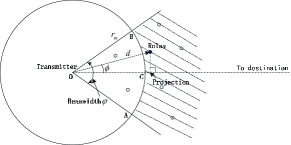
Figure 1: Selection region with the directional antenna

In a practical case, nodes are usually randomly distributed, thus relays may not be located just over the optimum transmission distance. To guarantee a relay existing at a proper position, we use the selection region based multihop routing protocol with directional antennas. For each transmitter along the route to the final destination, the selection region includes two parameters: the beamwidth $\varphi$ and a reference distance $r_{m}$, as shown in Fig. 1, where the selection region is defined as the region that is located within angle $\varphi$ and outside of the distance $r_{m}$. Here, the transmitter is located in the circle center $O$, $\angle{BOC}=\angle{AOC}=\varphi/2$, and $\overrightarrow{OC}$ points to the direction of the final destination. At each hop, the transmitter selects the nearest receiver located in the selection region as the relay.

Compared with the routing strategy using omnidirectional antennas in [1], the selection region based routing with directional antennas can be implemented much easier. Since the transmitters are equipped with directional antennas, only the receivers within the angle $\varphi$ can receive the radiated signals from the transmitters, thus the process to delimit the potential receivers within the angle $\varphi$ do not need any calculation. However, for the routing protocol with omnidirectional antennas, to determine if a receiver is located within the angle $\varphi$ or not needs a complicated calculation, e.g., calculating the angle $\phi$ between the line from the transmitter towards the final destination and the edge from the transmitter and the potential receivers, and making comparisons between these $\phi$ with $\varphi$ to decide which nodes are located within the selection region.

III Reference Distance and Transmission Probability Optimization

In this section, we derive the optimum values of the transmission probability $p$ and the reference distance $r_{m}$ for different beamwidth $\varphi$ by maximizing the expected density of progress.

III-A Upper Bound for Optimum Reference Distance

As in [4], the density of progress is defined as

$$D=p\lambda\cdot P_{s}\cdot d\cos\phi,$$

where $P_{s}$ is the successful transmission probability defined in (2), $d\cos\phi$ is the projection of the transmission distance $d$ along the line connecting the transmitter and the final destination. Since the receivers follow a homogeneous PPP with density $\lambda(1-p)$, the cumulative distribution function of the transmission distance $d$ is given as

$$\Pr(d\leq r)=1-\exp\left[-\lambda(1-p)\frac{\varphi}{2}({r^{2}}-r_{m}^{2})\right],{r_{m}}\leq r<\infty.$$ (3)

Since $\phi$ is uniformly distributed over $[-\varphi/2,\varphi/2]$, which is independent of $d$, the expected density of progress is given by

$$E[D] =p\lambda^{2}\int\limits_{r_{m}}^{\infty}\int\limits_{-\frac{\varphi}{2}}^{\frac{\varphi}{2}}{{e^{-p\frac{\varphi}{2\pi}\lambda t{x^{2}}}}}x\cos\phi{f_{d}}(x)d\phi dx$$

$$=\lambda^{2}p(1-p)\Gamma\left(\frac{3}{2},kr_{m}^{2}\right){k^{-3/2}}\exp\left(\lambda(1-p)\frac{\varphi}{2}r_{m}^{2}\right)\sin\left(\frac{\varphi}{2}\right),$$ (4)

where ${f_{d}}(x)$ is the probability density function of $d$ obtained from (4), $k=\frac{\lambda\varphi}{2}(\frac{pt}{\pi}+(1-p))$, $t$ is defined in (3a), and $\Gamma\left(\frac{3}{2},kr_{m}^{2}\right)=\int\limits_{kr_{m}^{2}}^{\infty}{{e^{-t}}{x^{\frac{3}{2}-1}}dx}$ is the incomplete Gamma function.

To optimize the objective function in (5) with respect to the beamwidth $\varphi$, let us first assume that $p$ is a constant, and try to derive the optimum value of $r_{m}$. For brevity, in the following discussion, we write the objective function as $E$. Setting the derivative with respect to $r_{m}$ as 0, after some calculations we have

$$\frac{{dE}}{{dr_{m}}}= \exp\left(\lambda(1-p)\frac{\varphi}{2}r_{m}^{2}\right)$$

$$\cdot\left[\Gamma\left(\frac{3}{2},kr_{m}^{2}\right)\lambda(1-p)\varphi r_{m}+\frac{{d\Gamma\left(\frac{3}{2},kr_{m}^{2}\right)}}{{dr_{m}}}\right]=0,$$ (5)

where $\Gamma\left(\frac{3}{2},kr_{m}^{2}\right)$ is calculated as

$$\Gamma\left(\frac{3}{2},kr_{m}^{2}\right)=\Gamma\left(\frac{3}{2}\right)+\sqrt{k}{r_{m}}\exp\left(-kr_{m}^{2}\right)-\frac{{\sqrt{\pi}}}{2}erf\left(\sqrt{k}{r_{m}}\right).$$ (6)

Therefore,

$$\frac{{d\Gamma\left(\frac{3}{2},kr_{m}^{2}\right)}}{{dr_{m}}} =\sqrt{k}\exp\left(-kr_{m}^{2}\right)\left(1-2kr_{m}^{2}\right)-\sqrt{k}\exp\left(-kr_{m}^{2}\right)$$

$$=-2{k^{3/2}}r_{m}^{2}\exp\left(-kr_{m}^{2}\right).$$ (7)

Applying (8) to (6), we obtain

$$\Gamma\left(\frac{3}{2},kr_{m}^{2}\right)\lambda\left(1-p\right)\varphi{r_{m}}-2{k^{3/2}}r_{m}^{2}\exp\left(-kr_{m}^{2}\right)=0.$$ (8)

Since it is difficult to analytically derive the exact solution for $r_{m}$ from (9), here we present an upper bound for $r_{m}$. Since

$$\Gamma\left(\frac{3}{2},kr_{m}^{2}\right) >\frac{1}{2}\left[\Gamma\left(1,kr_{m}^{2}\right)+\Gamma\left(2,kr_{m}^{2}\right)\right]$$

$$=\frac{1}{2}\exp\left(-kr_{m}^{2}\right)\left(2+kr_{m}^{2}\right),$$ (9)

using (10) in (9), we have

$$\lambda(1-p)k\varphi r_{m}^{2}-4{k^{3/2}}r_{m}+\lambda(1-p)\varphi>0.$$ (10)

Therefore,

$${r_{m}}<\frac{{2{k^{3/2}}-\sqrt{4{k^{3}}-2k{{[\lambda(1-p)\varphi]}^{2}}}}}{{k\lambda(1-p)\varphi}}.$$ (11)

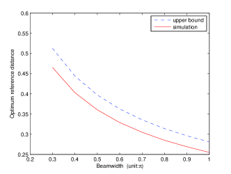
Figure 2: Numerical results and the analytical upper bound for the optimum reference distance

In Fig. 2, we compare the upper bound of the optimum $r_{m}$ with the numerical results for different beamwidth $\varphi$, when $p=0.1$.

III-B Jointly Optimizing the Reference Distance and the Transmission Probability

Now, let us maximize the objective function by jointly optimizing $r_{m}$ and $p$, for different beamwidth $\varphi$.

Rewrite (5) as

$$E=\lambda^{2}p(1-p)\exp\left(-\frac{\varphi}{2\pi}\lambda ptr_{m}^{2}\right)\Gamma\left(\frac{3}{2},kr_{m}^{2}\right)\exp\left(kr_{m}^{2}\right){k^{-3/2}}\sin\left(\frac{\varphi}{2}\right).$$

For brevity, we denote $\exp(kr_{m}^{2})$ as e and $\Gamma\left(\frac{3}{2},kr_{m}^{2}\right)$ as $\Gamma$. With partial derivatives, we have

$$\frac{{\partial E}}{{\partial r_{m}}}= \lambda^{2}p(1-p)\sin\left(\frac{\varphi}{2}\right){k^{-3/2}}\exp\left(-\frac{\varphi}{2\pi}\lambda ptr_{m}^{2}\right)$$

$$\cdot\left[-\frac{\varphi}{\pi}\lambda pt{r_{m}}\Gamma e+\Gamma\frac{{\partial e}}{{\partial r_{m}}}+e\frac{{\partial\Gamma}}{{\partial r_{m}}}\right]=0,$$ (12)

This holds only if

$$\Gamma\frac{{\partial e}}{{\partial r_{m}}}+e\frac{{\partial\Gamma}}{{\partial r_{m}}}=\frac{\varphi}{\pi}\lambda pt{r_{m}}\Gamma e.$$ (13)

Since $k=\frac{\varphi\lambda(t-\pi)}{2\pi}p+\frac{\varphi\lambda}{2}$, there is $\frac{{\partial k}}{{\partial p}}=\frac{\varphi\lambda(t-\pi)}{2\pi}$. To simplify things, we can then calculate the derivative with respect to $k$ instead of $p$ as

$$\frac{{\partial E}}{{\partial k}}=\lambda^{2}\sin\left(\frac{\varphi}{2}\right)$$

$$\cdot\left\{\left[-\frac{{tr_{m}^{2}}}{{t-\pi}}-\frac{3}{2}{k^{-1}}+\frac{{1-2p}}{{p(1-p)}}\frac{{2\pi}}{{\varphi\lambda(t-\pi)}}\right]\Gamma e+\left(\Gamma\frac{{\partial e}}{{\partial k}}+e\frac{{\partial\Gamma}}{{\partial k}}\right)\right\}=0.$$ (14)

By using the relationship $\frac{1}{2}r_{m}\frac{{\partial e}}{{\partial r_{m}}}=k\frac{{\partial e}}{{\partial k}}$, $\frac{1}{2}r_{m}\frac{{\partial\Gamma}}{{\partial r_{m}}}=k\frac{{\partial\Gamma}}{{\partial k}}$, and (14), we have

$$\Gamma\frac{{\partial e}}{{\partial k}}+e\frac{{\partial\Gamma}}{{\partial k}}=\frac{{{r_{m}}}}{{2k}}\left(\Gamma\frac{{\partial e}}{{\partial{r_{m}}}}+e\frac{{\partial\Gamma}}{{\partial{r_{m}}}}\right)=\frac{\varphi}{2\pi k}\lambda ptr_{m}^{2}\Gamma e.$$ (15)

Applying (16) to (15), the following holds:

$$\left[-\frac{{tr_{m}^{2}}}{{t-\pi}}-\frac{3}{2}{k^{-1}}+\frac{{1-2p}}{{p(1-p)}}\frac{{2\pi}}{{\varphi\lambda(t-\pi)}}\right]\Gamma e+\frac{\varphi}{{2k\pi}}\lambda ptr_{m}^{2}\Gamma e=0.$$ (16)

After some calculation, we have

$$-\frac{{\varphi t}}{{2(t-\pi)}}\lambda r_{m}^{2}-\frac{3}{2}+\frac{{[p+\pi/(t-\pi)](1-2p)}}{{p(1-p)}}=0.$$ (17)

Given beamwidth $\varphi$, we use $\varphi$ and the optimum $p$ to express the optimum $r_{m}$ as

$${r_{m}}=\frac{1}{{\sqrt{\varphi\lambda}}}\sqrt{\frac{{2[p(t-\pi)+\pi](1-2p)}}{{p(1-p)t}}-\frac{{3(t-\pi)}}{t}}.$$ (18)

Interestingly, by jointly optimizing $r_{m}$ and $p$, we find that the optimum transmission probability $p$ in (19) is a constant independent of beamwidth $\varphi$, which is different from the result we had in [1]. The proof is shown in Appendix.

Since in (19) $p$ is an constant, $r_{m}$ is only related to the beamwidth $\varphi$. Thus for a given beamwidth $\varphi$, there is an associated optimum reference distance $r_{m}$ for the transmitters to select next hop relay node, as shown in Fig. 4. Also note that in (19) $r_{m}$ scales as $\lambda^{-1/2}$, which intuitively makes sense. This is because as the node density increases, the interferers’ relative distance to the receiver decreases as $\sqrt{\lambda}$, it requires a shorter transmission distance by the same amount to keep the required SINR. By applying (19) in (5), we observe that (5) becomes $N\sqrt{\lambda}$, where $N$ is a constant independent of $\lambda$. This means that the maximum expected density of progress scales as $\Theta(\sqrt{\lambda})$, which conforms to the results in [2] and [6].

IV Numerical Results and Interpretations

In this section, we present some numerical results based on the analysis in Section III. We choose the path-loss exponent $\alpha$ as 3, the node density $\lambda$ as 1, and the outage threshold $\beta$ as 10 dB.

In Fig. 3, we show the optimum transmission probability obtained numerically vs. the beamwidth $\varphi$. As shown in the figure, the optimum transmission probability $p$ is a constant, which does not change with the beamwidth $\varphi$, this confirms our proof in Appendix. Thus, with the selection region based routing with directional antennas, no matter how much the directional antenna’s beamwidth we select, the optimum transmission probability always keeps the same as $p=0.12$. However, when we use the routing strategy with omnidirectional antenna, the optimum transmission probability $p$ changes with the selection angle $\varphi$ (see Fig. 5 in [1]).

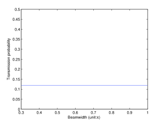
Figure 3: The optimum transmission probability $p$ vs. the beamwidth $\varphi$

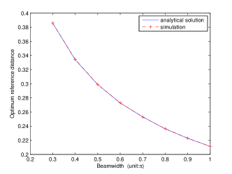
Figure 4: The optimum reference distance vs. the beamwidth $\varphi$

In Fig. 4, we compare the optimum reference distance $r_{m}$ obtained numerically with that derived in (19), where $p$ is chosen optimally as the constant shown in Fig. 3. We see that increment of the beamwidth $\varphi$ leads to the decease of the optimum reference distance. This can be explained as follows: Increment of the beamwidth $\varphi$ means more interference seen by a receiver; therefore, the optimum reference transmission distance should be decreased to guarantee the quality of the received signal and the transmission successful probability.

In Fig. 5, we compare the expected density of progress of the routing protocol using directional antennas with that using omnidirectional antennas in [1]. From the figure, we see that the expected density of progress for selection region based routing with directional antennas owns a great advantage to that of the routing strategy with omnidirectional antennas. This is because directional antennas can bring benefits such as reduced interference and increased spatial reuse compared with omnidirectional antennas.

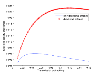
Figure 5: Comparison of the expected density of progress for the routing protocol using directional antennas with that using omnidirectional antennas

V Conclusions

We propose a selection region based multihop routing protocol for wireless ad hoc networks with directional antennas, where the selection region is defined by the beamwidth and the reference distance. By maximizing the expected density of progress, we present some analytical results on how to refine the selection region and the transmission probability. Compared with the routing strategy with omnidirectional antennas in [1], the routing protocol in this paper owns two main advantages: higher expected density of progress and less computational complexity when choosing the next hop relay.

Here, we prove that when jointly optimizing the reference distance $r_{m}$ and the transmission probability $p$, the optimum transmission probability $p$ is a constant independent of beamwidth $\varphi$.

Step 1: We consider the partial derivitive to the reference distance $r_{m}$, which is shown in (9), here rewrite as

$$\Gamma\left(\frac{3}{2},kr_{m}^{2}\right)\lambda\left(1-p\right)\varphi{r_{m}}-2{k^{3/2}}r_{m}^{2}\exp\left(-kr_{m}^{2}\right)=0,$$ (19)

where $k=\frac{\lambda\varphi}{2}\left(\frac{pt}{\pi}+(1-p)\right)$. Applying $k$ to (20), we have

$$\Gamma\left(\frac{3}{2},kr_{m}^{2}\right)\left(1-p\right)-\left[\frac{pt}{\pi}+(1-p)\right]\sqrt{{k}r_{m}^{2}}\exp\left(-kr_{m}^{2}\right)=0.$$ (20)

Step 2: Now let us focus on the partial derivitive to the transmission probability $p$. As mentioned in Section III-B, we calculate the derivitive with respect to $k$ instead, here rewrite (15) as

$$\frac{{\partial E}}{{\partial k}}=\lambda^{2}\sin(\frac{\varphi}{2})$$

$$\cdot\left\{\left[-\frac{{tr_{m}^{2}}}{{t-\pi}}-\frac{3}{2}{k^{-1}}+\frac{{1-2p}}{{p(1-p)}}\frac{{2\pi}}{{\varphi\lambda(t-\pi)}}\right]\Gamma e+\left(\Gamma\frac{{\partial e}}{{\partial k}}+e\frac{{\partial\Gamma}}{{\partial k}}\right)\right\}=0.$$ (21)

By using the same notation, defined in Section III-B, i.e., $e=\exp\left(kr_{m}^{2}\right)$ and $\Gamma=\Gamma\left(\frac{3}{2},kr_{m}^{2}\right)$, we have

$$\frac{{\partial e}}{{\partial k}}=\exp(kr_{m}^{2})r_{m}^{2}.$$ (22)

$$\frac{{\partial\Gamma}}{{\partial k}}=-k^{\frac{1}{2}}r_{m}^{3}\exp(kr_{m}^{2}).$$ (23)

Applying (23) and (24) to (22), we have

$$\left[-\frac{{tkr_{m}^{2}}}{{t-\pi}}-\frac{3}{2}+\frac{{1-2p}}{{p(1-p)}}\frac{pt+\pi(1-p)}{{(t-\pi)}}\right]\Gamma e$$

$$+\Gamma\exp\left(kr_{m}^{2}\right)kr_{m}^{2}-\left(kr_{m}^{2}\right)^{\frac{3}{2}}=0.$$ (24)

Step 3: Applying (19) to (21) and (25), we see that in $kr_{m}^{2}$, $\varphi$ can be cancelled, thus (21) and (25) become two equations that are independent of $\varphi$. Therefore, when jointly optimizing $r_{m}$ and $p$, the optimum $p$ is a constant independent of the beamwidth $\varphi$, only related to $t$ which is defined in (3a). And the numerical value for the optimum $p$ is given in Fig. 3.

References

- [1] D. Li, C. Yin, C. Chen, and S. Cui,“A Selection Region Based Routing Protocol for Random Mobile ad hoc Networks,”IEEE Globecom2010 Workshop on Heterogeneous, Multi-Hop, Wireless and Mobile Networks, Dec. 2010, accepted. [Online] Available: http://arxiv.org/abs/1007.3105.
- [2] P. Gupta and P. R. Kumar, “The capacity of wireless networks,” IEEE Transactions on Information Theory, vol. 46, no. 2, pp. 388–404, Mar. 2000.
- [3] S. Weber, X. Yang, J. G. Andrews, and G. de Veciana, “Transmission capacity of wireless ad hoc networks with outage constraints,” IEEE Transactions on Information Theory, vol. 51, no. 12, pp. 4091–4102, Dec. 2005.
- [4] F. Baccelli, B. Blaszczyszyn, and P. Muhlethaler, “An Aloha protocol for multihop mobile wireless networks,” IEEE Transactions on Information Theory, vol. 52, no. 2, pp. 421–436, Feb. 2006.
- [5] S. Weber, N. Jindal, R.K. Ganti, and M. Haenggi, “Longest Edge Routing on the Spatial Aloha Graph,” Proceedings of the IEEE GLOBECOM, pp. 1-5, Nov. 2008.
- [6] J. G. Andrews, S. Weber, M. Kountouris and M. Haenggi, “Random Access Transport Capacity,” IEEE Transactions On Wireless Communications, submitted. [Online] Available: http://arxiv.org/ps_cache/arxiv/pdf/0909/0909.5119v1.pdf.
- [7] S. Yi and Y. Pei and S. Kalyanaraman, “On the capacity improvement of ad hoc wireless networks using directional antennas,” Proceedings of Mobihoc ,2003.
- [8] A. Spyropoulos, and C.S. Raghavendra,“Capacity bounds for ad-hoc networks using directional antennas,”Proceedings of IEEE ICC , vol. 1, pp.348 - 352, May. 2003.
- [9] H. Dai, K. Ng, R. Wong, and M. Wu,“On the Capacity of Multi-Channel Wireless Networks Using Directional Antennas,”Proceedings of the IEEE INFOCOM, pp.628 -636, Apr. 2008.