Radiative transfer in ultra-relativistic outflows

Abstract

Analytical and numerical solutions are obtained for the equation of radiative transfer in ultra-relativistic opaque jets. The solution describes the initial trapping of radiation, its adiabatic cooling, and the transition to transparency. Two opposite regimes are examined: (1) Matter-dominated outflow. Surprisingly, radiation develops enormous anisotropy in the fluid frame before decoupling from the fluid. The radiation is strongly polarized. (2) Radiation-dominated outflow. The transfer occurs as if radiation propagated in vacuum, preserving the angular distribution and the blackbody shape of the spectrum. The escaping radiation has a blackbody spectrum if (and only if) the outflow energy is dominated by radiation up to the photospheric radius.

1. Introduction

Powerful jets from compact objects can have significant optical depth to scattering. The foremost example is gamma-ray bursts (GRBs). They are emitted by hot ultra-relativistic outflows that remain opaque until they travel a large distance from the central engine. Where the jet becomes transparent, the trapped radiation is released and contributes to the GRB. Its spectrum is expected to be nonthermal because of dissipative processes in the subphotospheric region.

This “photospheric emission” is likely the main component of observed GRBs. Recent work provides significant support for this picture. Three heating mechanisms have been proposed to shape the photospheric spectrum: (1) internal shocks, (2) dissipation of magnetic energy and excited plasma waves (Thompson 1994; Spruit, Daigne, & Drenkhahn 2001; Ioka et al. 2007), and (3) collisional dissipation (Beloborodov 2010; hereafter B10). The latter mechanism is straightforward to model from first principles and turns out to reproduce the canonical GRB spectrum with no fine-tuning of parameters (B10; Vurm, Beloborodov, & Poutanen 2011).

Modeling emission from opaque jets requires simulations of radiative transfer. Two methods have been developed for such simulations to date. First, solving the kinetic equations for the electrons and photons that interact via Compton scattering (Pe’er & Waxman 2005; Vurm et al. 2011). Second, tracking a large number of photons that propagate and (randomly) scatter in the jet (Giannios 2006; B10). Pe’er (2008) used an analytic approach and Monte-Carlo simulations to study individual short pulses of photospheric emission.

None of these works attempted to use the standard transfer equation. This approach is developed in the present paper. The extension of radiative transfer theory to relativistic outflows is straightforward (e.g. Castor 1972; Mihalas 1980). In Section 2, we write down the transfer equation that is well-behaved (and simplifies) in the ultra-relativistic regime. Then we solve this equation for isotropic (Section 3) and exact (Section 4) models of electron scattering. In parallel, we apply the independent Monte-Carlo technique and compare the results.

In Section 5 we separately consider the case where radiation dominates the outflow energy up to the photosphere. This regime is of interest for GRBs with extremely low baryon loading, as described by Paczyński (1986) and Goodman (1986). In contrast to their expectations, the transfer near the photosphere is not complicated and has a simple analytical solution.

2. Transfer equation in the ultra-relativistic regime

2.1. Formulation of the problem

We are interested in outflows with Lorentz factors $\Gamma\gg 1$ and velocities $\beta=v/c\rightarrow 1$. Below we consider radiative transfer in outflows that are steady and spherically symmetric. These assumptions are not restrictive in the ultra-relativistic regime, as discussed in Section 6, — even strongly variable and beamed jets may be described by this model.

The transfer equation is well-behaved in the limit $\beta\rightarrow 1$ when it is formulated for radiation intensity in the fluid frame (see Appendix A). This frame is comoving with the outflow at any radius $r$. Hereafter intensity is denoted by $I_{\nu}(r,\mu,\nu)$ where $\nu$ is the photon frequency, $\mu=\cos\theta$, and $\theta$ is the photon angle with respect to the radial direction. The quantities $\nu$, $\mu$, and $I_{\nu}$ are measured in the fluid frame. When $\beta\rightarrow 1$, the transfer equation (A11) simplifies to

$$\frac{\partial I_{\nu}}{\partial\ln r} = -\left(1-\mu^{2}\right)g\,\frac{\partial I_{\nu}}{\partial\mu}+(1-\mu g)\left(\frac{\partial I_{\nu}}{\partial\ln\nu}-3I_{\nu}\right)$$ (1)

$$+ \tau_{\nu}\,\frac{(S_{\nu}-I_{\nu})}{1+\mu},$$

where

$$g(r)\equiv 1-\frac{d\ln\Gamma}{d\ln r}.$$ (2)

The quantity $S_{\nu}$ appearing in equation (1) is the source function in the fluid frame. It is determined by how radiation interacts with the outflow. For example, the simplest model of isotropic and coherent scattering gives $S_{\nu}=(1/2)\int I_{\nu}\,d\mu$ (e.g. Chandrasekhar 1960).

The quantity $\tau_{\nu}$ in equation (1) approximately represents the outflow optical depth (cf. Appendix B). It is defined as $\tau_{\nu}\equiv\kappa_{\nu}r/\Gamma$ where $\kappa_{\nu}$ is the opacity in the fluid frame. In GRB jets, electron/positron scattering strongly dominates the opacity around the spectral peak of the burst. The scattering opacity is $\kappa_{\nu}=\sigma n$ where $\sigma$ is the scattering cross section and $n$ is the proper $e^{\pm}$ density of the flow. It may be expressed in terms of the rate of $e^{\pm}$ outflow through the sphere $4\pi r^{2}$ in the lab frame, $\dot{N}_{e}=4\pi r^{2}\,n\,\Gamma\,\beta c$. Then $\tau_{\nu}$ is given by

$$\tau_{\nu}=\frac{\sigma\,\dot{N}_{e}}{4\pi r\,\Gamma^{2}\,\beta c}.$$ (3)

When the outflow carries no positrons, $\dot{N}_{e}$ remains constant with radius. It also remains constant if positron creation is balanced by annihilation (this situation takes place in collisionally heated jets, see B10).

Besides the simpler form of the transfer equation, the ultra-relativistic regime implies a principal change in the formulation of the transfer problem. Radiation in the lab frame is strongly collimated and essentially all photons stream outward. Inward radial motion in the lab frame requires $\mu<-\beta$ in the fluid frame, which corresponds to a small solid angle $\Delta\Omega=2\pi(1-\beta)$. At any given radius, only a small fraction ${\cal O}(\Gamma^{-2})$ of all photons have $\mu<-\beta$. As long as $\Gamma\gg 1$, one can exclude the solid angle $\mu<-\beta$ from the transfer problem, i.e. neglect its contribution ${\cal O}(\Gamma^{-2})$ when calculating the source function $S_{\nu}$, and solve the problem in the domain $-\beta<\mu<1$. Then the outer boundary condition is not needed, as information cannot propagate from larger $r$ to small $r$.

Thus, only an inner boundary condition should be specified for the ultra-relativistic transfer problem. If it is given at a sufficiently small radius $r_{\rm in}$, the radiation may be assumed isotropic in the fluid frame (as demonstrated by the solutions presented below, radiation maintains isotropy where $\tau_{\nu}>100$).

Equation (1) uses radius $r$ as an independent variable. Alternatively, it can be written in terms of the comoving-observer time $t(r)$ which is related to $r$ by $dt=dr/\beta c\Gamma$. Then the transfer problem takes the form of an initial-value problem. One can think of ultra-relativistic transfer as the evolution of intensity $I(\mu)$, as seen by the comoving observer. This view is valid as long as radiation is not allowed to stream backward in time $t$ (i.e. backward in $r$). The model is exact in the limit $\Gamma\rightarrow\infty$ (then the entire region $-1<\mu<1$ is included in the transfer domain without violating causality). In practice, equation (1) and the neglect of photons with $\mu<-\beta$ gives an excellent approximation when $\Gamma>10$. The approximation is perfect for GRB jets.

2.2. Transfer of energy

The flow of radiation energy is described by the frequency-integrated intensity,

$$I(\mu,r)=\int_{0}^{\infty}I_{\nu}\,d\nu,\qquad S(\mu,r)=\int_{0}^{\infty}S_{\nu}\,d\nu.$$ (4)

Integration of equation (1) over $\nu$ gives the equation for $I(\mu,r)$,

$$\frac{\partial I}{\partial\ln r}=-\left(1-\mu^{2}\right)\,g\,\frac{\partial I}{\partial\mu}-4\,(1-\mu g)\,I+\tau\,\frac{(S-I)}{1+\mu},$$ (5)

where $\tau(r)=\Gamma^{-1}\kappa(r)r$ is defined using the effective opacity, $\kappa=I^{-1}\int\kappa_{\nu}\,I_{\nu}\,d\nu$.

Multiplying equation (5) by $1+\mu$ and integrating over $\mu$, one gets

$$\frac{d(I_{0}+I_{1})}{d\ln r}=-4(I_{0}+I_{1})+g\left(I_{0}+2I_{1}+I_{2}\right)+\tau\,(S_{0}-I_{0}),$$ (6)

where $I_{m}$ ($m=0,1,2$) are the moments of intensity,

$$I_{m}(r)=\frac{1}{2}\int_{-1}^{1}I(\mu,r)\,\mu^{m}\,d\mu,$$ (7)

and $S_{0}(r)$ is the zero moment of the source function. The quantities $4\pi I_{m}$ are the components of the stress-energy tensor of radiation, and equation (6) in essence expresses the first law of thermodynamics for radiation (e.g. Castor 1972).

In the case of coherent scattering (e.g. Thomson scattering by a plasma with a small Kompaneets’ $y$-parameter) $S_{0}=I_{0}$. Then the last term in equation (6) vanishes — there is no heat exchange between the plasma and radiation, and the evolution of radiation with $r$ is adiabatic. Radiation does $PdV$ work and gradually gives away energy to the bulk kinetic energy of the outflow as it propagates to larger radii. This process of adiabatic cooling is easily described at large optical depths, $\tau\gg 1$, where radiation is nearly isotropic in the fluid frame, $I_{1}=0$ and $I_{2}=I_{0}/3$. Then equation (6) gives

$$\frac{d\ln I_{0}}{d\ln r}=-4+\frac{4}{3}\,g.$$ (8)

This equation reproduces the law of adiabatic cooling of radiation (adiabatic index $4/3$) in expanding volume. For example, if $\Gamma(r)=const$ ($g=1$, see eq. 2) volume expands as $r^{-2}$ and radiation energy density in the fluid frame $U=4\pi I_{0}/c$ decreases as $r^{-8/3}$. The energy flux through the sphere $4\pi r^{2}$ measured in the lab frame decreases as $r^{-2/3}$. Note that equation (8) is valid only if radiation is isotropic in the fluid frame. Strong deviations from isotropy (which occur at optical depths $\tau\mathrel{\hbox{\raise 2.15277pt\hbox{$<$}\hbox to0.0pt{\hss\lower 2.15277pt\hbox{$\sim$}}}}10$ as shown below) change the rate of adiabatic cooling.

The fact that radiation does work on the outflow implies that the outflow accelerates and $g$ in equation (1) is not an independent parameter of the transfer problem. It may be treated as a given fixed parameter only if the outflow inertia is large enough, so that it cannot be significantly accelerated by radiation. This condition reads $\rho c^{2}\gg U$ where $\rho$ is the rest-mass density of the outflow. This condition will be assumed in Sections 3 and 4, where we solve the transfer equation with $g\approx 1$ [i.e. $\Gamma(r)\approx const$]. In Section 5, we consider the opposite regime and discuss the coupled dynamics of the outflow and radiation.

2.3. Transfer of photon number

The photon number intensity is described by the following quantity,

$${\cal I}(\mu,r)=\int_{0}^{\infty}\frac{I_{\nu}}{h\nu}\,d\nu,$$ (9)

where $h$ is Planck constant. Integration of equation (1) over $d\ln\nu$ gives the equation for ${\cal I}(\mu,r)$,

$$\frac{\partial{\cal I}}{\partial\ln r}=-\left(1-\mu^{2}\right)\,g\,\frac{\partial{\cal I}}{\partial\mu}-3\,(1-\mu g)\,I+\tau\,\frac{({\cal S}-{\cal I})}{1+\mu},$$ (10)

where ${\cal S}=\int(S_{\nu}/h\nu)\,d\nu$ and $\tau(r)=\Gamma^{-1}\kappa(r)r$ is defined using $\kappa={\cal I}^{-1}\int\kappa_{\nu}\,{\cal I}\,d\nu$.

Scattering conserves photon number, and the transfer equation is expected to give the corresponding conservation law. Multiplying equation (10) by $1+\mu$, integrating over $\mu$, and re-arranging terms, one gets

$$\frac{d}{d\ln r}\,\ln\left[\Gamma({\cal I}_{1}+{\cal I}_{0})\right]=-2,$$ (11)

where ${\cal I}_{m}(r)$ are the moments of ${\cal I}(\mu,r)$ and we used ${\cal I}_{0}={\cal S}_{0}$ which is true for any scattering process. The quantity $4\pi{\cal I}_{1}$ is the number flux of photons measured in the fluid frame, and $4\pi{\cal I}_{0}/c$ is the number density of photons in the fluid frame. Lorentz transformation of the four-flux vector $4\pi({\cal I}_{0},{\cal I}_{1},0,0)$ gives the radial photon flux measured in the lab frame, $\tilde{\cal F}=4\pi\Gamma({\cal I}_{1}+\beta{\cal I}_{0})$. Equation (11) in essence states $r^{2}\tilde{\cal F}=const$ (with $\beta\rightarrow 1$) and expresses conservation of photon number.

3. Isotropic-scattering model

In this section, we solve the transfer problem assuming the simplest form of the interaction between radiation and the fluid: coherent isotropic scattering in the fluid frame. It gives a reasonable first approximation to Thomson scattering that is considered in Section 4. We consider here matter-dominated outflows — the outflow is assumed to be massive enough, so that it can coast with $\Gamma(r)\approx const$ (Section 2.2), which corresponds to $g(r)\approx 1$ (eq. 2).

Then the energy transfer equation (5) reads,

$$\frac{\partial I}{\partial\ln r}=-\left(1-\mu^{2}\right)\,\frac{\partial I}{\partial\mu}-4(1-\mu)\,I+\tau\,\frac{(I_{0}-I)}{1+\mu}.$$ (12)

Here we substituted the source function that describes isotropic scattering $S(\mu,r)=I_{0}(r)$, where $I_{0}$ is the zero-moment of intensity (eq. 7). We will assume a constant cross section $\sigma(\nu)=const$ and $\dot{N}_{e}(r)=const$. Then equation (3) gives

$$\tau(r)=\frac{R_{\star}}{r},\qquad R_{\star}=\frac{\sigma\,\dot{N}_{e}}{4\pi\,\Gamma^{2}\,\beta c}.$$ (13)

Transfer of photon number is described by equation similar to equation (12) where $I$ is replaced by ${\cal I}$ and the numerical coefficient $-4$ in the second term on the right-hand side is replaced by $-3$ (cf. eq. 10).

3.1. Integration of transfer equation

Equation (12) gives the expression for $\partial I/\partial\ln r$ in terms of $I$. Direct integration in $\ln r$ immediately yields the solution for $I(\mu,r)$. Our numerical integration starts at $r_{\rm in}=3\times 10^{-3}R_{\star}$ and takes the isotropic $I(\mu,r_{\rm in})=const$ as the boundary condition. We use a uniform grid in $\theta$ and $\ln r$ of size $300\times 10^{5}$. With a simplest integrator — Runge-Kutta scheme of fourth order — the grid gives excellent accuracy of $\sim 0.1$% (we have checked this by varying the grid). Two more details of numerical integration are worth mentioning:

(1) At one boundary of the computational domain $\mu\rightarrow-1$ and the transfer equation gives $(S-I)/I\rightarrow 0$. This requires $I=S=I_{0}$ at $\mu=-1$. Note that the optical depth $\Delta\tau_{\rm ray}$ passed along the ray in one step $\Delta\ln r$ depends on $\mu$: $\Delta\tau_{\rm ray}(\mu)=\tau(r)\,\Delta\ln r/(1+\mu)$. Numerical integration is possible only if $\Delta\tau_{\rm ray}<1$, which is violated close to the boundary $\mu=-1$. However, in this region $\tau_{\rm ray}=\tau/(1+\mu)\gg 1$ simply enforces $I\approx S$. In the process of integration, we set $I=S$ wherever $\Delta\tau_{\rm ray}(\mu)>0.7$.

(2) The transfer equation contains the term $(1-\mu^{2})\,\partial I/\partial\mu=\sin\theta\,\partial I/\partial\theta$. We use a grid $\theta_{i}$ ($i=0,...,n$), where $\theta_{0}=0$ and $\theta_{n}=\pi$. The term $\sin\theta\,\partial I/\partial\theta$ is not needed at $\theta_{0}$ and $\theta_{n}$ (it vanishes). For all other $\theta_{i}$ we evaluate this term using $\partial I/\partial\theta=(I_{i+1}-I_{i-1})/(\theta_{i+1}-\theta_{i-1})$.

The transfer equation (12) has no free parameters and the solution is unique. The result is shown in Figure 1. The striking feature is the strong beaming of the radiation field in the fluid frame, even at large optical depths $\tau\sim 10$. Beaming may be described by the ratio of intensities at $\mu=1$ and $\mu=-1$: $b(r)\equiv I(1,r)/I(-1,r)$. This quantity is shown in Figure 2. It significantly deviates from unity starting at $\tau\sim 10$. In the zone of $\tau\ll 1$, $I(1,r)=const$ and $I(-1,r)=I_{0}\propto r^{-2}$. Therefore $b(r)\propto r^{2}$ at $r\gg R_{\star}$.

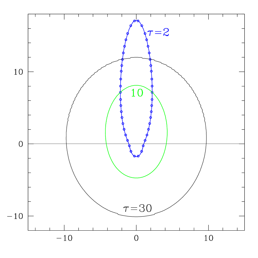
Figure 1.— Angular distribution of radiation intensity in the fluid frame at three radii: $r/R_{\star}\approx 0.03$, 0.1 and 0.5, which correspond to optical depths $\tau\approx 30$, 10, and 2, respectively. For a better comparison, we plot $(r/R_{\star})^{2}I$, where the factor $(r/R_{\star})^{2}$ compensates for the photon dilution due to expansion. The overall normalization of the transfer solution is chosen so that $I(\mu,r)=(r/R_{\star})^{-8/3}=\tau^{8/3}$ at radii $r<0.01R_{\star}$ where radiation is nearly isotropic ($I$ does not depend on $\mu$) and follows the adiabatic cooling law $I=\tau^{8/3}$. Open circles show the intensity at $\tau=2$ that is obtained by the Monte-Carlo code (Section 3.3).

Figure 2.— Beaming factor $b(r)=I(1,r)/I(-1,r)$ in the fluid frame. Dashed curve shows the model with isotropic coherent scattering. Solid curve shows the model with Thomson scattering in a cold outflow (Section 4.1).

3.2. Adiabatic cooling

To examine adiabatic cooling, one should consider the energy flux of radiation in the lab frame $\tilde{F}=4\pi\tilde{I}_{1}$, where $\tilde{I}_{1}=\Gamma^{2}[\beta(I_{0}+I_{2})+(1+\beta^{2})I_{1}]$ is the first moment of intensity in the lab frame. Here we cannot take the formal limit $\Gamma\rightarrow\infty$, as the transformation between the lab frame and the fluid frame is not well defined in this limit. The total luminosity of radiation measured in the lab frame is

$$L(r)=4\pi r^{2}\tilde{F}=(4\pi)^{2}\,r^{2}\,\Gamma^{2}\,\left[\beta\left(I_{0}+I_{2}\right)+\left(1+\beta^{2}\right)I_{1}\right].$$ (14)

Freely streaming radiation would have $L(r)=const$. Interaction with the outflow results in adiabatic cooling and $L(r)$ decreases with $r$.

The adiabatic cooling factor is defined by $a(r_{\rm in}\rightarrow r)=L(r)/L(r_{\rm in})$. We chose $r_{\rm in}\ll R_{\star}$ where radiation is nearly isotropic; then $I_{1}(r_{\rm in})=0$ and $I_{2}(r_{\rm in})=I_{0}(r_{\rm in})/3$. This gives,

$$a(r_{\rm in}\rightarrow r)\equiv\frac{L(r)}{L(r_{\rm in})}=\frac{3}{4}\,\frac{r^{2}}{r_{\rm in}^{2}}\,\frac{\beta\left(I_{0}+I_{2}\right)+\left(1+\beta^{2}\right)I_{1}}{I_{0}(r_{\rm in})}.$$ (15)

This equation is well-behaved in the limit $\beta\rightarrow 1$. Adiabatic cooling is controlled by $I_{0}(r)$, $I_{1}(r)$, and $I_{2}(r)$, which we know from the solution of the transfer equation. Figure 3 shows the resulting $a$. In the deep subphotospheric region (where radiation is approximately isotropic in the fluid frame) $a=(r/r_{\rm in})^{-2/3}$ as expected. A deviation from this law develops at $\tau\sim 10$ (see also Monte-Carlo simulations in Pe’er 2008). In the region $\tau\ll 1$ ($r\gg R_{\star}$) most of radiation streams freely and experiences no adiabatic cooling.

The net effect of adiabatic cooling on the escaping radiation is described by

$$a(r_{\rm in}\rightarrow\infty)=2\,\left(\frac{r_{\rm in}}{R_{\star}}\right)^{2/3}=2\,\tau_{\rm in}^{-2/3}.$$ (16)

Figure 3.— Adiabatic cooling factor $a(r_{\rm in}\rightarrow r)$. We multiplied $a$ by $(R_{\star}/r_{\rm in})^{2/3}$ in this plot; this combination does not depend on $r_{\rm in}$ as long as $r_{\rm in}\ll R_{\star}$. Dotted line shows the thermodynamic result $a=(r/R_{\star})^{-2/3}$, which is valid for approximately isotropic radiation. The actual cooling factor obtained from the transfer solution is shown by the solid and dashed curves. Dashed curve: model with isotropic coherent scattering. Solid curve: model with Thomson scattering in a cold outflow (Section 4.1).

3.3. Monte-Carlo simulation

As an independent check of the results presented above, we solved the same transfer problem using the Monte-Carlo method. The numerical code is described in B10. In this section, we use its simplest version that assumes coherent isotropic scattering in the fluid frame.

The Monte-Carlo method is fundamentally different from solving the transfer equation. It operates with individual photons that are injected at $r_{\rm in}\ll R_{\star}$. The simulation assumes a finite $\Gamma$ and is performed in the lab frame. It tracks the propagation and random scattering of a large number of injected photons and accumulates their statistics at different radii. These statistics are used to reconstruct the angular distribution of radiation intensity in the fluid frame. We ran the Monte-Carlo simulation for outflows with $\Gamma=20$ and $\Gamma=600$. The results were identical, again confirming that the transfer does not depend on $\Gamma$ as long as $\Gamma\gg 1$ and $\Gamma(r)=const$.

To reconstruct the radiation intensity at a given radius $r$ from the Monte-Carlo simulation, we calculate the angular distribution of luminosity passing through the sphere of radius $r$ in the lab frame, $dL/d\tilde{\mu}\,(r)$. In the ultra-relativistic transfer problem, practically all photons move forward in radius and cross a given $r$ only once. We accumulate the statistics of angles and energies of photons at radius $r$, which gives $dL/d\tilde{\mu}$ and the intensity of radiation in the lab frame, $\tilde{I}=(4\pi r^{2}\tilde{\mu})^{-1}dL/d\tilde{\mu}$. The corresponding intensity in the fluid frame is given by $I={\cal D}^{-4}\tilde{I}$ where ${\cal D}$ is the Doppler factor (eq. A3). Open circles in Figure 1 show the result of this calculation at $r=R_{\star}/2$. It is in perfect agreement with the solution of the transfer equation. Similar excellent agreement is found at other radii.

The strong anisotropy of radiation at subphotospheric radii is a result of cooperating effects. Photons with large $\mu$ have a larger free path in the lab frame $\lambda$ (in the opaque zone, $\lambda\approx[1+\beta\mu]\,r/\tau$.) The free path is accompanied by a shift in $\mu$, $\Delta\mu=(d\mu/ds)\,\lambda>0$. This leads to the pile up of photons along the radial direction. Photons with large $\mu$ also experience less adiabatic cooling than the more frequently scattered photons with small $\mu$.

3.4. Fuzzy photosphere

$R_{\star}$ was defined in equation (13) as the radius where the parameter $\tau$ appearing in the transfer equation equals unity. It gives an estimate for the characteristic photospheric radius. Clearly, the sphere of radius $R_{\star}$ cannot be thought of as the last-scattering surface, for two reasons: (1) the optical depth seen by a photon depends on its emission angle $\mu=\cos\theta$ and (2) the free path of a photon near $R_{\star}$ is a random variable comparable to $R_{\star}$. Therefore, the radius of last scattering $r_{\star}$ is a random variable. Its average value logarithmically diverges for a steady outflow extending to infinity and cannot be used to define the photosphere.

The process of radiation decoupling from the scattering plasma may be described by the probability distribution $dP/dr_{\star}d\mu_{\star}$ where $\mu_{\star}=\cos\theta_{\star}$ is the emission angle of the photon (measured in the fluid frame) at the last-scattering point. Pe’er (2008) considered a similar distribution for $r_{\star}$ and $\tilde{\theta}_{\star}$, where $\tilde{\theta}_{\star}$ is the emission angle in the lab frame. His analytical expression is however inaccurate. The correct expression is given in Appendix B. Integrating $dP/dr_{\star}d\mu_{\star}$ over $\mu_{\star}$, one finds the distribution of emitted photons over the radius of last scattering, $dP/dr_{\star}$ (Fig. 4).

The same $dP/dr_{\star}$ is obtained using Monte-Carlo technique. The advantage of the Monte-Carlo simulation is that it is easily extended to hot outflows and to scattering with exact Compton cross section. We calculated $dP/d\ln r_{\star}$ for the collisionally heated jet in the model of B10. The result was practically identical to that shown in Figure 4.

Figure 4.— Distribution of the last-scattering radius $r_{\star}$, obtained by integrating equation (B16) over $\mu_{\star}$. Identical distribution is obtained using the Monte-Carlo technique. The distribution remains practically the same in all models of photon transfer calculated in this paper: isotropic scattering, Thomson scattering in cold plasma, and Compton scattering in hot plasma. Approximately 2/3 of photons have $r_{\star}$ between $0.3R_{\star}$ and $3R_{\star}$.

In view of the broad distribution of $r_{\star}$, it is not appropriate to locate the GRB photosphere at any specific radius, as emphasized by Pe’er (2008). When a characteristic radius is needed for rough estimates, $R_{\star}$ would be a reasonable choice. Alternatively, a characteristic photosphere could be defined as the sphere outside of which 50% of photons are released (i.e. experience the last scattering). The corresponding radius is $0.8R_{\star}$.

4. Transfer with exact electron scattering

Even for cold outflows, the radiative transfer is not exactly described by the model of coherent isotropic scattering. Two effects contribute to this: (1) electron scattering is not isotropic, and (2) radiation becomes polarized in the process of radiative transfer, with two modes of polarization, so two equations describe the transfer problem instead of one.

Furthermore, if the outflow is strongly heated (as expected in GRBs) scattering is not coherent, i.e. does not conserve photon energy in the fluid frame. This has a strong effect on the intensity of radiation, as instead of passive adiabatic cooling radiation is heated through the Comptonization process.

In Section 4.1 we develop the accurate transfer model for Thomson scattering in a cold outflow, which takes into account polarization. In Section 4.2 we present a transfer model for heated outflows. The results are compared with the simple isotropic-scattering model of Section 3.

4.1. Thomson scattering and polarization

The polarized transfer in a static, cold electron medium was described by Chandrasekhar (1960) and Sobolev (1963). In axisymmetric problems, e.g. in plane-pallel or spherical geometries, there are two polarization modes of radiation: one with electric field perpendicular to the plane containing the photon direction and the axis of symmetry and the other with electric field parallel to this plane. Let $I_{\perp}$ and $I_{\parallel}$ be the energy intensities of the two modes. Scattering can change the polarization state, so four scattering processes can occur: $\perp\rightarrow\perp$, $\perp\rightarrow\parallel$, $\parallel\rightarrow\perp$, and $\parallel\rightarrow\parallel$. They are described by four different cross-sections. The total intensity of radiation is $I=I_{\perp}+I_{\parallel}$. The degree of polarization is $p=Q/I$ where $Q=I_{\perp}-I_{\parallel}$.

The transfer equations for $I$ and $Q$ in a static medium are given in Chandrasekhar (1960) and Sobolev (1963). The generalization of these equations to the case of a relativistically moving medium is straightforward (see Beloborodov 1998 for equations in the plane-parallel geometry). Here we are interested in spherical ultra-relativistic outflows. We will use the corresponding equations for the intensities in fluid frame, which are well-behaved in the limit $\beta\rightarrow 1$. The transfer equations for $I$ and $Q$ are similar to equation (5),

$$\frac{\partial I}{\partial\ln r}=-\left(1-\mu^{2}\right)\,g\,\frac{\partial I}{\partial\mu}-4\,(1-\mu g)\,I+\tau_{\rm T}\,\frac{(S-I)}{1+\mu},$$ (17)

$$\frac{\partial Q}{\partial\ln r}=-\left(1-\mu^{2}\right)\,g\,\frac{\partial Q}{\partial\mu}-4\,(1-\mu g)\,Q+\tau_{\rm T}\,\frac{(R-Q)}{1+\mu}.$$ (18)

Here $S$ and $Q$ are the source functions in the fluid frame, where the scattering medium is static. Their expression in terms of moments of $I$ and $Q$ is exactly the same as in the static problem described by Chandrasekhar and Sobolev,

$$S=I_{0}+\frac{3}{8}\left(3\mu^{2}-1\right)\left(I_{2}-\frac{I_{0}}{3}+Q_{0}-Q_{2}\right),$$ (19)

$$R=\frac{9}{8}\left(1-\mu^{2}\right)\left(I_{2}-\frac{I_{0}}{3}+Q_{0}-Q_{2}\right).$$ (20)

The parameter $\tau_{\rm T}$ appearing in equations (17) and (18) is defined using Thomson cross section $\sigma_{\rm T}$,

$$\tau_{\rm T}(r)\equiv\frac{\sigma_{\rm T}\dot{N}_{e}}{4\pi r\,\Gamma^{2}\,\beta c},\qquad R_{\star}=\frac{\sigma_{\rm T}\,\dot{N}_{e}}{4\pi\,\Gamma^{2}\,\beta c},$$ (21)

where $r=R_{\star}$ corresponds to $\tau_{\rm T}=1$.

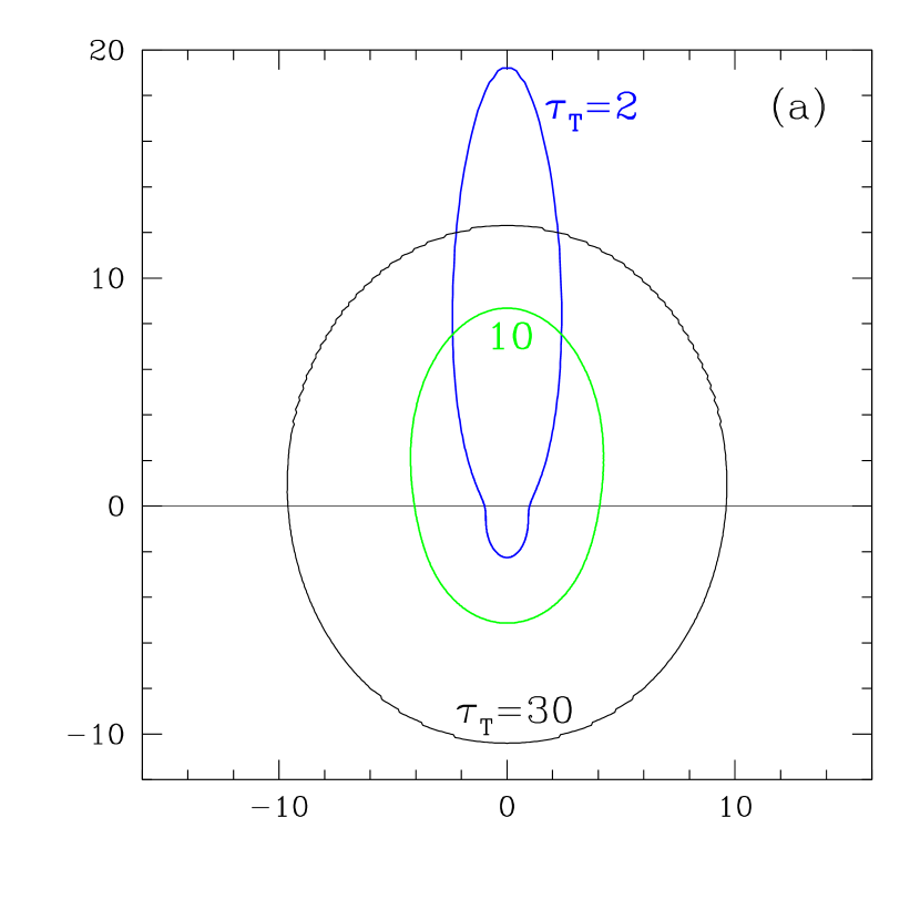
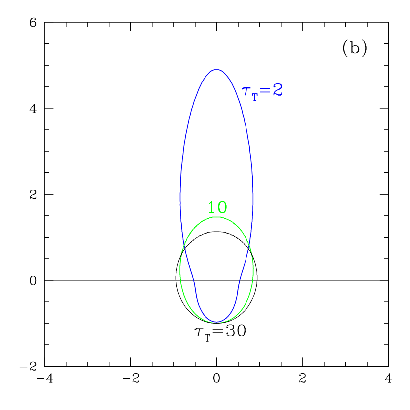
Figure 5.— (a) Same as Fig. 1 but for Thomson scattering and taking into account polarization. The plot shows intensity $I(\mu)$ (in the fluid frame) at three radii: $r/R_{\star}\approx 0.03$, $0.1$ and $0.5$. (b) The corresponding solution for the photon-number intensity ${\cal I}(\mu)$. It is normalized so that ${\cal I}_{1}+\beta{\cal I}_{0}=1$ (note that ${\cal I}_{1}[r]+\beta{\cal I}_{0}[r]=const$ expresses conservation of photon number, see Section 2.3); $\beta=1$ in our transfer problem.

Figure 6.— Polarization degree of radiation transferred through the outflow with Thomson scattering opacity, $p=Q/I$. Dashed curve shows the polarization of radiation propagating at angle $\theta=\pi/2$ in the fluid frame. Solid curve shows the angle-averaged polarization defined in equation (22).

Similar to Section 3, we will consider here outflows with $\dot{N}_{e}(r)=const$ and $\Gamma(r)=const$. This implies $\tau_{\rm T}(r)=R_{\star}/r$ and $g=1$. Equations (17) and (18) are solved numerically in the same way as described in Section 3.1. The resulting angular distribution of intensity $I$ in the fluid frame is shown in Figure 5a. It is similar to the model with isotropic scattering (Fig. 1).

The polarization degree of radiation is shown in Figure 6. It begins to grow in the subphotospheric region (where anisotropy develops), and radiation becomes significantly polarized in the photospheric region. The strongest polarization $p\approx 0.6$ is found at large radii for radiation at angles $\theta\approx\pi/2$. It is produced by scattering of strongly beamed radiation, which naturally generates a high polarization at scattering angles close to 90 degrees. The overall polarization at a given radius may be described by the average $p$ that is defined using the energy fluxes in the two modes measured in the lab frame. This definition involves the transformation of moments $I_{m}$ and $Q_{m}$ to the lab frame, which gives

$$<p>=\frac{\tilde{Q}_{1}}{\tilde{I}_{1}}=\frac{\beta(Q_{0}+Q_{2})+(1+\beta^{2})Q_{1}}{\beta(I_{0}+I_{2})+(1+\beta^{2})I_{1}}.$$ (22)

This expression is well-behaved in the limit $\beta\rightarrow 1$ and becomes $<p>=(Q_{0}+2Q_{1}+Q_{2})/(I_{0}+2I_{1}+I_{2})$. It reaches 0.24 outside the photosphere (Fig. 6).

Equations (17) and (18) govern the transfer of energy in the two polarization modes. The photon number in the two modes is described by intensities ${\cal I}_{\perp}$ and ${\cal I}_{\parallel}$. The equations for ${\cal I}={\cal I}_{\perp}+{\cal I}_{\parallel}$ and ${\cal Q}={\cal I}_{\perp}-{\cal I}_{\parallel}$ read (cf. the similar eq. 10)

$$\frac{\partial{\cal I}}{\partial\ln r}=-\left(1-\mu^{2}\right)\,g\,\frac{\partial{\cal I}}{\partial\mu}-3\,(1-\mu g)\,{\cal I}+\tau_{\rm T}\,\frac{({\cal S}-{\cal I})}{1+\mu},$$ (23)

$$\frac{\partial{\cal Q}}{\partial\ln r}=-\left(1-\mu^{2}\right)\,g\,\frac{\partial{\cal Q}}{\partial\mu}-3\,(1-\mu g)\,{\cal Q}+\tau_{\rm T}\,\frac{({\cal R}-{\cal Q})}{1+\mu}.$$ (24)

The source functions ${\cal S}$ and ${\cal R}$ are related to the moments ${\cal I}_{m}$ and ${\cal Q}_{m}$ ($m=0,1,2$) in the same way as $S$ and $R$ are related to $I_{m}$ and $Q_{m}$ (eqs. 19 and 20).

We numerically solved equations (23) and (24) with $g=1$. The resulting angular distribution ${\cal I}(\mu,r)$ is shown in Figure 5b. It is less anisotropic than the energy intensity $I(\mu,r)$. (A similar result is found in the isotropic-scattering model.) Correspondingly, the quantity ${\cal Q}/{\cal I}$ is smaller than $p=Q/I$, roughly by a factor of $\sim 3/4$.

Figure 7.— Comparison of photon-number intensity ${\cal I}(\mu)$ at $r=R_{\star}/2$ in three models: isotropic coherent scattering (dashed curve), polarized Thomson scattering in a cold outflow (solid curve), and unpolarized Compton scattering in a hot outflow (open circles), see text for the description of the hot-outflow model. In all three models, the intensity is normalized so that the conserved quantity ${\cal I}_{1}+\beta{\cal I}_{0}$ equals unity. The models assume $\beta\approx 1$.

4.2. Scattering in a hot plasma

GRB jets are heated, which leads to Comptonization — a significant flow of heat from particles to radiation. This process depends on the electron temperature that must be calculated self-consistently. For example, consider the fiducial model of the collisionally-heated jet in B10. The jet with Lorentz factor $\Gamma=600$ is heated at radii $r>R_{n}\approx R_{\star}/20$, and its electron temperature outside $R_{n}$ may be approximated by

$$\Theta_{e}\equiv\frac{kT_{e}}{m_{e}c^{2}}=0.045\,\left(\frac{r}{R_{\star}}\right)^{0.23}.$$ (25)

The initial temperature of radiation at $R_{n}$ is 0.6 keV. Comptonization begins at $R_{n}$ with Kompaneets’ $y$-parameter $y=4\Theta_{e}\tau_{\rm T}\sim 1$. Equation (25) is a reasonable approximation in the main heating region $R_{\star}/20<r<R_{\star}$. The exact value of temperature outside $R_{\star}$ is not important — its contribution to thermal Comptonization is small, — and the above approximation for $T_{e}$ will be sufficient for our purposes.

Comptonization significantly changes the energy intensity $I(\mu,r)$ compared with the cold-jet model. In addition to the thermal plasma, nonthermal particles are continually injected with energies $\sim 140$ MeV from the decay of pions produced by nuclear collisions. These particles convert their energy to a small number of high-energy photons, which impact the radiative transfer and the observed spectrum above 20 MeV (B10).

Here, however, we limit our consideration to the transfer of photon number (rather than energy). The high-energy photons make a negligible contribution to the number intensity ${\cal I}(\mu,r)$, so it is sufficient to consider scattering by the thermal plasma with temperature (25), which strongly dominates the optical depth. The solution for the number intensity ${\cal I}(\mu,r)$ turns out to be close to that in a cold jet. The obtained angular distribution of Comptonized photons at $r=R_{\star}/2$ is shown by open circles in Figure 7. Its beaming is somewhat stronger compared with the cold-jet model of Section 4.1, however the difference is modest. The effect of electron heating on the transfer solution for photon number is $\sim 10$%.

5. Radiation-dominated outflow

Anisotropic radiation always tends to push the flow toward the equilibrium velocity at which the net flux of radiation vanishes in the fluid frame. When this effect is strong, it leads to the peculiar “equilibrium transfer” where radiation and plasma self-organize to flow with a common velocity (Beloborodov 1998, 1999). In this section, we discuss the conditions for this regime and the corresponding solution of the transfer problem.

The radiative force applied to each electron (or positron) in the fluid frame is given by $f=4\pi I_{1}\sigma_{\rm T}/c$. We assume that the electron thermal motion in the fluid frame is slow (non-relativistic). Then Lorentz transformation gives the same value for the force measured in the lab frame, $\tilde{f}=f$. The outflow acceleration is governed by the dynamic equation,

$$\frac{\rho}{n}\,c^{2}\beta\,\frac{d(\Gamma\beta)}{dr}=4\pi I_{1}\,\frac{\sigma_{\rm T}}{c}.$$ (26)

Here $I_{1}$ is the first moment of radiation in the fluid frame (eq. 7), $\rho$ is the rest-mass density of the plasma, and $n$ is the number density of $e^{\pm}$; both $\rho$ and $n$ are measured in the fluid frame. Then, for ultra-relativistic outflows ($\beta\rightarrow 1$), one finds

$$g=1-\frac{d\ln\Gamma}{d\ln r}=1-\frac{4\pi I_{1}}{\rho c^{3}}\,\tau_{\rm T}.$$ (27)

One can use the approximation $g=1$ (i.e. $\Gamma=const$) if the last term in equation (27) is much smaller than unity. At the photospheric radius $R_{\star}$ this term equals $4\pi I_{1}\,(\rho c^{3})^{-1}=\chi\,(U/\rho c^{2})$ where $\chi=I_{1}/I_{0}<1$ is a numerical factor that depends on the angular distribution of radiation and $U=4\pi I_{0}/c$ is the radiation energy density in the fluid frame. If $U/\rho c^{2}$ is not small compared with unity, the transfer equation should be solved with the self-consistent function $g(r)$ given by equation (27).

The self-consistent solution of the transfer problem can be obtained analytically in the extreme radiation-dominated regime $U/\rho c^{2}\gg 1$. Note that there exists a special value of $\Gamma=\Gamma_{0}$ for which the radiative force (eq. 26) vanishes; this value corresponds to $I_{1}=0$. The force is positive if $\Gamma<\Gamma_{0}$ and negative if $\Gamma>\Gamma_{0}$, i.e. it always pushes the outflow toward $\Gamma=\Gamma_{0}$. In the radiation-dominated regime, the timescale for dynamical relaxation toward $\Gamma=\Gamma_{0}$ is shorter than the outflow expansion timescale. This means that the outflow maintains $\Gamma\approx\Gamma_{0}$ and $I_{1}\ll I_{0}$.

In this regime, the ultra-relativistic transfer has a simple solution,

$$I(\mu,r)=\frac{C}{r^{4}},\qquad Q(\mu,r)=0,\qquad g=0,$$ (28)

where $C$ is a constant determined by the inner boundary condition. It is straightforward to verify that equation (28) is the solution of equations (17) and (18). The first moment $I_{1}$ is a small (next-order) quantity. It controls the outflow acceleration $\Gamma\propto r$ and is given by $I_{1}=(4\pi\tau_{\rm T})^{-1}\rho c^{3}\ll I_{0}$. The outflow accelerates linearly with radius both inside and outside the photosphere, as long as $U\gg\rho c^{2}$. Note that $U/\rho c^{2}\propto r^{-1}$, so the outflow eventually must reach radii where $U<\rho c^{2}$ and the acceleration ends. This transition occurs outside $R_{\star}$ and has no effect on radiation escaping the outflow to distant observers.

Equation (28) states that radiation remains isotropic in the fluid frame which accelerates as $\Gamma\propto r$. The sustained isotropy is a consequence of a remarkable fact: a freely propagating photon between two successive scatterings at radii $r_{1}$ and $r_{2}$ does not change its angle measured in the fluid frame, $\theta_{1}=\theta_{2}$. This fact can be derived as follows. In the lab frame the angle of a photon propagating from $r_{1}$ to $r_{2}$ satisfies the equation of a straight line, $r_{1}\sin\tilde{\theta}_{1}=r_{2}\sin\tilde{\theta}_{2}$. Using $r_{2}/r_{1}=\Gamma_{2}/\Gamma_{1}$ and Doppler transformation $\sin\theta={\cal D}\sin\tilde{\theta}$ (where ${\cal D}=\Gamma[1+\cos\theta]$ when $\beta\rightarrow 1$), one finds $\theta_{1}=\theta_{2}$.

Thus, free propagation between scatterings does not generate any change in the angular distribution of photons in the fluid frame, and an initially isotropic radiation remains isotropic, $I=I_{0}$. Scattering of isotropic radiation gives isotropic radiation, so the source function also remains isotropic in the fluid frame, $S=I_{0}$. Naturally, the isotropic radiation remains unpolarized.

It is easy to see why the energy intensity in the fluid frame scales with radius as $I\propto r^{-4}$. First note that conservation of photon number implies that the photon-number intensity scales as ${\cal I}\propto\Gamma^{-1}r^{-2}\propto r^{-3}$ (see Section 2.3 and use isotropy, ${\cal I}\approx{\cal I}_{0}$ and ${\cal I}_{1}\ll{\cal I}_{0}$). Coherent scattering does not affect the photon energy in the fluid frame, so $\nu$ changes only during free propagation of the photon. Propagation between successive scatterings at $r_{1}$ and $r_{2}$ occurs with constant energy in the lab frame, ${\cal D}_{2}\,h\nu_{2}={\cal D}_{1}\,h\nu_{1}$. Using $\theta_{2}=\theta_{1}$, one finds $\nu_{2}/\nu_{1}={\cal D}_{2}/{\cal D}_{1}=\Gamma_{2}/\Gamma_{1}=r_{2}/r_{1}$. Thus, $\nu\propto r^{-1}$ for each photon. Together with ${\cal I}\propto r^{-3}$ this implies $I\propto r^{-4}$.

The existence of a frame (fluid frame) where radiation remains isotropic and scattering is coherent implies that scattering has no effect on radiation, i.e. the transfer occurs as if radiation propagated in vacuum. Indeed, consider the basic transfer equation (A1) in the lab frame. Coherent isotropic scattering in the fluid frame gives $S_{\nu}=I_{\nu}$, which implies $\tilde{S}_{\nu}=\tilde{I}_{\nu}$ in the lab frame and hence $d\tilde{I}_{\nu}/ds=0$. Thus, radiation intensity in the lab frame remains constant along the ray, just like propagation in vacuum. In particular, the spectrum of radiation is preserved and its beaming angle decreases as $r^{-1}$.

The corresponding solution for the intensity in the fluid frame can be obtained by the Doppler transformation $I_{\nu}={\cal D}^{-3}\tilde{I}_{\nu}$ (Appendix A) of the vacuum solution for $\tilde{I}_{\nu}$. Alternatively, the same result can be obtained from equation (1). Substituting $g=0$, one gets

$$I_{\nu}(\nu,\mu,r)=I_{\nu}\left(\frac{\nu\,r}{r_{\rm in}},\mu,r_{\rm in}\right)\,\left(\frac{r}{r_{\rm in}}\right)^{-3}.$$ (29)

It confirms that, when viewed in the fluid frame, the transfer preserves isotropy of photon distribution and shifts each photon in frequency as $r^{-1}$.

To summarize, as long as $U\gg\rho c^{2}$ radiation behaves as if there were no scattering and it streamed freely, regardless of the optical depth. This is a special feature of the ultra-relativistic transfer in spherical geometry. It differs from the radiation-dominated transfer with $\Gamma=\Gamma_{0}$ in the plane-parallel geometry (Beloborodov 1998; 1999).

6. Variable jets and the steady spherically symmetric model

In this paper, we considered radiative transfer in outflows that are steady and spherically symmetric. Here we discuss why these assumptions are not so restrictive as they might seem and the model may describe variable jets.

Radial outflows with Lorentz factors $\Gamma\gg 1$ have two well-known features: (1) Their parts are causally disconnected on scales larger than $l_{\perp}\sim r/\Gamma$ on any sphere of radius $r$ ($r\sim R_{\star}$ should be taken as the characteristic radius for the problem of photospheric emission). (2) Since both radiation and fluid move outward with almost speed of light, the radial diffusion of radiation relative to the fluid is inefficient on scales $\delta r\gg l_{\parallel}$ where $l_{\parallel}\sim r/\Gamma^{2}$. To a first approximation, each “elementary pancake” of volume $l_{\parallel}\times l_{\perp}\times l_{\perp}$ in the lab frame has its own radiative transfer and produces photospheric emission almost independently from the neighboring pancakes. If strong inhomogeneities of the jet are confined to scales much larger than $l_{\parallel}$ and $l_{\perp}$ (in the radial and transverse directions, respectively), radiative transfer in each pancake occurs as if it were part of a steady, spherically symmetric outflow.

The independence of emissions from different pancakes can be better quantified if one considers the photon exchange between two pancakes separated by $\delta r>l_{\parallel}$. The exchange is one-way only: the trailing pancake can receive photons from the leading pancake (the opposite communication is impossible for $\delta r>l_{\parallel}$). This “trailing diffusion” of radiation was studied by Pe’er (2008). He considered a very narrow shell of photons (formally a delta-function of radius) injected at a small $r$ in a steady jet with a constant Lorentz factor. The photons diffuse through the jet and eventually escape, producing an isolated pulse of emission that will be received by a distant observer. The characteristic observed width of this pulse is $\delta t_{\rm obs}\sim t_{\star}=l_{\parallel}/c\sim R_{\star}/\Gamma^{2}c$, and it has an extended tail whose intensity decreases as $(t_{\rm obs}/t_{\star})^{-2}$. This implies that the trailing diffusion of radiation on scales $\delta r>l_{\parallel}$ is suppressed as $(\delta r/l_{\parallel})^{-2}$.

A realistic GRB jet is continually filled with thermal radiation near the central engine. It may be viewed as a continual sequence of elementary pancakes that release their photons near $R_{\star}$. The strong Doppler beaming implies that photospheric emission seen by a distant observer is dominated by a small patch $l_{\perp}\times l_{\perp}$ on the sphere of radius $\sim R_{\star}$. The observer receives radiation released by consecutive pancakes in the same order as they pass through $R_{\star}$. The observed timescale of passage of one elementary pancake through $R_{\star}$ is $t_{\star}$, which may be smaller than 1 ms for GRBs. The steady transfer model developed in this paper is valid for GRBs with variability timescales $\delta t_{\rm obs}>t_{\star}$. The model permits different $R_{\star}$ for pancakes separated by timescales $\delta t_{\rm obs}=\delta r/c\gg t_{\star}$.

7. Discussion

This paper explored radiative transfer in ultra-relativistic outflows. The transfer problem is well defined and simplifies in the limit $\Gamma\gg 1$. In this limit, radiation propagating backward in the lab frame can be neglected. Therefore, the transfer solution is independent of the outer boundary condition, in contrast to transfer in static media studied by Chandrasekhar (1960) and Sobolev (1963). The problem is solved by direct integration of the transfer equation, with no need for iterations. The model with $\Gamma\rightarrow\infty$ gives excellent approximation to transfer in outflows with finite $\Gamma>10$.

7.1. Transfer in radiation-dominated and matter-dominated outflows

The approach developed in this paper gives a simple solution for the old problem of radiation-dominated jet discussed by Paczyński (1986) and Goodman (1986). This jet is baryon-clean. It is very opaque at small radii because of the thermal population of $e^{\pm}$ pairs. Almost all pairs annihilate at larger radii, and almost all the jet energy is carried by radiation that is released at the photosphere. Paczyński and Goodman considered the opaque zone of the radiation-dominated jet and derived its Lorentz factor $\Gamma\propto r$ from energy-momentum conservation. They argued that quasi-thermal emission should be observed from the jet, with a spectral peak near 1 MeV. They suggested, however, that the observed spectrum should be different from blackbody because of complicated transfer effects near the photosphere. Goodman (1986) performed a numerical calculation with simplifying assumptions, which gave a nonblackbody spectrum.

In fact, the exact transfer solution for this problem gives precisely blackbody spectrum. As shown in Section 5, photons in a radiation-dominated jet are transferred as if there were no scattering at all. The radiation remains isotropic in the fluid frame which accelerates as $\Gamma\propto r$ both inside and outside the photosphere. A distant observer can think that radiation freely propagates from the central engine of the jet. Note also that regardless of how strong dissipation/heating may occur in the jet it does not have a dramatic impact on the shape of the spectral peak, because the energy budget of heating is negligible compared with the Planck radiation. The observed radiation should have a blackbody spectrum.

The opposite, “matter-dominated” regime was considered by Paczyński (1990). In the opaque zone radiation cools adiabatically and the jet energy becomes dominated by baryons. Then it continues inertial expansion (coasting) with some relict thermal radiation in it until the radiation is released at the photosphere.

In the matter-dominated regime, the photospheric spectrum cannot have the blackbody shape, even if the outflow cools passively, with no heating, up to the photosphere. B10 showed that the photospheric spectrum in the soft X-ray band has the slope $\alpha\approx 0.4$ instead of the blackbody (Rayleigh-Jeans) slope $\alpha=1$. Moreover, collisional heating in GRB jets transforms the photospheric spectrum into the Band-type radiation, with extended high-energy emission instead of the exponential cutoff above 1 MeV. Thus, the photospheric spectrum of a matter-dominated jet is changed from blackbody both below and above the MeV peak.

Besides giving a non-blackbody spectrum, the radiative transfer in matter-dominated jets has other interesting features. Radiation becomes strongly anisotropic in the fluid frame well before it decouples from the fluid. Radiation at the characteristic photospheric radius $R_{\star}$ has the beaming factor $b\sim 30$ (Fig. 2). Beaming affects the adiabatic cooling of photons in the subphotospheric region. The net cooling factor for radiation emitted at a radius $r_{\rm in}\ll R_{\star}$ equals $2(r_{\rm in}/R_{\star})^{2/3}$.

In a heated jet, adiabatic cooling of radiation is counter-balanced (or dominated) by Comptonization, so the mean photon energy can grow with radius. This has a strong effect on the transfer solution for the radiation intensity. However, if one focuses on the transfer of photon number (rather than energy), the results are not sensitive to heating. The photon-number intensity ${\cal I}$ in the passively cooling and heated jets is very similar (the difference is $\sim 10$%). In both cases, ${\cal I}$ is strongly beamed in the subphotospheric region (Fig. 7).

7.2. Detecting the blackbody component in GRBs

As discussed in Section 7.1, photospheric emission in GRBs can have a blackbody spectrum only when the photosphere is dominated by radiation (i.e. $U\gg\rho c^{2}$ at $r\sim R_{\star}$). The detection of a blackbody component in a GRB spectrum would provide clear evidence that part of the photospheric emission is in the radiation-dominated regime.

The existing data are inconclusive. It includes GRB 090902B that was much discussed recently as a burst with a blackbody component. In fact, it is equally well fitted by the Band function plus a power law (Ryde et al. 2010). The data interpretation is further complicated by the variability of photospheric emission. It may vary on very short timescales, as short as $t_{\star}\sim R_{\star}/c\Gamma^{2}$, which can be smaller than one millisecond for a typical GRB. The achieved temporal resolution of spectral analysis is far worse than 1 ms and may not give the true instantaneous photospheric spectrum. The photospheric emission may quickly switch between the radiation-dominated and matter-dominated regimes and these variations would remain undetected.

The low-energy slopes of the observed GRB spectra, $\alpha$, are affected by the time averaging, which tends to reduce $\alpha$. Bursts with largest $\alpha$ are most promising for detecting the blackbody component. In some cases, $\alpha\sim 1$ were reported (Ghirlanda, Celotti & Ghisellini 2003). This indicates the existence of the radiation-dominated regime.

7.3. Detecting photospheric polarization

Radiation remains unpolarized in radiation-dominated jets (Section 5). In contrast, in matter-dominated jets, radiation acquires a strong linear polarization in the photospheric region (Section 4.1). An ideal detector that has enough angular resolution to image the spherically-symmetric outflow on scales $\sim\Gamma^{-1}R_{\star}$ would detect the polarization. In practice, such a high angular resolution is not achieved. The detectors receive a mixture of radiation whose polarization averages to zero unless something breaks spherical symmetry.

Three principle possibilities for breaking the symmetry are as follows: (1) The main emitting region of size $l_{\perp}\sim\Gamma^{-1}R_{\star}$ is partially eclipsed. (2) The outflow deviates from spherical symmetry on scales $\sim l_{\perp}$. (3) The jet carries magnetic fields with a coherence scale $\mathrel{\hbox{\raise 2.15277pt\hbox{$>$}\hbox to0.0pt{\hss\lower 2.15277pt\hbox{$\sim$}}}}l_{\perp}$. In magnetized jets, the synchrotron component of photospheric emission becomes dominant at photon energies below $\sim 100$ keV (B10; Vurm et al. 2011). This component can be highly polarized. Future polarization measurements across the X-ray spectrum will help estimate the magnetization of GRB jets.

7.4. Modeling frequency-dependent radiative transfer in heated jets

The photosphere of a baryonic jet is a fuzzy object — about 2/3 of photons are released in the region $R_{\star}/3<r<3R_{\star}$, and the remaining 1/3 comes from even more extended region. Modeling the heated anisotropic radiation emerging from this region requires accurate transfer simulations.

B10 developed a Monte-Carlo transfer code that solves the transfer problem in a broad range of photon energies up to 100 GeV, including the effects of $\gamma$-$\gamma$ absorption. Alternatively, one can use the kinetic method that solves the kinetic equations for the photon and electron distribution functions (Pe’er & Waxman 2005; Vurm & Poutanen 2009). The developed kinetic codes have, however, one drawback: they assume isotropic radiation in the fluid frame, which is not a good approximation. Besides, it violates conservation of photon number in the lab frame. The kinetic method can be used more efficiently if it calculates the evolution of radiation by solving the transfer equation (1). This method will be implemented in an upcoming paper (Vurm et al. 2011).

Appendix A A. Basic equations of relativistic transfer

Consider radiation with specific intensity $\tilde{I}_{\nu}(\tilde{\nu},\tilde{\mu},r)$ in the fixed lab frame. Here $\tilde{\nu}$ is the photon frequency, $\tilde{\mu}=\cos\tilde{\theta}$, and $\tilde{\theta}$ is the photon angle with respect to the radial direction. Hereafter quantities measured in the fixed lab frame are denoted with tilde. The transfer equation reads

$$\frac{d\tilde{I}_{\nu}}{ds}=\tilde{\kappa}_{\nu}(\tilde{S}_{\nu}-\tilde{I}_{\nu}),$$ (A1)

where $ds$ is the path element along the ray and $\tilde{\kappa}_{\nu}(\tilde{\nu},\tilde{\mu},r)$ is the absorption coefficient of the outflow in the lab frame. The source function $\tilde{S}_{\nu}$ equals $\tilde{j}_{\nu}/\tilde{\kappa}_{\nu}$, the ratio of emission and absorption coefficients (e.g. Chandrasekhar 1960).

The outflow in our problem is moving radially with velocity $\beta(r)$ and Lorentz factor $\Gamma(r)$. The transfer equation in the lab frame is not well behaved in the ultra-relativistic limit $\Gamma\gg 1$. Therefore, we rewrite it in terms of intensity $I_{\nu}$ measured in the fluid frame, i.e. in the frame comoving with the outflow. This is straightforward to do using the usual transformation laws (Prokof’ev 1962; Castor 1972; Mihalas 1980). The transformations are given by

$$\tilde{I}_{\nu}={\cal D}^{3}I_{\nu},\qquad\tilde{S}_{\nu}={\cal D}^{3}S_{\nu},$$ (A2)

$$\tilde{\nu}={\cal D}\nu,\qquad{\cal D}=\Gamma(1-\beta\tilde{\mu})^{-1}=\Gamma(1+\beta\mu),$$ (A3)

$$\tilde{\mu}=\frac{\mu+\beta}{1+\beta\mu}.$$ (A4)

$$\tilde{\kappa}_{\nu}={\cal D}^{-1}\kappa_{\nu}.$$ (A5)

Using $\tilde{I}_{\nu}/\tilde{\nu}^{3}=I_{\nu}/\nu^{3}$ and $\tilde{S}_{\nu}/\tilde{\nu}^{3}=S_{\nu}/\nu^{3}$, equation (A1) may be written as

$$\nu^{3}\,\frac{d}{ds}\left(\frac{I_{\nu}}{\nu^{3}}\right)=\frac{\kappa_{\nu}}{{\cal D}}\left(S_{\nu}-I_{\nu}\right).$$ (A6)

$I_{\nu}$ is considered as a function of $r$, $\mu$, $\nu$, and the derivative along the ray is expanded as

$$\frac{dI_{\nu}}{ds}=\frac{dr}{ds}\,\frac{\partial I_{\nu}}{\partial r}+\frac{d\mu}{ds}\,\frac{\partial I_{\nu}}{\partial\mu}+\frac{d\ln\nu}{ds}\,\frac{\partial I_{\nu}}{\partial\ln\nu}.$$ (A7)

Here one can use $dr/ds=\tilde{\mu}$, $d\tilde{\nu}/ds=0$, and $d\tilde{\mu}/ds=(1-\tilde{\mu}^{2})/r$ (a consequence of $r\sin\tilde{\theta}=const$, which is valid for any straight line). The corresponding derivatives of $\nu$ and $\mu$ are obtained using the transformations (A3) and (A4). This gives

$$\frac{dr}{ds} = \frac{\Gamma}{{\cal D}}\,(\mu+\beta),$$ (A8)

$$\frac{d\mu}{ds} = \frac{1-\mu^{2}}{r}\left[1-\frac{\Gamma}{{\cal D}\beta}\,(\mu+\beta)\,\frac{d\ln\Gamma}{d\ln r}\right],$$ (A9)

$$\frac{d\ln\nu}{ds} = -\frac{\Gamma\beta}{{\cal D}}\,\frac{(1-\mu^{2})}{r}-\frac{\Gamma\,\mu}{{\cal D}\beta}\,(\mu+\beta)\,\frac{d\ln\Gamma}{dr},$$ (A10)

where we used $d\beta=d\Gamma/\beta\Gamma^{3}$ and $(1-\tilde{\mu}^{2})={\cal D}^{-2}(1-\mu^{2})$. Then equation (A6) becomes,

$$(\mu+\beta)\,\frac{\partial I_{\nu}}{\partial\ln r}+\left(1-\mu^{2}\right)\left[1+\beta\mu-\frac{(\mu+\beta)}{\beta}\,\frac{d\ln\Gamma}{d\ln r}\right]\,\frac{\partial I_{\nu}}{\partial\mu}-\left[\beta\left(1-\mu^{2}\right)+\frac{\mu(\mu+\beta)}{\beta}\,\frac{d\ln\Gamma}{d\ln r}\right]\left(\frac{\partial I_{\nu}}{\partial\ln\nu}-3I_{\nu}\right)=\tau_{\nu}(S_{\nu}-I_{\nu}),$$ (A11)

where

$$\tau_{\nu}(r,\nu)\equiv\frac{\kappa_{\nu}(r,\nu)\,r}{\Gamma}.$$ (A12)

Equation (2.12) in Mihalas (1980) is reduced to equation (A11) in the steady case.

Appendix B B. Analytic solution

In Section 2 we solved the transfer equation numerically. Here we collect useful analytical formulas that may be used instead of the numerical solution.

B.1. Optical depth along the ray

Consider a photon propagating from radius $r_{1}$ to $r_{2}$ along a straight line in the lab frame. Let $\tilde{\theta}_{1}$ be photon angle at $r_{1}$. The optical depth along the ray from $r_{1}$ to $r_{2}$ is

$$\tau_{\rm ray}(r_{1},\tilde{\theta}_{1},r_{2})=\int_{r_{1}}^{r_{2}}\tilde{\kappa}(r,\tilde{\theta})\,\frac{dr}{\cos\tilde{\theta}}.$$ (B1)

Here $\tilde{\theta}(r)$ is photon angle at radius $r$. It satisfies the relation (which expresses the fact the photon moves along a straight line),

$$r\sin\tilde{\theta}=r_{1}\sin\tilde{\theta}_{1}.$$ (B2)

The scattering opacity in the lab frame is given by $\tilde{\kappa}={\cal D}^{-1}\kappa=\Gamma(1-\beta\cos\tilde{\theta})\,\sigma n$. Let us consider an outflow with $\Gamma(r)=const$ and $n\propto r^{-2}$. Then the elementary integral in equation (B1) gives

$$\tau_{\rm ray}(r_{1},\tilde{\theta}_{1},r_{2})=\tau(r_{1})\,\Gamma^{2}\left[\frac{\tilde{\theta}_{1}-\tilde{\theta}_{2}}{\sin\tilde{\theta}_{1}}-\beta\left(1-\frac{r_{1}}{r_{2}}\right)\right],$$ (B3)

where $\tau(r)\equiv n\sigma r/\Gamma$. If $\Gamma\gg 1$, one can expand equation (B3) in $\Gamma^{-1}$,

$$\tau_{\rm ray}(r_{1},x_{1},r_{2})=\frac{\tau(r_{1})}{6}\left(1-\frac{r_{1}}{r_{2}}\right)\left[3+\left(1+\frac{r_{1}}{r_{2}}+\frac{r_{1}^{2}}{r_{2}^{2}}\right)\,x_{1}\right]+{\cal O}\left(\Gamma^{-2}\right).$$ (B4)

Here $x={\cal O}(1)$ is a convenient variable related to the photon angle,

$$x\equiv\Gamma^{2}\tilde{\theta}^{2}=\frac{1-\mu}{1+\mu},$$ (B5)

where $\mu=\cos\theta$ is measured in the fluid frame.

If we take $r_{2}\rightarrow\infty$ and drop index “1” for the emission point, equations (B3) and (B4) are reduced to

$$\tau_{\rm ray}(r,x,\infty)=\tau(r)\,\Gamma^{2}\left(\frac{\tilde{\theta}}{\sin\tilde{\theta}}-\beta\right)=\frac{\tau(r)}{6}\left(3+x\right)+{\cal O}\left(\Gamma^{-2}\right).$$ (B6)

A similar formula for the optical depth along the ray from radius $r$ to infinity is given in Abramowicz et al. (1991) and Pe’er (2008).

B.2. Expressions for intensity and source function

The formal solution for the transfer problem is written in terms of the source function. Let us first consider the transfer of photon number (Section 2.3). The corresponding intensity in the lab frame is given by

$$\tilde{\cal I}(\tilde{\mu},r)=\int_{0}^{\infty}\tilde{\cal S}(\tilde{\mu}_{1},r_{1})\,\exp\left[-\tau_{\rm ray}(r_{1},\tilde{\mu}_{1},r)\right]\,d\tau_{\rm ray}(r_{1},\tilde{\mu}_{1},r),$$ (B7)

where $r_{1}<r$ is running along the ray and $\tilde{\mu}_{1}=\cos\tilde{\theta}_{1}$ is related to $\tilde{\mu}=\cos\tilde{\theta}$ by equation (B2). Equation (B7) can be rewritten in terms of ${\cal I}(\mu,r)$ and ${\cal S}(\mu,r)$ using the transformations $\tilde{\cal I}={\cal D}^{3}{\cal I}$ and $\tilde{\cal S}={\cal D}^{3}{\cal S}$. For outflows with $\beta\rightarrow 1$ this gives

$${\cal I}(\mu,r)=\int_{0}^{\infty}{\cal S}(\mu_{1},r_{1})\,\left(\frac{1+\mu_{1}}{1+\mu}\right)^{3}\exp\left[-\tau_{\rm ray}(r_{1},\mu_{1},r)\right]\,d\tau_{\rm ray}(r_{1},\mu_{1},r).$$ (B8)

Here one can substitute equation (B4) for $\tau_{\rm ray}(r_{1},\mu_{1},r)$. The identity $\tau_{\rm ray}(r_{1},\mu_{1},r)=-\tau_{\rm ray}(r,\mu,r_{1})$ simplifies the integral.

It is sufficient to know the source function ${\cal S}(\mu,r)$ to reconstruct the solution for ${\cal I}(\mu,r)$. In the model with isotropic scattering the source function ${\cal S}={\cal I}_{0}(r)$ does not depend on $\mu$. Our numerical result for ${\cal I}_{0}(r)$ agrees within a few percent with the following formula,

$$r^{2}\,{\cal I}_{0}(r)={\cal K}\,\left\{\frac{3}{2}+\frac{1}{\pi}\arctan\left[\frac{1}{3}\left(\frac{R_{\star}}{r}-\frac{r}{R_{\star}}\right)\right]\right\},$$ (B9)

where ${\cal K}$ is a constant. It can be expressed in terms of the photon flux in the lab frame $\tilde{\cal F}$ (Section 2.3), which satisfies $r^{2}\tilde{\cal F}(r)=const$. At $r/R_{\star}\gg 1$ we have ${\cal I}_{1}={\cal I}_{0}$ and $\tilde{\cal F}=4\pi\Gamma(1+\beta){\cal I}_{0}$. This gives (with $\beta\rightarrow 1$)

$${\cal K}=\frac{r^{2}\tilde{\cal F}(r)}{8\pi\Gamma}.$$ (B10)

Substitution of equation (B9) to equation (B8) and its integration over radius recovers ${\cal I}(\mu,r)$ that was found by direct numerical integration of the transfer equation.

Similarly, the formal solution for transfer of energy is given by

$$I(\mu,r)=\int_{0}^{\infty}S(\mu_{1},r_{1})\,\left(\frac{1+\mu_{1}}{1+\mu}\right)^{4}\exp\left[-\tau_{\rm ray}(r_{1},\mu_{1},r)\right]\,d\tau_{\rm ray}(r_{1},\mu_{1},r).$$ (B11)

The model with isotropic coherent scattering has $S(\mu,r)=I_{0}(r)$. In this case, one can use the following formula,

$$r^{2}\,I_{0}(r)=K\,\left(\frac{1}{2}+\frac{R_{\star}}{r}\right)^{2/3},$$ (B12)

where constant $K$ is determined by the inner boundary condition at $r\ll R_{\star}$. Equation (B12) remains approximately valid for cold outflows with Thomson scattering. For heated jets with significant Comptonization of radiation, $I_{0}(r)$ and $S(\mu,r)$ are different and depend on the heating history.

In contrast, equation (B9) remains an excellent approximation even for heated outflows, as long as scattering is the main source of opacity and emissivity.

B.3. Distribution of the last-scattering radius and angle

Consider all photons escaping to infinity from a steady, spherically symmetric outflow. Let $\dot{N}$ be the number of escaping photons per unit time, measured in the lab frame. One can think of $\dot{N}$ as the rate of photon emission by a source distributed throughout the volume of the outflow and attenuated by the optical depth. The photon emission rate from volume element $dV$ into solid angle $d\tilde{\Omega}$ is $\tilde{\epsilon}\,dV\,d\tilde{\Omega}$, where $\tilde{\epsilon}(r_{\star},\tilde{\theta}_{\star})$ is the photon emissivity in the lab frame. It depends on the radial position of the emitter $dV$, $r_{\star}$, and the emission angle with respect to the radial direction, $\tilde{\theta}_{\star}$. The attenuation factor is $\exp[-\tau_{\rm ray}(r_{\star},\tilde{\theta}_{\star},\infty)]$, which gives

$$\frac{d\dot{N}}{dV\,d\tilde{\Omega}}=\tilde{\epsilon}\,\exp\left[-\tau_{\rm ray}(r_{\star},\tilde{\theta}_{\star},\infty)\right].$$ (B13)

A similar expression holds for the angular distribution measured in the fluid frame (note that $\tilde{\epsilon}\,d\tilde{\Omega}={\epsilon}\,d\Omega$ is invariant under Lorentz transformation). Substituting $dV=4\pi r_{\star}^{2}\,dr_{\star}$, $d\Omega=d\phi_{\star}\,d\mu_{\star}$ (where $\mu_{\star}=\cos\theta_{\star}$ describes the emission angle in the fluid frame), and integrating over $\phi_{\star}$, we obtain

$$\frac{d\dot{N}}{dr_{\star}d\mu_{\star}}=8\pi^{2}r_{\star}^{2}\,{\epsilon}\,\exp\left[-\tau_{\rm ray}(r_{\star},\mu_{\star},\infty)\right].$$ (B14)

This equation describes the distribution of escaping photons over the last-scattering radius and angle. The distribution can be normalized to unity if we divide it by $\dot{N}=4\pi r_{\star}^{2}\tilde{\cal F}(r_{\star})$ where $\tilde{\cal F}$ is the photon flux in the lab frame. This gives the probability distribution for $r_{\star}$ and $\mu_{\star}$,

$$\frac{dP}{dr_{\star}\,d\mu_{\star}}=2\pi\,\kappa\,\frac{{\cal S}}{\tilde{\cal F}}\,\exp\left[-\tau_{\rm ray}(r_{\star},\mu_{\star},\infty)\right].$$ (B15)

Here we used the relation ${\epsilon}=\kappa{\cal S}$ in the fluid frame, where $\kappa=\sigma n$ is the scattering opacity. Equation (B15) shows that the distribution of the last-scattering radius and angle is proportional to the source function in the fluid frame, ${\cal S}$, which is determined by the transfer solution. For the isotropic-scattering model one should use ${\cal S}={\cal I}_{0}(r)$. Substitution of equations (B6) and (B9) to equation (B15) gives

$$\frac{dP}{d\ln r_{\star}\,d\mu_{\star}}=\frac{R_{\star}}{4r_{\star}}\left\{\frac{3}{2}+\frac{1}{\pi}\arctan\left[\frac{1}{3}\left(\frac{R_{\star}}{r_{\star}}-\frac{r_{\star}}{R_{\star}}\right)\right]\right\}\,\exp\left[-\frac{r_{\star}}{6R_{\star}}\left(3+\frac{1-\mu_{\star}}{1+\mu_{\star}}\right)\right].$$ (B16)

The corresponding distribution of $r_{\star}$ and $\tilde{\mu}_{\star}$ is given by $dP/dr_{\star}d\tilde{\mu}_{\star}={\cal D}^{2}\,dP/dr_{\star}d\mu_{\star}$.

References

- (1) Abramowicz, M. A., Novikov, I. D., Paczyński, B. 1991, ApJ, 369, 175
- (2) Beloborodov, A. M. 1998, ApJ, 496, L105
- (3) Beloborodov, A. M. 1999, MNRAS, 305, 181
- (4) Beloborodov, A. M. 2010, MNRAS, 407, 1033
- (5) Castor, J. I. 1972, ApJ, 178, 779
- (6) Chandrasekhar, S. 1960, Radiative Transfer (New York: Dover)
- (7) Ghirlanda, G., Celotti, A., & Ghisellini, G., 2003, A&A, 406, 879
- (8) Giannios, D. 2006, A&A, 457, 763
- (9) Goodman, J. 1986, ApJ, 308, L47
- (10) Ioka, K., Murase, K., Toma, K., Nagataki, S., & Nakamura, T., 2007, 670, L77
- (11) Mihalas, D. 1980, ApJ, 237, 574
- (12) Paczyński, B. 1986, ApJ, 308, L43
- (13) Paczyński, B. 1990, ApJ, 363, 218
- (14) Pe’er, A. 2008, ApJ, 682, 463
- (15) Pe’er, A., & Waxman, E. 2005, ApJ, 628, 857
- (16) Prokof’ev, V. A., 1962, Sov. Phys. Doklady, 6, 861
- (17) Ryde, F., et al. 2010, ApJ, 709, L172
- (18) Sobolev, V. V. 1963, A Treatise on Radiative Transfer (Princeton: Van Nostrand)
- (19) Spruit, H. C., Daigne, F., & Drenkhahn, G. 2001, A&A, 369, 694
- (20) Thompson, C. 1994, MNRAS, 270, 480
- (21) Vurm, I., Beloborodov A. M., & Poutanen 2011, submitted to ApJ (arXiv:1104.0394)
- (22)
- (23) Vurm, I., & Poutanen, J. 2009, ApJ, 698, 293
- (24)