Intermediate Sums on Polyhedra: Computation and Real Ehrhart Theory

Abstract.

We study intermediate sums, interpolating between integrals and discrete sums, which were introduced by A. Barvinok [Computing the Ehrhart quasi-polynomial of a rational simplex, Math. Comp. 75 (2006), 1449–1466]. For a given semi-rational polytope ${\mathfrak{p}}$ and a rational subspace $L$, we integrate a given polynomial function $h$ over all lattice slices of the polytope  ${\mathfrak{p}}$ parallel to the subspace $L$ and sum up the integrals. We first develop an algorithmic theory of parametric intermediate generating functions. Then we study the Ehrhart theory of these intermediate sums, that is, the dependence of the result as a function of a dilation of the polytope. We provide an algorithm to compute the resulting Ehrhart quasi-polynomials in the form of explicit step polynomials. These formulas are naturally valid for real (not just integer) dilations and thus provide a direct approach to real Ehrhart theory.

1. Introduction

Let ${\mathfrak{p}}$ be a rational polytope in $V={\mathbb{R}}^{d}$ and $h(x)$ a polynomial function on $V$. A classical problem is to compute the sum of values of $h(x)$ over the set of integral points of ${\mathfrak{p}}$,

$$S({\mathfrak{p}},h)=\sum_{x\in{\mathfrak{p}}\cap{\mathbb{Z}}^{d}}h(x).$$

The sum $S({\mathfrak{p}},h)$ has generalizations, the intermediate sums $S^{L}({\mathfrak{p}},h)$, where $L\subseteq V$ is a rational vector subspace, introduced by Barvinok [6]. They interpolate between the discrete sum $S({\mathfrak{p}},h)$ and the integral $\int_{\mathfrak{p}}h(x)\,\mathrm{d}x$. For a polytope ${\mathfrak{p}}\subset V$ and a polynomial $h(x)$

$$S^{L}({\mathfrak{p}},h)=\sum_{x}\int_{{\mathfrak{p}}\cap(x+L)}h(y)\,\mathrm{d}y,$$

where the summation index $x$ runs over the projected lattice in $V/L$. In other words, the polytope ${\mathfrak{p}}$ is sliced along affine subspaces parallel to $L$ through lattice points and the integrals of $h$ over the slices are added up. For $L=V$, there is only one term and $S^{V}({\mathfrak{p}},h)$ is just the integral of $h(y)$ over ${\mathfrak{p}}$, while, for $L=\{0\}$, we recover the discrete sum $S({\mathfrak{p}},h)$. As in the discrete case, a powerful method is to consider the intermediate generating function

$$S^{L}({\mathfrak{p}})(\xi)=\sum_{x}\int_{{\mathfrak{p}}\cap(x+L)}{\mathrm{e}}^{{\langle}\xi,y{\rangle}}\,\mathrm{d}y,$$ (1)

for $\xi\in V^{*}$. If ${\mathfrak{p}}$ is a polyhedron, not necessarily compact, the generating function still makes sense as a meromorphic function. By writing a polyhedron as the sum of its cones at vertices (Brion’s theorem), we need only study the case where ${\mathfrak{p}}$ is an affine cone.

It is then natural to turn to the Ehrhart theory of the intermediate sums $S^{L}$, that is, the study of the intermediate sum $S^{L}(t{\mathfrak{p}},h)$ of a dilated polytope $t{\mathfrak{p}}$ as a function of the dilation parameter $t$. It turns out that, just like in the classical case, the Ehrhart function $t\mapsto S^{L}(t{\mathfrak{p}},h)$ is a quasi-polynomial, that is, a function of the form

$$S^{L}(t{\mathfrak{p}},h)=\sum_{m=0}^{d+M}E_{m}^{L}({\mathfrak{p}},h;t)\,t^{m},$$ (2)

where the coefficients $E^{L}_{m}({\mathfrak{p}},h;t)$ depend only on $t\bmod q$, where $q$ is an integer such that $q{\mathfrak{p}}$ has lattice vertices.

The main results of this article are:

1. a polynomial time algorithm for the computation of the intermediate generating function of a simplicial affine cone, when the slicing space has fixed codimension, Theorem 24,

2. a polynomial time algorithm for the computation of the weighted intermediate sum $S^{L}({\mathfrak{p}},h)$ of a simple polytope ${\mathfrak{p}}$ (given by its vertices), and the corresponding Ehrhart quasipolynomial $t\mapsto S^{L}(t{\mathfrak{p}},h)$, when the slicing space has fixed codimension and the weight depends only on a fixed number of variables, or has fixed degree, Theorem 28.

The main new feature of this article is the use of a decomposition of any simplicial cone into simplicial cones which have a face parallel to the given space $L$, the decomposition being given by a closed formula, Theorem 18. This decomposition is borrowed from [9] where it plays a key role in the study of partition functions. We prove that this decomposition is done by a polynomial algorithm, if the codimension of $L$ is fixed.

Thus, the computation of the intermediate generating function of a simplicial affine cone is reduced to the case where $L$ is parallel to a face of the cone, and thus the generating function factors into a discrete sum and an integral. This case has been already studied in [2]. The output of the algorithm is a “short formula” where both $\xi$ and the vertex $s$ of the cone appear as symbolic variables (see Examples 6, 7 and 26). Once a short formula for the generating function is available, we follow the method of [2] for the computation of the weighted Ehrhart quasi-polynomial of a simple polytope. The method uses the fact that the intermediate generating function decomposes into meromorphic terms of homogeneous $\xi$-degree. The output is again a short formula where the dilating parameter $t$ appears as a symbolic variable inside step polynomials, see Example 30.

The results remains valid for non-negative real values of $t$. Thus our method provides a direct proof of a real Ehrhart theorem (Theorem 31). This extension of Ehrhart theory to real dilation factors has been studied by E. Linke [13] for the classical case. It is even more natural for the intermediate valuations, as one of the cases is $L=V$. Then $S^{L}(t{\mathfrak{p}},h)$ is the integral of $h$ over the $t{\mathfrak{p}}$, the result being clearly a polynomial formula valid for any non-negative real value of $t$.

The present manuscript together with the article [2] also provide the foundation for a future work, in which the weighted Barvinok patched sums $\sum_{L}\lambda(L)S^{L}({\mathfrak{p}},h)$ for a simple polytope will be studied.

2. Notations and basic facts

2.1. Rational and semi-rational polyhedra

We consider a rational vector space $V$ of dimension $d$, that is to say a finite dimensional real vector space with a lattice denoted by $\Lambda$. We will need to consider subspaces and quotient spaces of $V$, this is why we cannot just let $V={\mathbb{R}}^{d}$ and $\Lambda={\mathbb{Z}}^{d}$. An element $v\in V$ is called rational if $nv\in\Lambda$ for some non-zero integer $n$. The set of rational points in $V$ is denoted by $V_{\mathbb{Q}}$. A subspace $L$ of $V$ is called rational if $L\cap\Lambda$ is a lattice in $L$. If $L$ is a rational subspace, the image of $\Lambda$ in $V/L$ is a lattice in $V/L$, so that $V/L$ is a rational vector space. The image of $\Lambda$ in $V/L$ is called the projected lattice. It is denoted by $\Lambda_{V/L}$. A rational space $V$, with lattice $\Lambda$, has a canonical Lebesgue measure $dx=\mathrm{d}m_{\Lambda}(x)$, for which $V/\Lambda$ has measure $1$.

A convex polyhedron ${\mathfrak{p}}$ in $V$ (we will simply say polyhedron) is, by definition, the intersection of a finite number of closed half spaces bounded by affine hyperplanes. If the hyperplanes are rational, we say that the polyhedron is rational. If the hyperplanes have rational directions, we say that the polyhedron is semi-rational. For instance, if ${\mathfrak{p}}\subset V$ is a rational polyhedron, $t$ is a real number and $s$ is any point in $V$, then the dilated polyhedron $t{\mathfrak{p}}$ and the translated polyhedron $s+{\mathfrak{p}}$ are semi-rational. Unless stated otherwise, a polyhedron will be assumed to be semi-rational.

In this article, a cone is a polyhedral cone (with vertex $0$) and an affine cone is a translated set $s+{\mathfrak{c}}$ of a cone ${\mathfrak{c}}$. A cone ${\mathfrak{c}}$ is called simplicial if it is generated by independent elements of $V$. A simplicial cone ${\mathfrak{c}}$ is called unimodular if it is generated by independent integral vectors $v_{1},\dots,v_{k}$ such that $\{v_{1},\dots,v_{k}\}$ can be completed to an integral basis of $V$. An affine cone ${\mathfrak{a}}$ is called simplicial (resp. simplicial unimodular) if the associated cone is.

A polytope ${\mathfrak{p}}$ is a compact polyhedron. The set of vertices of ${\mathfrak{p}}$ is denoted by ${\mathcal{V}}({\mathfrak{p}})$. For each vertex $s$, the cone of feasible directions at $s$ is denoted by ${\mathfrak{c}}_{s}$.

We denote by ${\mathcal{L}}(V)$ the space of functions on $V$ which is generated by indicator functions $\left[{\mathfrak{q}}\right]$ of polyhedra ${\mathfrak{q}}$ which contain lines.

2.2. Valuations and generating functions

Definition 1.

Let $M$ be a vector space. An $M$-valued valuation $\Phi$ is a map from the set of polyhedra ${\mathfrak{p}}\subset V$ to the vector space $M$ such that whenever the indicator functions $\left[{\mathfrak{p}}_{i}\right]$ of a family of polyhedra ${\mathfrak{p}}_{i}$ satisfy a linear relation $\sum_{i}r_{i}\left[{\mathfrak{p}}_{i}\right]=0$, then the elements $\Phi({\mathfrak{p}}_{i})$ satisfy the same relation

$$\sum_{i}r_{i}\Phi({\mathfrak{p}}_{i})=0.$$

Definition 2.

We denote by ${\mathcal{H}}(V^{*})$ the ring of holomorphic functions defined around $0\in V^{*}$. We denote by ${\mathcal{M}}(V^{*})$ the ring of meromorphic functions defined around $0\in V^{*}$ and by ${\mathcal{M}}_{\ell}(V^{*})\subset{\mathcal{M}}(V^{*})$ the subring consisting of meromorphic functions $\phi(\xi)$ which can be written as a quotient of a holomorphic function by a product of linear forms.

The intermediate generating functions of polyhedra which are studied here are important examples of functions in ${\mathcal{M}}_{\ell}(V^{*})$.

Proposition 3.

Let $L\subseteq V$ be a rational subspace. There exists a unique valuation $S^{L}$ which to every semi-rational polyhedron ${\mathfrak{p}}\subset V$ associates a meromorphic function $S^{L}({\mathfrak{p}})\in{\mathcal{M}}(V^{*})$ so that the following properties hold:

1. If ${\mathfrak{p}}$ contains a line, then $S^{L}({\mathfrak{p}})=0$.

2. $$S^{L}({\mathfrak{p}})(\xi)=\sum_{x\in\Lambda_{V/L}}\int_{{\mathfrak{p}}\cap(x+L)}{\mathrm{e}}^{{\langle}\xi,y{\rangle}}\,\mathrm{d}m_{L}(y),$$ (3)

   for every $\xi\in V^{*}$ such that the above sum converges.

3. For every point $s\in\Lambda+L$, we have

   $$S^{L}(s+{\mathfrak{p}})(\xi)={\mathrm{e}}^{{\langle}\xi,s{\rangle}}S^{L}({\mathfrak{p}})(\xi).$$

When necessary we will indicate the lattice and use the notation $S^{L}({\mathfrak{p}},\Lambda)$.

Remark 4.

The fact that $S^{L}({\mathfrak{p}})$ is actually an element of ${\mathcal{M}}_{\ell}(V^{*})$ will be a consequence of the explicit computations of the next section.

For $L=\{0\}$, we recover the valuation $S$ given by

$$S({\mathfrak{p}})(\xi)=\sum_{x\in{\mathfrak{p}}\cap\Lambda}{\mathrm{e}}^{{\langle}\xi,s{\rangle}},$$

provided this sum is convergent. For $L=V$, $S^{V}({\mathfrak{p}})(\xi)$ is the integral

$$I({\mathfrak{p}})(\xi)=\int_{\mathfrak{p}}{\mathrm{e}}^{{\langle}\xi,x{\rangle}}\,\mathrm{d}x,$$

if ${\mathfrak{p}}$ is full dimensional, and $S^{V}({\mathfrak{p}})=0$ otherwise. If ${\mathfrak{p}}$ is compact, the meromorphic function $S^{L}({\mathfrak{p}})(\xi)$ is actually regular at $\xi=0$, and its value for $\xi=0$ is the valuation $E_{L^{\perp}}({\mathfrak{p}})$ considered by Barvinok [6]. The proof is entirely analogous to the cases $L=\{0\}$ and $L=V$, see for instance Theorem 3.1 in [7] and we omit it.

Remark 5 (Rational vs. semi-rational polyhedra).

Although [7] and other classical texts deal only with rational polyhedra, their proofs extend easily to semi-rational ones. For instance, by summing geometric series, one obtains immediately the generating function of a unimodular cone with a real vertex.

Here are some simple examples. For $t\in{\mathbb{R}}$ we denote by $\{t\}$ the fractional part of $t$, i.e., $0\leq\{t\}<1$ and $t-\{t\}\in{\mathbb{Z}}$, and by $\lceil t\rceil$ the ceiling of $t$, i.e., $\lceil t\rceil=t+\{-t\}$.

Example 6.

For any $t\in{\mathbb{R}}$, we have

$$S(t+{\mathbb{R}}_{\geq 0})(\xi)=\frac{{\mathrm{e}}^{\lceil t\rceil\xi}}{1-{\mathrm{e}}^{\xi}}={\mathrm{e}}^{t\xi}\frac{{\mathrm{e}}^{\{-t\}\xi}}{1-{\mathrm{e}}^{\xi}}.$$

More generally, let ${\mathfrak{c}}\subset{\mathbb{R}}^{d}$ be a unimodular cone with primitive edge generators $v_{1},\dots,v_{d}$. Let $s$ be any point in ${\mathbb{R}}^{d}$, with $s=\sum_{i=1}^{d}s_{i}v_{i}$. Then

$$S(s+{\mathfrak{c}})(\xi)=\prod_{i=1}^{d}\frac{{\mathrm{e}}^{\lceil s_{i}\rceil\langle\xi,v_{i}\rangle}}{1-{\mathrm{e}}^{\langle\xi,v_{i}\rangle}}={\mathrm{e}}^{\langle s,\xi\rangle}\prod_{i=1}^{d}\frac{{\mathrm{e}}^{\{-s_{i}\}\langle\xi,v_{i}\rangle}}{1-{\mathrm{e}}^{\langle\xi,v_{i}\rangle}}.$$

Example 7.

Let ${\mathfrak{c}}\subseteq{\mathbb{R}}^{2}$ be the first quadrant and $L={\mathbb{R}}e_{1}$. We write $s=(a,b)\in{\mathbb{R}}^{2}$. We have

$$S^{L}(s+{\mathfrak{c}})(\xi_{1},\xi_{2})=\sum_{n=\lceil b\rceil}^{\infty}\int_{a}^{+\infty}{\mathrm{e}}^{n\xi_{2}+x\xi_{1}}\,\mathrm{d}x=\biggl{(}\sum_{n=\lceil b\rceil}^{\infty}{\mathrm{e}}^{n\xi_{2}}\biggr{)}\cdot\frac{-{\mathrm{e}}^{a\xi_{1}}}{\xi_{1}}\\ =\frac{{\mathrm{e}}^{\lceil b\rceil\xi_{2}}}{1-{\mathrm{e}}^{\xi_{2}}}\cdot\frac{-{\mathrm{e}}^{a\xi_{1}}}{\xi_{1}}={\mathrm{e}}^{\langle s,\xi\rangle}\frac{{\mathrm{e}}^{\{-b\}\xi_{2}}}{1-{\mathrm{e}}^{\xi_{2}}}\cdot\frac{-1}{\xi_{1}}.$$

Example 8.

Let ${\mathfrak{p}}\subset{\mathbb{R}}^{2}$ be the triangle with vertices $(0,0)$, $(1,0)$, $(0,1)$. Let $L={\mathbb{R}}(1,0)$. Straightforward calculations give $S^{L}({\mathfrak{p}})=\frac{1-{\mathrm{e}}^{\xi_{1}}}{\xi_{1}}$, $I({\mathfrak{p}})(\xi)=\frac{1}{\xi_{1}-\xi_{2}}\bigl{(}\frac{1-{\mathrm{e}}^{\xi_{1}}}{\xi_{1}}-\frac{1-{\mathrm{e}}^{\xi_{2}}}{\xi_{2}}\bigr{)}$, and $S({\mathfrak{p}})(\xi)=1+{\mathrm{e}}^{\xi_{1}}+{\mathrm{e}}^{\xi_{2}}$. These three functions are indeed analytic.

A consequence of the valuation property is the following fundamental theorem. It follows from the Brion–Lawrence–Varchenko decomposition of a polytope into the supporting cones at its vertices [8].

Theorem 9 (Brion’s theorem).

Let ${\mathfrak{p}}$ be a polytope with set of vertices ${\mathcal{V}}({\mathfrak{p}})$. For each vertex $s$, let ${\mathfrak{c}}_{s}$ be the cone of feasible directions at $s$. Let $L\subseteq V$ be a rational subspace. Then

$$S^{L}({\mathfrak{p}})=\sum_{s\in{\mathcal{V}}({\mathfrak{p}})}S^{L}(s+{\mathfrak{c}}_{s}).$$

3. Intermediate generating function for a simplicial affine cone

3.1. Where the slicing space is parallel to a face

Let ${\mathfrak{c}}\subset V$ be a simplicial cone with integral generators $(v_{j},j=1,\ldots,d)$, and let $s\in V$. Let us recall the expression for the intermediate generating function $S^{L}(s+{\mathfrak{c}})(\xi)$, when the slicing subspace $L$ is generated by some of the $v_{j}$’s.

For $I\subseteq\{1,\ldots,d\}$, we denote by $L_{I}$ the linear span of the vectors $(v_{i},i\in I)$. We denote the complement of $I$ in $\{1,\ldots,d\}$ by $I^{c}$. We have $V=L_{I}\oplus L_{I^{c}}$. For $x\in V$ we denote the components by

$$x=x_{I}+x_{I^{c}}.$$

Thus we identify the quotient $V/L_{I}$ with $L_{I^{c}}$ and we denote the projected lattice by $\Lambda_{I^{c}}\subset L_{I^{c}}$. Note that $L_{I^{c}}\cap\Lambda\subseteq\Lambda_{I^{c}}$, but the inclusion is strict in general.

Example 10.

Let $v_{1}=(1,0)$, $v_{2}=(1,2)$, $I=\{2\}$. The projected lattice $\Lambda_{I^{c}}$ on $L_{I^{c}}={\mathbb{R}}v_{1}$ is ${\mathbb{Z}}\frac{v_{1}}{2}$. See Figure 1.

Figure 1. The projected lattice $\Lambda_{\{1\}}$

We denote by ${\mathfrak{c}}_{I}$ the cone generated by the vectors $v_{j}$, for $j\in I$ and by ${\mathfrak{b}}_{I}$ the parallelepiped ${\mathfrak{b}}_{I}=\sum_{i\in I}[0,1\mathclose{[}\,v_{i}$. Similarly we denote by ${\mathfrak{c}}_{I^{c}}$ the cone generated by the vectors $v_{j}$, for $j\in I^{c}$ and ${\mathfrak{b}}_{I^{c}}=\sum_{i\in I^{c}}[0,1\mathclose{[}\,v_{i}$. The projection of the cone ${\mathfrak{c}}$ on $V/L_{I}=L_{I^{c}}$ identifies with ${\mathfrak{c}}_{I^{c}}$. Note that a generator $v_{i}$, $i\in I^{c}$, may be non-primitive for the projected lattice $\Lambda_{I^{c}}$, even if it is primitive for $\Lambda$, as we see in the previous example. We write $s=s_{I}+s_{I^{c}}$.

First let us recall from [2] how the intermediate generating function $S^{L_{I}}(s+{\mathfrak{c}},\Lambda)$ decomposes as a product. This already appeared in Example 7.

Proposition 11.

[2]. The intermediate sum for the full cone $s+{\mathfrak{c}}$ breaks up into the product

$$S^{L_{I}}(s+{\mathfrak{c}},\Lambda)(\xi)=S(s_{I^{c}}+{\mathfrak{c}}_{I^{c}},\Lambda_{I^{c}})(\xi)\,I(s_{I}+{\mathfrak{c}}_{I},L_{I}\cap\Lambda)(\xi).$$ (4)

We remark that in the above equation, the function $S(s_{I^{c}}+{\mathfrak{c}}_{I^{c}},\Lambda_{I^{c}})(\xi)$ is a meromorphic function on the space $(L_{I^{c}})^{*}$. The integral $I(s_{I}+{\mathfrak{c}}_{I},L_{I}\cap\Lambda)(\xi)$ is a meromorphic function on the space $(L_{I})^{*}$. We consider both as functions on $V^{*}$ through the decomposition $V=L_{I}\oplus L_{I^{c}}$.

3.2. Cone decomposition with respect to a linear subspace

Let $L$ be a linear subspace of $V$. Let ${\mathfrak{c}}$ be a full dimensional simplicial cone in $V$ with generators $w_{1},\ldots,w_{d}$. The main theorem of this section, Theorem 18, gives a signed decomposition of ${\mathfrak{c}}$ into a family of full dimensional simplicial cones ${\mathfrak{c}}_{\sigma}$, where each ${\mathfrak{c}}_{\sigma}$ has a face parallel to $L$. More precisely, this decomposition is a relation between indicator functions of cones, modulo the space ${\mathcal{L}}(V)$ of functions on $V$ which is generated by indicator functions $\left[{\mathfrak{q}}\right]$ of polyhedra ${\mathfrak{q}}$ which contain lines. This decomposition is borrowed from [9]. The proof relies on the following simple lemma which has its own interest. The extreme cases, $\dim L=1$ or $\operatorname{codim}L=1$, of Theorem 18 follow easily from this lemma (Proposition 14). The general case is proven by induction on either $\dim L$ or $\operatorname{codim}L$.

Given vectors $u_{1},\ldots,u_{p}$ $\in{\mathbb{R}}^{d}$, we denote the cone $\sum_{i=1}^{p}{\mathbb{R}}_{\geq 0}u_{i}$ by ${\mathfrak{c}}(u_{1},\ldots,u_{p})$ and its relative interior $\sum_{i=1}^{p}{\mathbb{R}}_{>0}u_{i}$ by $\tilde{{\mathfrak{c}}}(u_{1},\ldots,u_{p})$.

Lemma 12.

Let $u_{1},\ldots,u_{d}$ be a basis of $V$ and let $u_{d+1}=-\sum_{k=1}^{d}u_{k}$. For $i=1,\ldots,d+1$, define semi-open cones

$${\mathfrak{k}}_{i}={\mathfrak{c}}(u_{1},\ldots,u_{i-1})+\tilde{{\mathfrak{c}}}(u_{i+1},\ldots,u_{d+1}).$$

Then $V$ is the disjoint union of the ${\mathfrak{k}}_{i}$ for $i=1,\ldots,d+1$.

Proof.

Let $x=t_{1}u_{1}+\ldots+t_{d}u_{d}$. If $t_{k}\geq 0$ for all $k$, then $x\in{\mathfrak{k}}_{d+1}$. Otherwise, let $i$ be the largest index with $1\leq i\leq d$, for which the minimum $\min_{1\leq k\leq d}t_{k}$ is reached. Writing $u_{i}=-\sum_{1\leq k\leq d+1,k\neq i}u_{k}$, we obtain

$$x=\sum_{1\leq k\leq d,k\neq i}(t_{k}-t_{i})u_{k}-t_{i}u_{d+1}.$$

As $t_{k}-t_{i}\geq 0$ if $1\leq j\leq d$ and $t_{j}-t_{i}>0$ if $i<j\leq d$, and $t_{i}<0$, we see that $x\in{\mathfrak{k}}_{i}$.

Let us show that ${\mathfrak{k}}_{i}\cap{\mathfrak{k}}_{j}$ is empty if $i<j$. Let $x\in{\mathfrak{k}}_{i}$, $x=\sum_{1\leq k\leq d+1,k\neq i}t_{k}u_{k}$. Writing $u_{j}=-\sum_{1\leq k\leq d+1,k\neq j}u_{k}$, we obtain

$$x=\sum_{1\leq k\leq d,\,k\notin\{i,j\}}(t_{k}-t_{j})u_{k}-t_{j}u_{i}.$$

As $t_{j}>0$, it follows that $x\notin{\mathfrak{k}}_{i}$. ∎

From the lemma, we deduce other interesting cone decompositions. The first one is the well-known stellar decomposition.

Proposition 13 (Stellar decomposition).

Let $w_{1},\ldots,w_{d}$ be a basis of $V$. Let $r\leq s$ and

$$v=w_{1}+\cdots+w_{r}-(w_{s+1}+\cdots+w_{d}).$$

Let ${\mathfrak{c}}$ be the cone generated by $w_{i}$’s for $1\leq i\leq d$ and let ${\mathfrak{k}}$ be the cone generated by ${\mathfrak{c}}$ and the vector $v$.

(a) Define the semi-open cones ${\mathfrak{k}}_{i}$ by

$${\mathfrak{k}}_{i}=\tilde{{\mathfrak{c}}}(w_{1},\ldots,w_{i-1})+{\mathfrak{c}}(w_{i+1},\ldots,w_{d},v)\mbox{ for }1\leq i\leq r,\mbox{ if }r\geq 1,$$

$${\mathfrak{k}}_{i}={\mathfrak{c}}(w_{1},\ldots,w_{i-1})+\tilde{{\mathfrak{c}}}(w_{i+1},\ldots,w_{d},v)\mbox{ for }s+1\leq i\leq d,\mbox{ if }s<d.$$

Then:

(a.1) If $r\geq 1$, ${\mathfrak{k}}$ is the disjoint union of the ${\mathfrak{k}}_{i}$ for $1\leq i\leq r$.

(a.2) ${\mathfrak{k}}\setminus{\mathfrak{c}}$ is the disjoint union of the ${\mathfrak{k}}_{i}$ for $s+1\leq i\leq d$. (If $s=d$, then ${\mathfrak{k}}\setminus{\mathfrak{c}}=\emptyset$.)

(b) For $i\in\{1,\ldots,r\}\cup\{s+1,\ldots,d\}$, let

$${\mathfrak{c}}_{i}={\mathfrak{c}}(w_{1},\ldots,w_{i-1},w_{i+1},\ldots,w_{d},v).$$

Then

$$\left[{\mathfrak{c}}\right]-\sum_{i=1}^{r}\left[{\mathfrak{c}}_{i}\right]+\sum_{i=s+1}^{d}\left[{\mathfrak{c}}_{i}\right]\equiv 0$$

modulo indicator functions of lower dimensional cones.

Proof.

Let us prove (a.2) first. By quotienting out by the subspace generated by $w_{1},\ldots,w_{s}$, we can assume that $s=0$, thus $v=-(w_{1}+\ldots+w_{d})$. In this case, we just apply Lemma 12 with $u_{k}=w_{k}$ and $u_{d+1}=v$. As the cone ${\mathfrak{k}}_{d+1}$ of Lemma 12 is just ${\mathfrak{c}}$, we obtain (a.2).

Let us now assume that $l\geq 1$. We write

$$w_{1}=v+w_{d}+\cdots+w_{s+1}-(w_{r}+\cdots+w_{2}).$$

We apply (a.2) with $\bar{w}_{1}=v$, $\bar{w}_{2}=w_{d}$ etc., and $\bar{v}=w_{1}$. The corresponding semi-open cones are $\bar{{\mathfrak{k}}}_{1}={\mathfrak{c}}(v,w_{d},\ldots,w_{r+1})+\tilde{{\mathfrak{c}}}(w_{r-1},\ldots,w_{2},w_{1})={\mathfrak{k}}_{r},\dots,\bar{{\mathfrak{k}}}_{r}={\mathfrak{c}}(v,w_{d},\ldots,w_{2})={\mathfrak{k}}_{1}$, thus we obtain (a.1).

For $i\in\{1,\ldots,r\}\cup\{s+1,\ldots,d\}$, the (closed) cone ${\mathfrak{c}}_{i}$ differs from the semi-open cone ${\mathfrak{k}}_{i}$ by the union of some faces of lower dimension, therefore (b) follows from (a) and inclusion-exclusion relations. ∎

Next, we obtain decompositions of any simplicial cone into full-dimensional cones which have a given edge, or a given facet. Recall that ${\mathcal{L}}(V)$ is the linear span of indicator functions of cones which contain straight lines.

Proposition 14.

Let $w_{1},\ldots,w_{d}$ be a basis of $V$ and let ${\mathfrak{c}}$ be the cone generated by $w_{i}$’s for $1\leq i\leq d$. Let $0\leq r\leq s\leq d+1$.

a) Let

$$v=w_{1}+\cdots+w_{r}-(w_{s+1}+\cdots+w_{d}).$$ (5)

Then we have the following relation between indicator functions of cones.

$$\left[{\mathfrak{c}}\right]\equiv\sum_{i=1}^{r}(-1)^{i-1}\left[{\mathfrak{c}}(-w_{1},\ldots,-w_{i-1},w_{i+1},\ldots,w_{d},v)\right]\\ +\sum_{i=s+1}^{d}(-1)^{d-i}\left[{\mathfrak{c}}(w_{1},\ldots,w_{i-1},-w_{i+1},\ldots,-w_{d},-v)\right]\;\;\;\mbox{ mod }{\mathcal{L}}(V).$$ (6)

b) Let $L\subset V$ be a hyperplane. Assume that $w_{i}\in L$ if and only if $r+1\leq i\leq s$, that the $w_{i}$’s lie on one side of $L$ for $1\leq i\leq r$ and on the other side for $s+1\leq i\leq d$. For $i\in\{1,\ldots,r\}\cup\{s+1,\ldots,d\}$, denote by $\rho_{i}$ the projection $V\to L$ parallel to $w_{i}$. Then we have the following relation between indicator functions of cones.

$$\left[{\mathfrak{c}}\right]\equiv\sum_{i=1}^{r}\left[{\mathbb{R}}_{+}w_{i}+\rho_{i}({\mathfrak{c}})\right]-\sum_{i=s+1}^{d}\left[{\mathbb{R}}_{+}(-w_{i})+\rho_{i}({\mathfrak{c}})\right]\;\;\;\mbox{ mod }{\mathcal{L}}(V).$$ (7)

Example 15.

${\mathfrak{c}}={\mathfrak{c}}(w_{1},w_{2})$, $v=w_{1}+w_{2}$. Then

$$\left[{\mathfrak{c}}\right]=-\left[{\mathfrak{c}}(-w_{2},v)\right]+\left[{\mathfrak{c}}(w_{1},v)\right]+\left[{\mathfrak{c}}(w_{2},-w_{2},w_{1})\right].$$

Indeed $\left[{\mathfrak{c}}(w_{2},-w_{2},w_{1})\right]-\left[{\mathfrak{c}}\right]$ is the indicator function of the quadrant ${\mathfrak{c}}(w_{1},-w_{2})$ minus that of the line ${\mathbb{R}}w_{1}$. This is also the case for $\left[{\mathfrak{c}}(-w_{2},v)\right]+\left[{\mathfrak{c}}(w_{1},v)\right]$. See also Figure 2.

Example 16.

We consider the $3$-dimensional cone

$${\mathfrak{c}}={\mathfrak{c}}((-1,0,0),(-1,2,0),(-1,0,3)).$$

i) First let $L$ be the subspace with basis $(0,1,1)$. Formula (6) gives

$$\left[{\mathfrak{c}}\right]\equiv\left[{\mathfrak{c}}((-1,0,0),(-1,2,0),(0,1,1))\right]-\left[{\mathfrak{c}}((-1,0,0),(1,0,-3),(0,1,1))\right]\\ +\left[{\mathfrak{c}}((-1,2,0),(-1,0,3),(0,-1,-1))\right].$$

ii) Now, let $L$ be the subspace with basis $(1,0,0),(0,1,1)$. Formula (7) gives

$$\left[{\mathfrak{c}}\right]\equiv\left[{\mathfrak{c}}((-1,2,0),(-1,0,0),(-5,6,6))\right]-\left[{\mathfrak{c}}((1,0,-3),(-1,0,0),(-5,6,6))\right].$$

This example will be continued in Example 26.

Proof of Proposition 14.

Let us prove a). By quotienting out by the subspace generated by $w_{r+1},\ldots,w_{s}$, we can assume that $r=s$. We write (5) as

$$w_{r}+\cdots+w_{1}-v-w_{d}-\cdots-w_{r+1}=0.$$

By applying Lemma 12 with $u_{1}=-w_{r},\ldots,u_{r+1}=-v,\ldots,u_{d+1}=w_{r+1}$, we see that the whole space $V$ is the disjoint union of the semi-open cones

$${\mathfrak{k}}_{1} = \tilde{{\mathfrak{c}}}(w_{r-1},\ldots,-v,-w_{d},\ldots,-w_{r+1}),$$

$$\ldots$$

$${\mathfrak{k}}_{r} = {\mathfrak{c}}(w_{r},\ldots,w_{2})+\tilde{{\mathfrak{c}}}(-v,-w_{d},\ldots,-w_{r+1}),$$

$${\mathfrak{k}}_{r+1} = {\mathfrak{c}}(w_{r},\ldots,w_{1})+\tilde{{\mathfrak{c}}}(-w_{d},\ldots,-w_{r+1}),$$

$${\mathfrak{k}}_{r+2} = {\mathfrak{c}}(w_{r},\ldots,w_{1},-v)+\tilde{{\mathfrak{c}}}(-w_{d-1},\ldots,-w_{r+1}),$$

$$\ldots$$

$${\mathfrak{k}}_{d+1} = {\mathfrak{c}}(w_{r},\ldots,w_{1},-v,-w_{d},\ldots,-w_{r+2}).$$

For any basis $u_{1},\ldots,u_{d}$, we have

$$\left[({\mathfrak{c}}(u_{1},\ldots,u_{k})+\tilde{{\mathfrak{c}}}(u_{k+1},\ldots,u_{d}))\right]\\ \equiv(-1)^{d-k}\left[{\mathfrak{c}}(u_{1},\ldots,u_{k},-u_{k+1},\ldots,-u_{d})\right]\;\;\;\mbox{ mod }{\mathcal{L}}(V).$$

Therefore we obtain

$$\left[{\mathfrak{k}}_{1}\right] \equiv (-1)^{d}\left[{\mathfrak{c}}(-w_{r-1},\ldots,-w_{1},v,w_{d},\ldots,w_{r+1})\right]$$

$$\ldots$$

$$\left[{\mathfrak{k}}_{r}\right] \equiv (-1)^{d-r}\left[{\mathfrak{c}}(w_{r},\ldots,w_{2},v,w_{d},\ldots,w_{r+1})\right]$$

$$\left[{\mathfrak{k}}_{r+1}\right] \equiv (-1)^{d-r-1}\left[{\mathfrak{c}}(w_{r},\ldots,w_{1},w_{d},\ldots,w_{r+1})\right]$$

$$\ldots$$

$$\left[{\mathfrak{k}}_{d+1}\right] = \left[{\mathfrak{c}}(w_{r},\ldots,w_{1},-v,-w_{d},\ldots,-w_{r+2})\right].$$

Moreover these indicator functions add up to $\left[V\right]\equiv 0\mbox{ mod }{\mathcal{L}}(V)$. Thus we have proven a).

Let us show that b) is just the dual of a stellar decomposition. Let $\alpha\in V^{*}$ be such that $\ker\alpha=L$, and such that $\alpha(w_{i})>0$ for $1\leq i\leq r$ and $\alpha(w_{i})<0$ for $s+1\leq i\leq d$. Denote the dual cone by ${\mathfrak{c}}^{\circ}\subset V^{*}$,

$${\mathfrak{c}}^{\circ}=\{\,\xi\in V^{*}:\langle\xi,x\rangle\geq 0\mbox{ for all }x\in{\mathfrak{c}}\,\}.$$

Let $(\gamma_{1},\ldots\gamma_{d})$ be the dual basis of $(v_{1},\ldots,v_{d})$. Thus ${\mathfrak{c}}^{\circ}={\mathfrak{c}}(\gamma_{1},\ldots,\gamma_{d})$. From the stellar decomposition of the cone ${\mathfrak{c}}^{\circ}$ with respect to the extra edge $\alpha$, we see that the expression

$$\left[{\mathfrak{c}}^{\circ}\right]-\sum_{i\in\{1,\ldots,r\}\cup\{s+1,\ldots,d\}}\left[{\mathfrak{c}}(\gamma_{1},\ldots,\hat{\gamma_{i}},\ldots,\gamma_{d},\alpha)\right]$$

is a linear combination of indicator functions of lower dimensional cones. If a linear identity holds for indicator functions of cones, the same identity holds for the indicator functions of their duals, (see for instance [7], Corollary 2.8). Moreover, the dual of a lower dimensional cone contains a line, therefore by taking indicator functions of dual cones we obtain an equality mod ${\mathcal{L}}(V)$. (This “duality trick” goes back to [8]). There remains to compute the dual cone $({\mathfrak{c}}(\gamma_{1},\ldots,\hat{\gamma_{i}},\ldots,\gamma_{d},\alpha))^{\circ}$. We see easily that if $\langle\alpha,w_{i}\rangle>0$, then

$$({\mathfrak{c}}(\gamma_{1},\ldots,\hat{\gamma_{i}},\ldots,\gamma_{d},\alpha))^{\circ}={\mathbb{R}}_{+}w_{i}+\rho_{i}({\mathfrak{c}}),$$

while if $\langle\alpha,w_{i}\rangle<0$, then

$$({\mathfrak{c}}(\gamma_{1},\ldots,\hat{\gamma_{i}},\ldots,\gamma_{d},\alpha))^{\circ}={\mathbb{R}}_{+}(-w_{i})+\rho_{i}({\mathfrak{c}}).$$

Thus we have proven b). ∎

As we will see now, Proposition 14 consists of particular cases of the next result, Brion–Vergne decomposition. Let $L$ be a linear subspace of $V$. Let ${\mathfrak{c}}$ be a simplicial cone in $V$ with generators $w_{1},\ldots,w_{d}$. We consider the subsets $\sigma\subset\{1,\ldots,d\}$ such that the vectors $w_{j}$, for $j\in\sigma$, form a supplementary basis to $L$ in $V$. In other words we have a direct sum decomposition

$$V=\bigoplus_{j\in\sigma}{\mathbb{R}}w_{j}\oplus L.$$

The corresponding projection on $L$ is denoted by $\rho_{\sigma}\colon V\to L$. The set of these $\sigma$ is denoted by ${\mathcal{B}}({\mathfrak{c}},L)$.

Remark 17.

At most $\binom{d}{{k_{0}}}=O(d^{{k_{0}}})$ such sets $\sigma$ exist. Thus, if $\operatorname{codim}L$ is a fixed constant ${k_{0}}$, this is a polynomial quantity, and the sets $\sigma\in{\mathcal{B}}({\mathfrak{c}},L)$ can be enumerated by a straightforward algorithm in polynomial time. (In practice, reverse search [1] would be used for this enumeration.)

A vector $a$ in $V/L$ is said to be generic with respect to the pair $({\mathfrak{c}},L)$ if $a$ does not belong to any hyperplane generated by vectors among the projections of $w_{1},\ldots,w_{d}$. In other words, for any $\sigma\in{\mathcal{B}}({\mathfrak{c}},L)$, we have

$$a=\sum_{j\in\sigma}a_{\sigma,j}(w_{j}\bmod L),$$

where $a_{\sigma,j}\neq 0$ for every $j\in\sigma$.

$\equiv$ $-$

Figure 2. Brion–Vergne decomposition of a cone ${\mathfrak{c}}$ into cones with a face parallel to the subspace $L$, modulo cones with lines. The vectors in the quotient $V/L$ determine the signs $\epsilon_{\sigma,j}$.

Theorem 18 (Brion–Vergne decomposition, [9], Theorem 1.2).

Let $L$ be a linear subspace of $V$. Let ${\mathfrak{c}}$ be a full dimensional simplicial cone in $V$ with generators $w_{1},\ldots,w_{d}$. Fix a vector $a\in V/L$ that is generic with respect to the pair $({\mathfrak{c}},L)$ and belongs to the projection of ${\mathfrak{c}}$ on $V/L$. For $\sigma\in{\mathcal{B}}({\mathfrak{c}},L)$, let

$$a=\sum_{j\in\sigma}a_{\sigma,j}(w_{j}\bmod L).$$

Let $\epsilon_{\sigma,j}$ be the sign of $a_{\sigma,j}$ and $\epsilon(\sigma)=\prod_{j\in\sigma}\epsilon_{\sigma,j}$. Denote by ${\mathfrak{c}}_{\sigma}\subset V$ the cone with edge generators

$$\epsilon_{\sigma,j}w_{j}\mbox{ for }j\in\sigma,\mbox{ and }\rho_{\sigma}(w_{k})\mbox{ for }k\notin\sigma.$$

Then we have the following relation between indicator functions of cones.

$$\left[{\mathfrak{c}}\right]\equiv\sum_{\sigma\in{\mathcal{B}}({\mathfrak{c}},L)}\epsilon(\sigma)\left[{\mathfrak{c}}_{\sigma}\right]\mbox{ mod }{\mathcal{L}}(V).$$ (8)

The theorem is illustrated in Figure 2.

Remark 19.

As explained in [9], the case where $\dim L=1$ reduces to case a) of Proposition 14. Let us show that the case where $\operatorname{codim}L=1$ reduces to case b). A vector $a$ in $V/L$ is generic with respect to $({\mathfrak{c}},L)$ if and only if $a\neq 0$. Up to renumbering, we can assume that $w_{1},\ldots,w_{r}$ lie on the same side of $L$ as $a$, while $w_{s+1},\ldots,w_{d}$ lie on the other side. The set ${\mathcal{B}}({\mathfrak{c}},L)$ consists of the singletons $\sigma_{i}=\{i\}$ such that $w_{i}\notin L$, ie $i\in\{1,\ldots,r\}\cup\{s+1,\ldots,d\}$. The sign $\epsilon_{\sigma_{i},i}$ is $+1$ if $i\in\{1,\ldots,r\}$ and $-1$ if $i\in\{s+1,\ldots,d\}$, therefore Equation (8) becomes precisely Equation (7).

Theorem 20 (Efficient construction of a Brion–Vergne decomposition).

Fix a number $k_{0}$. There exists a polynomial-time algorithm for the following problem. Given a rational simplicial cone ${\mathfrak{c}}$ and a rational subspace $L$ of $V$ of codimension at most $k_{0}$, compute a decomposition (8).

Proof.

By Remark 17, we can enumerate the bases $\sigma\in{\mathcal{B}}({\mathfrak{c}},L)$ in polynomial time.

A rational generic vector $a$ can be constructed in polynomial time as follows; this technique was already used in [5]. Fix one of the bases $\bar{\sigma}\in{\mathcal{B}}({\mathfrak{c}},L)$ as a basis of $V/L$. Then the projections of $w_{1},\dots,w_{d}$ have rational coordinate vectors $\bar{w}_{1},\dots,\bar{w}_{d}\in{\mathbb{Q}}^{{k_{0}}}$ with respect to this basis.

Consider the moment curve $\bar{a}(t)=(1,t,t^{2},\dots,t^{{k_{0}}-1})\in{\mathbb{R}}_{+}^{{k_{0}}}$ for $t\geq 0$. For any $\sigma\in{\mathcal{B}}({\mathfrak{c}},L)$ and $j\in\sigma$, we have by Cramer’s rule that the coefficient $a_{\sigma,j}(t)$ for $a=a(t)$ is nonzero if and only if $f_{\sigma,j}(t)=\det(a(t);\bar{w}_{i}:i\in\sigma,i\neq j)\neq 0$. The functions $f_{\sigma,j}(t)$ are polynomial functions in $t$ of degree at most ${k_{0}}({k_{0}}-1)$, which are not identically zero. Hence each has at most ${k_{0}}({k_{0}}-1)$ zeros. Thus, by computing the coefficients $a_{\sigma,j}(t)$ for $M={k_{0}}({k_{0}}-1)|{\mathcal{B}}({\mathfrak{c}},L)|+1$ different values for $t$, we will find one $t=\bar{t}$ that is not a zero of any $f_{\sigma,j}$. Clearly this search can be implemented in polynomial time.

Then the vector $a=\sum_{i\in\sigma}\bar{a}_{i}(t)(w_{i}\bmod L)\in V/L$ is generic with respect to the pair $({\mathfrak{c}},L)$, and since $\bar{a}_{i}(t)\geq 0$, it also lies in the projection of ${\mathfrak{c}}$ on $V/L$. (We could also use explicit deterministic constructions of generic vectors of polynomial encoding size, without search, similar to [11, 12].) ∎

Remark 21 (Relation to variants of Barvinok’s decomposition).

Barvinok’s method to efficiently compute the discrete generating function $S(s+{\mathfrak{c}})(\xi)$ of a cone in fixed dimension decomposes a simplicial cone into cones with smaller indices (and ultimately into unimodular cones). The original method by Barvinok [5] used a primal decomposition and inclusion-exclusion to take care of lower-dimensional cones. The dual of the stellar decomposition is used in the variant of Barvinok’s method that was presented in [7] and later implemented in LattE [10]; this avoids having to take care of lower dimensional cones. Instead of dualizing, one can directly uses Formula (6), the case where $\dim L=1$. We use this primal variant of Barvinok’s decomposition in our implementation. Other primal variants were studied in [11] and [12] and implemented in LattE macchiato.

3.3. Complexity of the intermediate generating function

We will use the following notations.

Definition 22.

Let

$$T(t,x)={\mathrm{e}}^{tx}\frac{x}{1-{\mathrm{e}}^{x}}=-\sum_{n=0}^{\infty}B_{n}(t)\frac{x^{n}}{n!},$$ (9)

where $B_{n}(t)$ are the Bernoulli polynomials.

Definition 23.

For $a$ and $q$ a positive integer, we denote

$$\lfloor n\rfloor_{q}:=q\bigl{\lfloor}\tfrac{1}{q}n\bigr{\rfloor}\in q{\mathbb{Z}},\quad\{n\}_{q}:=(n\bmod q)\in[0,q),$$

which give the unique decomposition

$$n=\lfloor n\rfloor_{q}+\{n\}_{q}.$$

Thus $\lfloor a\rfloor_{1}=\lfloor a\rfloor$ and $\{a\}_{1}=\{a\}$ will be the ordinary “floor” and “fractional part” of $a$.

Theorem 24 (Short formula for $S^{L}(s+{\mathfrak{c}})(\xi)$).

Fix a non-negative integer ${k_{0}}$. There exists a polynomial time algorithm for the following problem. Given the following input:

1. a number $d$ in unary encoding,

2. a simplicial cone ${\mathfrak{c}}={\mathfrak{c}}(v_{1},\dots,v_{d})\subset{\mathbb{R}}^{d}$, represented by the primitive vectors $v_{1},\dots,v_{d}\in{\mathbb{Z}}^{d}$ in binary encoding,

3. a rational subspace $L\subseteq{\mathbb{R}}^{d}$ of codimension ${k_{0}}$, represented by $d-{k_{0}}$ linearly independent vectors $b_{1},\ldots,b_{d-{k_{0}}}\in{\mathbb{Z}}^{d}$ in binary encoding,

compute the following output in binary encoding:

1. a finite set $\Gamma$,

2. for every $\gamma$ in $\Gamma$, integers $\alpha^{(\gamma)}$ and lattice vectors $w^{(\gamma)}_{i}\in{\mathbb{Z}}^{d}$ for $i=1,\dots,d$,

which have the following properties.

1. For every $\gamma$, the family $(w^{(\gamma)}_{i})$, for $i=1,\dots,d$, is a basis of ${\mathbb{R}}^{d}$ and if we denote the dual basis by $(\eta_{i}^{(\gamma)})$, for $i=1,\dots,d$, then $\eta_{i}^{(\gamma)}\in{\mathbb{Z}}^{d}$ for $i=1,\dots,k_{0}$.

2. For every $s\in{\mathbb{R}}^{d}$, we have the following equality of meromorphic functions of $\xi$:

   $$S^{L}(s+{\mathfrak{c}},{\mathbb{Z}}^{d})(\xi)\\ ={\mathrm{e}}^{\langle\xi,s\rangle}\sum_{\gamma\in\Gamma}\alpha^{(\gamma)}\prod_{i=1}^{k_{0}}T\bigl{(}\bigl{\{}-\bigl{\langle}\eta_{i}^{(\gamma)},s\bigr{\rangle}\bigr{\}},\bigl{\langle}\xi,w^{(\gamma)}_{i}\bigr{\rangle}\bigr{)}\cdot\frac{1}{\prod_{i=1}^{d}\bigl{\langle}\xi,w^{(\gamma)}_{i}\bigr{\rangle}}.$$ (10)

Remark 25.

Consider the term corresponding to $\gamma\in\Gamma$ in (10). Define

$$s^{(\gamma)}=\sum_{i=1}^{k_{0}}\bigl{\{}-\bigl{\langle}\eta_{i}^{(\gamma)},s\bigr{\rangle}\bigr{\}}\,w_{i}^{(\gamma)}.$$

The point $s+s^{(\gamma)}$ is in $\bigoplus_{i=1}^{k_{0}}{\mathbb{Z}}w_{i}^{(\gamma)}\oplus\bigoplus_{i=k_{0}+1}^{d}{\mathbb{R}}w_{i}^{(\gamma)}$, and formula (10) reads also

$$S^{L}(s+{\mathfrak{c}},{\mathbb{Z}}^{d})(\xi)=\\ \sum_{\gamma\in\Gamma}\alpha^{(\gamma)}{\mathrm{e}}^{\langle\xi,s+s^{(\gamma)}\rangle}\frac{1}{\prod_{i=1}^{k_{0}}\bigl{(}1-{\mathrm{e}}^{\langle\xi,w_{i}^{(\gamma)}\rangle}\bigr{)}}\frac{1}{\prod_{i=k_{0}+1}^{d}\langle\xi,w_{i}^{(\gamma)}\rangle\vphantom{{\mathrm{e}}^{\langle\xi,w_{i}^{(\gamma)}\rangle}}}.$$ (11)

Formula (11) is easier to grasp, while (10) is used in the program, where we avoid all the singular hyperplanes $\langle\xi,w_{i}^{(\gamma)}\rangle=0$, for $\gamma\in\Gamma$ and $i=1,\dots,d$, by deforming the linear form $\xi$ into $\xi+\epsilon$.

Proof.

Using Theorem 18, we construct a signed decomposition of ${\mathfrak{c}}$ into cones ${\mathfrak{c}}^{\sigma}$ which have a face parallel to $L$, so that for any $s\in{\mathbb{R}}^{d}$ we have

$$\left[s+{\mathfrak{c}}\right]\equiv\sum_{\sigma}\epsilon^{\sigma}\left[s+{\mathfrak{c}}^{\sigma}\right]\quad\text{(modulo cones containing lines)},$$ (12)

where $\epsilon^{\sigma}\in\{\pm 1\}$. Here $\sigma$ runs through the set ${\mathcal{B}}({\mathfrak{c}},L)$ of Theorem 18, which can be enumerated in polynomial time by Remark 17. This makes the construction of the signed decomposition a polynomial-time algorithm. As the valuation $S^{L}$ vanishes on cones which contain lines, we get

$$S^{L}(s+{\mathfrak{c}})(\xi)=\sum_{\sigma\in{\mathcal{B}}({\mathfrak{c}},L)}\epsilon^{\sigma}S^{L}(s+{\mathfrak{c}}^{\sigma})(\xi).$$

Each cone ${\mathfrak{c}}^{\sigma}$ is given by its edge generators $w_{i}^{\sigma}$ , $i=1,\dots,d$, which are such that $(w_{i}^{\sigma})$, for $i=k_{0}+1,\dots,d)$, is a basis of $L$. Then we apply Theorem 28 [Short formula for $S^{L_{I}}(s+{\mathfrak{c}},{\mathbb{Z}}^{d})(\xi)$] of [2] with input ${\mathfrak{c}}^{\sigma}$ and $I=\{k_{0}+1,\dots,d\}$. See Examples 6 and 7. ∎

Example 26 (Continuation of Example 16).

Again ${\mathfrak{c}}$ is the cone

$${\mathfrak{c}}((0,-2,0),(1,-2,0),(0,-2,3)).$$

Here is the output of our Maple program computing the generating functions $S^{L}(s+{\mathfrak{c}})(\xi)$ (Formula (11)). We set $s=(a,b,c)$ and $\xi=(x,y,z)$.

i) Let $L$ be the subspace with basis $(0,1,1)$. In this case, the three cones which occur in the decomposition of Example 16 have non-unimodular projections in $V/L$, so that the projections are further decomposed into unimodular cones. This is why we have six terms in the expression of $S^{L}(s+{\mathfrak{c}})$:

$$S^{L}(s+{\mathfrak{c}})(x,y,z)\\ ={\rm e}^{ax+by+cz}\biggl{(}\frac{{\rm e}^{\left\{3a-b+c\right\}(\frac{2}{5}y-\frac{3}{5}z)+\left\{a\right\}(-x+3\,z)}}{(1-{\rm e}^{\frac{2}{5}y-\frac{3}{5}z})(1-{{\rm e}^{-x+3\,z}})(y+z)}\qquad\qquad\qquad\qquad\\ +\frac{{\rm e}^{\left\{a\right\}(-x+2\,y)+\left\{2\,a+b-c\right\}(-\frac{2}{5}y+\frac{3}{5}z)}}{(1-{\rm e}^{-x+2\,y})(1-{{\rm e}^{-\frac{2}{5}y+\frac{3}{5}z}})(y+z)}\\ -\frac{{\rm e}^{-\left\{3\,a-b+c\right\}z+\left\{-a\right\}(x-3z)}}{(1-{{\rm e}^{-z}})(1-{{\rm e}^{x-3\,z}})(-y-z)}+\frac{{\rm e}^{-\left\{-b+c\right\}z+\left\{-a\right\}x}}{(1-{\rm e}^{-z})(1-{\rm e}^{x})(-y-z)}\\ +\frac{{\rm e}^{\left\{-b+c\right\}y-\left\{a\right\}x}}{(1-{\rm e}^{y})(1-{\rm e}^{-x})(-y-z)}+\frac{{\rm e}^{\left\{a\right\}(-x+2y)-\left\{2\,a+b-c\right\}y}}{(1-{\rm e}^{-x+2\,y})(1-{\rm e}^{-y})(-y-z)}\biggr{)}.$$

ii) Let $L$ be the subspace with basis $(1,0,0)$, $(0,1,1)$. Then:

$$S^{L}(s+{\mathfrak{c}})(x,y,z)\\ ={\rm e}^{ax+by+cz}\biggl{(}-6\,{\frac{{{\mathrm{e}}^{\left\{-b+c\right\}\left(-\frac{1}{2}x+y\right)}}}{\left(1-{{\rm e}^{-\frac{1}{2}x+y}}\right)x\left(-5\,x+6\,y+6\,z\right)}}\\ +6\frac{{{\rm e}^{\left\{-b+c\right\}\left(\frac{1}{3}x-z\right)}}}{\left(1-{{\rm e}^{\frac{1}{3}x-z}}\right)x\left(-5\,x+6\,y+6\,z\right)}\biggr{)}.$$

Example 27.

We consider the four triangles $T_{i}$ of Figure 3 which subdivide the square ${\mathfrak{q}}=[0,4]\times[0,4]$.

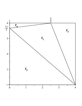
Figure 3. The square ${\mathfrak{q}}$ subdivided into 4 triangles $T_{i}$. Lattice subspaces parallel to the subspace $L={\mathbb{R}}(0,1)$ intersect the walls between the triangles at most in a point, and thus $S^{L}$ vanishes on the intersections of the triangles.

Table 1. Intermediate valuations of the square and the 4 triangles

${\mathfrak{p}}$	Vertices ${\mathcal{V}}({\mathfrak{p}})$	Intermediate valuation $S^{L}({\mathfrak{p}})$
$T_{1}$	$\left(\!\begin{smallmatrix}4\\ 0\end{smallmatrix}\!\right),\left(\!\begin{smallmatrix}\frac{5}{2}\\ 4\end{smallmatrix}\!\right),\left(\!\begin{smallmatrix}0\\ \frac{11}{3}\end{smallmatrix}\!\right)$	${\frac{{{\mathrm{e}}^{4\,x}}}{\left(1-{{\mathrm{e}}^{-x+\frac{8}{3}y}}\right)y}}-\frac{{\mathrm{e}}^{4\,x}}{\left(1-{{\mathrm{e}}^{-x+{\frac{11}{12}}\,y}}\right){y}}+{\frac{{{\mathrm{e}}^{3\,x+\frac{8}{3}y}}}{\left(1-{{\mathrm{e}}^{x-\frac{8}{3}\,y}}\right)y}}$
		${}-\frac{{\mathrm{e}}^{3\,x+{\frac{61}{15}}\,y}}{\left(1-{{\mathrm{e}}^{x+\frac{2}{15}y}}\right){y}}-\frac{{\mathrm{e}}^{\frac{11}{3}\,y}}{\left(1-{{\mathrm{e}}^{x-{\frac{11}{12}}\,y}}\right){y}}+{\frac{{{\mathrm{e}}^{\frac{11}{3}\,y}}}{\left(1-{{\mathrm{e}}^{x+\frac{2}{15}y}}\right)y}}$
$T_{2}$	$\left(\!\begin{smallmatrix}0\\ 0\end{smallmatrix}\!\right),\left(\!\begin{smallmatrix}4\\ 0\end{smallmatrix}\!\right),\left(\!\begin{smallmatrix}0\\ \frac{11}{3}\end{smallmatrix}\!\right)$	$-{\frac{1}{\left(1-{{\mathrm{e}}^{x}}\right)y}}-{\frac{{{\mathrm{e}}^{4\,x}}}{\left(1-{{\mathrm{e}}^{-x}}\right)y}}+\frac{{\mathrm{e}}^{4\,x}}{\left(1-{{\mathrm{e}}^{-x+{\frac{11}{12}}\,y}}\right){y}}+\frac{{\mathrm{e}}^{\frac{11}{3}\,y}}{\left(1-{{\mathrm{e}}^{x-{\frac{11}{12}}\,y}}\right){y}}$
$T_{3}$	$\left(\!\begin{smallmatrix}\frac{5}{2}\\ 4\end{smallmatrix}\!\right),\left(\!\begin{smallmatrix}4\\ 0\end{smallmatrix}\!\right),\left(\!\begin{smallmatrix}4\\ 4\end{smallmatrix}\!\right)$	$-{\frac{{{\mathrm{e}}^{3\,x+\frac{8}{3}y}}}{\left(1-{{\mathrm{e}}^{x-\frac{8}{3}y}}\right)y}}+{\frac{{{\mathrm{e}}^{3\,x+4\,y}}}{\left(1-{{\mathrm{e}}^{x}}\right)y}}-{\frac{{{\mathrm{e}}^{4\,x}}}{\left(1-{{\mathrm{e}}^{-x+\frac{8}{3}y}}\right)y}}+{\frac{{{\mathrm{e}}^{4\,x+4\,y}}}{\left(1-{{\mathrm{e}}^{-x}}\right)y}}$
$T_{4}$	$\left(\!\begin{smallmatrix}\frac{5}{2}\\ 4\end{smallmatrix}\!\right),\left(\!\begin{smallmatrix}0\\ 4\end{smallmatrix}\!\right),\left(\!\begin{smallmatrix}0\\ \frac{11}{3}\end{smallmatrix}\!\right)$	${\frac{{{\mathrm{e}}^{2\,x+4\,y}}}{\left(1-{{\mathrm{e}}^{-x}}\right)y}}-\frac{{\mathrm{e}}^{2\,x+{\frac{59}{15}}\,y}}{\left(1-{{\mathrm{e}}^{-x-\frac{2}{15}y}}\right){y}}+{\frac{{{\mathrm{e}}^{4\,y}}}{\left(1-{{\mathrm{e}}^{x}}\right)y}}-{\frac{{{\mathrm{e}}^{\frac{11}{3}\,y}}}{\left(1-{{\mathrm{e}}^{x+2/15\,y}}\right)y}}$
${\mathfrak{q}}$	$\left(\!\begin{smallmatrix}0\\ 0\end{smallmatrix}\!\right),\left(\!\begin{smallmatrix}0\\ 4\end{smallmatrix}\!\right),\left(\!\begin{smallmatrix}4\\ 4\end{smallmatrix}\!\right),\left(\!\begin{smallmatrix}4\\ 0\end{smallmatrix}\!\right)$	$\tfrac{{\mathrm{e}}^{4y}-1}{y}(1+{\mathrm{e}}^{x}+{\mathrm{e}}^{2x}+{\mathrm{e}}^{3x}+{\mathrm{e}}^{4x})$

Let $L={\mathbb{R}}(0,1)$. Let us apply the inclusion-exclusion formula together with the valuation property of $S^{L}$. As $S^{L}$ vanishes on the edges and vertices which occur in the intersections of the triangles, it follows that the sum $\sum_{i=1}^{4}S^{L}(T_{i})$ must be equal to $S^{L}({\mathfrak{q}})$.

The example has been chosen so that the intermediate valuation $S^{L}({\mathfrak{q}})$ can also be computed directly by elementary means. This allows us to verify our methods on the example. A direct computation gives

$$S^{L}({\mathfrak{q}})=\tfrac{{\mathrm{e}}^{4y}-1}{y}(1+{\mathrm{e}}^{x}+{\mathrm{e}}^{2x}+{\mathrm{e}}^{3x}+{\mathrm{e}}^{4x}).$$

Table 1 shows the output of our Maple program that implements the algorithm of the theorem for $S^{L}(T_{i})$, $i=1,\dots,4$. The equality $\sum_{i=1}^{4}S^{L}(T_{i})=S^{L}({\mathfrak{q}})$ is readily checked on these expressions.

4. Ehrhart quasipolynomials for intermediate valuations

Let us fix a rational polytope ${\mathfrak{p}}$ and a weight $h(x)$. It is well known (“Ehrhart’s Theorem”) that when we dilate ${\mathfrak{p}}$ by an integer $t\in{\mathbb{N}}$, the function $t\mapsto S(t{\mathfrak{p}},h)$ is a quasi-polynomial function of $t$ of degree $d+M$ where $M$ is the degree of $h$,

$$S(t{\mathfrak{p}},h)=\sum_{m=0}^{d+M}E_{m}({\mathfrak{p}},h;t)\,t^{m}.$$ (13)

The coefficients $E_{m}({\mathfrak{p}},h;t)$ depend only on $\{t\}_{q}$ where $q$ is an integer such that $q{\mathfrak{p}}$ has lattice vertices. When ${\mathfrak{p}}$ is a lattice polytope, then the coefficients $E_{m}({\mathfrak{p}},h;t)$ do not depend on $t$, and $t\mapsto S(t{\mathfrak{p}},h)$ becomes a polynomial.

E. Linke [13] has proved that the expression (13) is still valid for real dilations $t\in{\mathbb{R}}$. This is the generalized setting that we are going to use in this section. Note that if we allow real dilations, then even for lattice polytopes ${\mathfrak{p}}$ we obtain a quasi-polynomial rather than a polynomial; the fractional part function $\{\cdot\}_{q}$ with $q=1$ appears in the expressions for the coefficients $E_{m}({\mathfrak{p}},h;t)$. For instance, the number of integers in the interval $[0,t]=t[0,1]$ is $t+1-\{t\}_{1}$.

We are going to extend Ehrhart’s Theorem to the intermediate valuation $S^{L}({\mathfrak{p}})$. Indeed, one still has

$$S^{L}(t{\mathfrak{p}},h)=\sum_{m=0}^{d+M}E_{m}^{L}({\mathfrak{p}},h;t)\,t^{m}$$ (14)

where the coefficients $E^{L}_{m}({\mathfrak{p}},h;t)$ depend only on $\{t\}_{q}$. Note that when $L=V$, then $S^{L}(t{\mathfrak{p}},h)$ is polynomial, and coincides with the integral of $h$ on $t{\mathfrak{p}}$.

More precisely, we will show that the Ehrhart coefficients are step-polynomial functions of $t$, in the sense of [14]. In the next theorem, we prove these results and furthermore, we show that the coefficients $E_{m}^{L}({\mathfrak{p}},h;t)$ are given by short formulas, provided that in the input $(L,{\mathfrak{p}},h)$, the subspace $L$ has fixed codimension, ${\mathfrak{p}}$ is a simple polytope given by its vertices, and the weight is a power of a linear form $h(x)=\langle\ell,x\rangle^{M}$.

Theorem 28.

For every fixed number  $k_{0}\in{\mathbb{N}}$, there exists a polynomial-time algorithm for the following problem.

Input:

1. a number $d\in{\mathbb{N}}$ in unary encoding, with $d\geq k$,

2. a rational subspace $L\subseteq{\mathbb{R}}^{d}$ of codimension ${k_{0}}$, represented by $d-{k_{0}}$ linearly independent vectors $b_{1},\ldots,b_{d-{k_{0}}}\in{\mathbb{Q}}^{d}$ in binary encoding,

3. a finite index set ${\mathcal{V}}$,

4. a simple rational polytope ${\mathfrak{p}}$, given by the set ${\mathcal{V}}$ of its vertices, rational vectors $s_{i}\in{\mathbb{Q}}^{d}$ in binary encoding,

5. a rational vector $\ell\in{\mathbb{Q}}^{d}$ in binary encoding,

6. a number $M\in{\mathbb{N}}$ in unary encoding.

Output:

1. a finite index set $\Gamma$,

2. polynomials $f^{\gamma,m}\in{\mathbb{Q}}[r_{1},\ldots,r_{k_{0}}]$ and numbers $\zeta_{i}^{\gamma,m}\in{\mathbb{Z}}$, $q_{i}^{\gamma,m}\in{\mathbb{N}}$ for $\gamma\in\Gamma$, $i=1,\dots,k_{0}$ and $m=1,\dots,d+M$,

such that for $t\in{\mathbb{R}}$ we have $S^{L}(t{\mathfrak{p}},\langle\ell,x\rangle^{M})=\sum_{m=0}^{d+M}E_{m}(t)\,t^{m}$, where $E_{m}(t)$ is given by the step-polynomial

$$E_{m}(t)=\sum_{\gamma\in\Gamma}f^{\gamma,m}\bigl{(}\{\zeta_{1}^{\gamma,m}t\}_{q_{1}^{\gamma,m}},\dots,\{\zeta_{k_{0}}^{\gamma,m}t\}_{q_{k_{0}}^{\gamma,m}}\bigr{)}.$$

Remark 29.

Similar results hold for a more general weight $h(x)$, as in [3] for integrals over a simplex. One can assume that the weight is given as a polynomial in a fixed number $D$ of linear forms, $h(x)=f(\langle\ell_{1},x\rangle,\dots,\langle\ell_{D},x\rangle)$, or has a fixed degree $D$.

Proof of Theorem 28.

As first observed in [4], the path from generating functions to Ehrhart quasi-polynomials relies on the following important property of functions $\phi(\xi)\in{\mathcal{M}}_{\ell}(V^{*})$: such a function has a unique expansion into homogeneous rational functions

$$\phi(\xi)=\sum_{m\geq m_{0}}\phi_{[m]}(\xi).$$

If $P$ is a homogeneous polynomial on $V^{*}$ of degree $p$, and $D$ a product of $r$ linear forms, then $\frac{P}{D}$ is an element in ${\mathcal{M}}_{\ell}(V^{*})$ homogeneous of degree $m=p-r$. For instance, $\frac{\xi_{1}}{\xi_{2}}$ is homogeneous of degree $0$. On this example, we observe that a function in ${\mathcal{M}}_{\ell}(V^{*})$ which has no negative degree terms need not be analytic.

For a fixed $t\in{\mathbb{R}}$, the polynomial function $\xi\mapsto S^{L}(t{\mathfrak{p}},\frac{\langle\xi,x\rangle^{M}}{M!})$ is the term of degree $M$ of of the holomorphic function $S^{L}(t{\mathfrak{p}})(\xi)$. Let ${\mathfrak{c}}_{s}$ be the supporting cone of ${\mathfrak{p}}$ at the vertex $s$. By Brion’s theorem applied to the semi-rational polytope $t{\mathfrak{p}}$, we write $S^{L}(t{\mathfrak{p}})(\xi)$ as the sum of the intermediate generating functions of the cones at the vertices $ts$, $s\in{\mathcal{V}}$, of the dilated polytope $t{\mathfrak{p}}$. The crucial point is that the cone ${\mathfrak{c}}_{s}$ does not change when the polytope is dilated.

$$S^{L}(t{\mathfrak{p}})(\xi)=\sum_{s\in{\mathcal{V}}}S^{L}(ts+{\mathfrak{c}}_{s})(\xi).$$ (15)

Let $q_{s}$ be the smallest integer such that $q_{s}s$ is a lattice point. Then $(t-\{t\}_{q_{s}})s$ is a lattice point, therefore we have

$$S^{L}(ts+{\mathfrak{c}}_{s})(\xi) = {\mathrm{e}}^{\langle\xi,(t-\{t\}_{q_{s}})s\rangle}S^{L}(\{t\}_{q_{s}}s+{\mathfrak{c}}_{s})(\xi)$$

$$= {\mathrm{e}}^{t\langle\xi,s\rangle}{\mathrm{e}}^{-\langle\xi,\{t\}_{q_{s}}s\rangle}S^{L}(\{t\}_{q_{s}}s+{\mathfrak{c}}_{s})(\xi).$$

Expanding ${\mathrm{e}}^{t\langle\xi,s\rangle}$ in powers of $t$ and looking for the coefficient of $t^{i}$, we obtain

$$S^{L}\bigl{(}t{\mathfrak{p}},\tfrac{\langle\xi,x\rangle^{M}}{M!}\bigr{)}=\sum_{i\geq 0}t^{i}\sum_{s\in{\mathcal{V}}}\tfrac{\langle\xi,s\rangle^{i}}{i!}\bigl{(}{\mathrm{e}}^{-\langle\xi,\{t\}_{q_{s}}s\rangle}S^{L}(\{t\}_{q_{s}}s+{\mathfrak{c}}_{s})(\xi)\bigr{)}_{[M-i]}.$$

Thus we must analyze the term of $\xi$-degree $M-i$ of

$${\mathrm{e}}^{-\langle\xi,\{t\}_{q_{s}}s\rangle}S^{L}(\{t\}_{q_{s}}s+{\mathfrak{c}}_{s})(\xi).$$

We use Formula (10) and consider the summands indexed by $\gamma\in\Gamma$, one at a time. From then on, the proof is entirely similar to the proof of Theorem 37 in [2], and we omit it. ∎

Example 30 (Example 27, continued).

Table 2 shows the output of our Maple program for the Ehrhart quasi-polynomials of the four triangles of Example 27 with respect to the weight $h=1$. Note that the dilating parameter $t$ is real.

Table 2. Intermediate Ehrhart quasi-polynomials of the square and the 4 triangles

${\mathfrak{p}}$	Ehrhart quasi-polynomial $S^{L}(t{\mathfrak{p}},1)$
$T_{1}$	${\frac{21}{4}}\,\mbox{\boldmath${t}^{2}$}-{\frac{7}{8}}\,\left(\{4\,t\}_{1}\right)^{2}-{\frac{7}{10}}\,\{-5\,t\}_{2}+{\frac{7}{8}}\,\{4\,t\}_{1}+{\frac{7}{20}}\,\left(\{-5\,t\}_{2}\right)^{2}$
$T_{2}$	${\frac{22}{3}}\,\mbox{\boldmath${t}^{2}$}+{\frac{11}{6}}\,\mbox{\boldmath${t}$}-{\frac{11}{24}}\,\left(\{4\,t\}_{1}\right)^{2}+{\frac{11}{24}}\,\{4\,t\}_{1}$
$T_{3}$	$3\,\mbox{\boldmath${t}^{2}$}+\bigl{(}2-4\,\{4\,t\}_{1}\bigr{)}\,\mbox{\boldmath${t}$}-\frac{1}{3}\left(\{-5\,t\}_{2}\right)^{2}+\frac{2}{3}\{-5\,t\}_{2}+\frac{4}{3}\left(\{4\,t\}_{1}\right)^{2}-\frac{4}{3}\{4\,t\}_{1}$
$T_{4}$	${\frac{5}{12}}\,\mbox{\boldmath${t}^{2}$}+\frac{1}{6}\,\mbox{\boldmath${t}$}-{\frac{1}{60}}\,\left(\{5\,t\}_{2}\right)^{2}+\frac{1}{30}\,\{5\,t\}_{2}$
${\mathfrak{q}}$	$16\,\mbox{\boldmath${t}^{2}$}+\bigl{(}4-4\,\{4\,t\}_{1}\bigr{)}\,\mbox{\boldmath${t}$}$

We obtain

$$\sum_{i=1}^{4}S^{L}(tT_{i}) =16\,{t}^{2}+4\,t-4\,t\{4\,t\}_{1}-\tfrac{1}{30}\,\{-5\,t\}_{2}$$

$$\qquad+\tfrac{1}{30}\,\{5\,t\}_{2}+{\tfrac{1}{60}}\,\left(\{-5\,t\}_{2}\right)^{2}-{\tfrac{1}{60}}\,\left(\{5\,t\}_{2}\right)^{2}$$

$$=16\,{t}^{2}+4\,t-4\,t\{4\,t\}_{1},$$

using a relation between fractional parts, $\{x\}^{2}-\{-x\}^{2}=\{x\}-\{-x\}$, for the simplification. Indeed, a direct calculation gives the same answer.

Setting aside considerations of efficient computation, we can prove the following theorem.

Theorem 31 (Real Ehrhart Theorem).

Let ${\mathfrak{p}}\subseteq{\mathbb{R}}^{d}$ be a rational polytope, $h$ be a polynomial function of degree $M$, and $L\subseteq{\mathbb{R}}^{d}$ be a rational subspace of codimension ${k_{0}}$. Then $t\mapsto S^{L}(t{\mathfrak{p}},h)$ is a quasi-polynomial function of $t\in{\mathbb{R}}_{>0}$. More precisely,

$$S^{L}(t{\mathfrak{p}},h)=\sum_{m=0}^{d+M}E_{m}^{L}({\mathfrak{p}},h;t)\,t^{m},$$ (16)

where $E_{m}^{L}({\mathfrak{p}},h;t)$ is a step-polynomial of the form

$$E_{m}(t)=\sum_{\gamma\in\Gamma}f^{\gamma,m}\bigl{(}\{\zeta_{1}^{\gamma,m}t\}_{q_{1}^{\gamma,m}},\dots,\{\zeta_{k_{0}}^{\gamma,m}t\}_{q_{k_{0}}^{\gamma,m}}\bigr{)}\quad\text{for $t\in{\mathbb{R}}_{>0}$,}$$

where $\Gamma$ is a finite index set, with polynomials $f^{\gamma,m}\in{\mathbb{Q}}[r_{1},\ldots,r_{k_{0}}]$ and numbers $\zeta_{i}^{\gamma,m}\in{\mathbb{Z}}$, $q_{i}^{\gamma,m}\in{\mathbb{N}}$ for $\gamma\in\Gamma$, $i=1,\dots,k_{0}$ and $m=1,\dots,d+M$.

Proof.

The polytope ${\mathfrak{p}}$ is no longer assumed to be simple, so we compute a triangulation of each of the vertex cones and use inclusion–exclusion to avoid overcounting. Using a decomposition of $h$ into powers of linear forms, then the method of the previous theorem gives the result. ∎

References

- [1] D. Avis and K. Fukuda, Reverse search for enumeration, Discrete Appl. Math. 65 (1996), no. 1–3, 21–46.
- [2] V. Baldoni, N. Berline, J. A. De Loera, M. Köppe, and M. Vergne, Computation of the highest coefficients of weighted Ehrhart quasi-polynomials of rational polyhedra, eprint arXiv:1011.1602 [math.CO], 2010.
- [3] by same author, How to integrate a polynomial over a simplex, Mathematics of Computation, posted online July 14, 2010.
- [4] V. Baldoni, N. Berline, and M. Vergne, Local Euler–Maclaurin expansion of Barvinok valuations and Ehrhart coefficients of rational polytopes, Contemporary Mathematics 452 (2008), 15–33.
- [5] A. I. Barvinok, Polynomial time algorithm for counting integral points in polyhedra when the dimension is fixed, Mathematics of Operations Research 19 (1994), 769–779.
- [6] by same author, Computing the Ehrhart quasi-polynomial of a rational simplex, Mathematics of Computation 75 (2006), 1449–1466.
- [7] A. I. Barvinok and J. E. Pommersheim, An algorithmic theory of lattice points in polyhedra, New Perspectives in Algebraic Combinatorics (L. J. Billera, A. Björner, C. Greene, R. E. Simion, and R. P. Stanley, eds.), Math. Sci. Res. Inst. Publ., vol. 38, Cambridge Univ. Press, Cambridge, 1999, pp. 91–147.
- [8] M. Brion, Points entiers dans les polyèdres convexes, Ann. Sci. École Norm. Sup. 21 (1988), no. 4, 653–663.
- [9] M. Brion and M. Vergne, Residue formulae, vector partition functions and lattice points in rational polytopes, J. Amer. Math. Soc. 10 (1997), 797–833.
- [10] J. A. De Loera, D. Haws, R. Hemmecke, P. Huggins, J. Tauzer, and R. Yoshida, LattE, version 1.2, Available from URL http://www.math.ucdavis.edu/~latte/, 2005.
- [11] M. Köppe, A primal Barvinok algorithm based on irrational decompositions, SIAM Journal on Discrete Mathematics 21 (2007), no. 1, 220–236.
- [12] M. Köppe and S. Verdoolaege, Computing parametric rational generating functions with a primal Barvinok algorithm, The Electronic Journal of Combinatorics 15 (2008), 1–19, #R16.
- [13] E. Linke, Rational Ehrhart quasi-polynomials, eprint arXiv:1006.5612 [math.CO], 2010.
- [14] S. Verdoolaege and K. M. Woods, Counting with rational generating functions, J. Symb. Comput. 43 (2008), no. 2, 75–91.