Tube width fluctuations of entangled stiff polymers

Abstract

The tube-like cages of stiff polymers in entangled solutions have been shown to exhibit characteristic spatial heterogeneities. We explain these observations by a systematic theory generalizing previous work by D. Morse (Phys. Rev. E 63:031502, 2001). With a local version of the binary collision approximation (BCA), the distribution of confinement strengths is calculated, and the magnitude and the distribution function of tube radius fluctuations are predicted. Our main result is a unique scaling function for the tube radius distribution, in good agreement with experimental and simulation data.

I Introduction

Entangled solutions of stiff polymers are minimal model systems to generate a fundamental understanding of the origin of the mechanical properties of the cytoskeleton. This complex polymer scaffold maintains the stability and integrity of animal cells and is comprised of three types of semiflexible filaments, microtubules, actin, and intermediate filaments, with backbone diameters in the nanometer range but persistence lengths on the order of $10^{-1}\dots 10^{3}\mu m$ Gittes et al. (1993); Isambert et al. (1995); Schopferer et al. (2009). Single stiff biopolymers exhibit a rich mechanical response Ghosh et al. (2007); Emanuel et al. (2007); Hallatschek et al. (2007); Obermayer and Frey (2009). In-vitro reconstituted solutions of such biopolymers hint at how cells can acquire a considerable macroscopic strength from a purely topological microscopic constraint and thermal fluctuations, utilizing a minimum amount of material. Though the individual polymers only have to respect a simple constraint, namely the mutual impenetrability of the polymer backbones, complex soft-solid mechanical behavior arises at densities that would correspond to a very dilute gas without polymerization and a certain flexibility allowing for thermal backbone undulations. To deform an entangled polymer, surrounding polymers need to be pushed out of the way, as familiar from knotted strings. This mechanism leads to confinement of the individual polymers in effective tube-like cages, from which they only escape very slowly by a snake-like motion called reptation Edwards (1967a); de Gennes (1971). The suppression of chain motion perpendicular to the tube backbone is responsible for the remarkable integrity of the transient network. A microscopic derivation of this confinement poses formidable theoretical challenges, and there has so far been little progress beyond the introduction of basic topological invariants characterizing polymer entanglement Edwards (1967b); Müller-Nedebock and Edwards (1999) and a phenomenological primitive path analysis Everaers et al. (2004).

Nevertheless, self-consistent approximations for the dynamics of rigid Sussman and Schweizer (2011a, b) and the equilibrium statistical mechanics of semiflexible Morse (2001) topologically entangled chains have been worked out, and these treatments can predict salient properties of the reptation dynamics and the postulated tube. For stiff but not rigid polymers, with a large but finite persistence length $l_{p}$, the tube confinement of the transverse fluctuations of a representative test chain is implemented by a harmonic potential of stiffness $\phi$. The confinement geometry is characterized by an entanglement (or collision) length $L_{e}\ll l_{p}$ and the tube width $R\ll L_{e}$ Odijk (1983); Semenov (1986), both of which are functions of $\phi$. The former is a measure of the average spacing between adjacent collisions with background polymers, each of which contribute an amount $k_{B}T$ to the average confinement energy of the test chain. The latter measures the magnitude of the confined thermal fluctuations (Fig. 1).

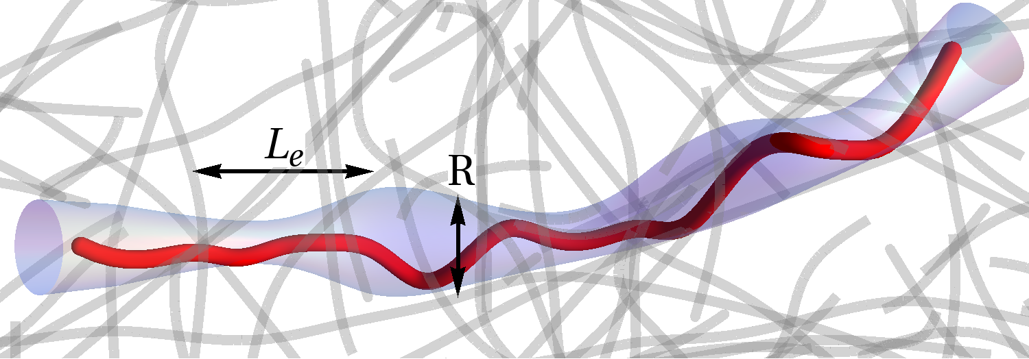
Figure 1: (Color online) Test polymer in a background solution, confined into a tube of spatially varying radius $R(s)$. The chemical distance $L_{e}$ indicates the characteristic scale of the tube heterogeneities.

Its mean value $\overline{R}$ as a function of monomer concentration has been predicted theoretically based on a binary collision approximation (BCA) and an effective medium approximation (EMA) Morse (2001). The BCA focuses on the pairwise entanglement topology of a test chain, while the EMA aims to account for the collective network fluctuations. More recently, these mean-field type theories have been challenged by the observation of pronounced heterogeneities of the local tube width $R(s)$ along the tube contour, which have been systematically studied in experiments Käs et al. (1994); Dichtl and Sackmann (1999); Romanowska et al. (2009); Wang et al. (2010); Glaser et al. (2010) and in simulations Hinsch et al. (2007). The tube heterogeneities have been statistically quantified by a broad and skewed tube width distribution $P(R)$, which has been analyzed by an empirical model Wang et al. (2010) and by a generalization of the BCA Glaser et al. (2010).

In the following, we develop a systematic, BCA-based theory to describe the fluctuations of the tube radius in an entangled polymer solution on the scale of individual tube collisions. Thereby, the local tube radius heterogeneities $R(s)$ and their distribution $P(R)$ can be determined, and $P(R)$ is found to be a universal non-Gaussian scaling function with a stretched tail. By comparison with the segment fluid approach of Ref. Glaser et al. (2010), in which the entangled solution is effectively mapped onto an ensemble of entanglement segments, we predict the segment length $L$ (which was previously treated as a fit parameter). The magnitude of the tube width fluctuations is compared with published experimental data. In Ref. Wang et al. (2010), $P(R)$ was instead estimated based on an ad-hoc distribution of the local mesh size. The result turned out to be unphysical at small values of $R$, however. As we show in the following, the fluctuations of the tube radius $R$ can be comprehensively described without additional assumptions based on a generalization of the BCA.

The remainder of the paper is organized as follows. In Sec. II, we introduce the fundamental concept of the tube and the wormlike chain (WLC) model for a single confined semiflexible polymer. In Sec. III, we then summarize the basic assumptions underlying the BCA as an approximation to the topological problem. Subsequently, in Sec. IV, we discuss the statistical distribution of the confinement strength, which explains the fluctuations of the tube radius, that are derived in Sec. V. In Sec. VI, the magnitude of tube radius fluctuations is used as an input to the segment fluid model, which predicts a scaling function for the tube radius distribution $P(R)$. The analytical results are compared to experimental data in Sec. VII.

II Basic elements of the tube model

II.1 Time scale separation and topology

We consider a stiff test polymer in the presence of surrounding uncrossable polymers, which are imposing topological constraints on its conformation. We restrict our discussion to tightly entangled polymers that are characterized by small transverse excursions around an average path, the preferred contour. The tube concept concerns quantities in an intermediate equilibrium, i.e. on time scales $\tau_{e}\ll t\ll\tau_{d}$, where $\tau_{e}$ is the time for the confined degrees of freedom to equilibrate inside the tube and $\tau_{d}$ is the disengagement time of the polymer from its initial tube. In what follows, a strong scale separation $\tau_{e}\ll\tau_{d}$ is assumed. Then, in the idealized limit $\tau_{d}\to\infty$, the topological relationships of the solution will be asymptotically conserved, and the average positions of the background polymers and their mutual topological relationships can be considered as effectively frozen (or “quenched”), thus collectively giving rise to a (quasi-static) confinement potential representing the tube. We denote the thermal average with respect to a given “quenched” configuration by angular brackets $\langle\cdots\rangle$ and the average over different configurations and topologies of the tube by an over-bar $\overline{\cdots}$. These ensemble averages correspond to temporal averages over several time intervals of length $\tau_{e}$ and $\tau_{d}$, respectively.

II.2 Statistical mechanics of a single entangled stiff polymer

II.2.1 Transverse distance distribution

To describe the physical properties of the test polymer, we assume that the effect of confinement can, to leading order, be described by a harmonic confinement potential. Hence, we use the weakly-bending Hamiltonian

$$H_{\mathrm{conf}}=\frac{l_{p}}{2}\int ds\,\left[\frac{\mathrm{d}^{2}\mathbf{r}_{\perp}(s)}{\mathrm{d}s^{2}}\right]^{2}+\frac{1}{2}\int ds\,\phi(s)\mathbf{r}_{\perp}^{2}(s)$$ (1)

for the transverse fluctuations $\mathbf{r}_{\perp}(s)$ of the test polymer about the straight ground state of a rigid rod, with a local confinement strength $\phi(s)$ that will be determined self-consistently. We use natural energy units ($k_{B}T=1$), such that the persistence length $l_{p}=\kappa/k_{B}T$ is synonymous with the bending rigidity $\kappa$. We define the arc-length dependent tube radius $R(s)$ via the variance of one component of the confined transverse fluctuations,

$$R^{2}(s)\equiv\frac{1}{2}\langle\mathbf{r}_{\perp}^{2}(s)\rangle.$$ (2)

Approximating the free energy by an effective Hamiltonian $H_{\mathrm{conf}}$ that is quadratic in the fluctuations $\mathbf{r}_{\perp}(s)$ is equivalent to approximating the distribution of $P[\mathbf{r}_{\perp}(s)]$ in a given configuration by a Gaussian. Experiments Dichtl and Sackmann (1999); Glaser et al. (2010); Wang et al. (2010) and simulations Zhou and Larson (2006); Hinsch et al. (2007) indicate that the distribution of transverse distances is indeed Gaussian for small transverse displacements $\mathbf{r}_{\perp}(s)$ on the order of the tube radius $R$. It can be shown theoretically, that this assumption is in accord with a self-consistent treatment of the tube Morse (2001).

II.2.2 Tube radius $R$ and entanglement length $L_{e}$

As a first step, we consider the case of a test polymer in a homogeneous (cylindrical) tube that can be characterized by the spatial average $\overline{\phi}$ of a local confinement strength $\phi(s)$, and hence a tube radius $R(s)\equiv R_{0}=const\,$. The variance of $\mathbf{r}_{\perp}(s)$ [Eq. (2)] is obtained from the tube Hamiltonian Eq. (1) via equipartition, such that

$$R^{2}(s) = \int\frac{\mathrm{d}q}{2\pi}\frac{1}{l_{p}q^{4}+\overline{\phi}}$$ (3)

$$= \frac{1}{2\sqrt{2}l_{p}^{1/4}\overline{\phi}^{3/4}}\equiv R_{0}^{2}$$ (4)

is the square of the tube radius corresponding to a homogeneous confinement strength $\overline{\phi}$. Heterogeneities of the tube potential and of the tube radius are discussed below (in Sections IV & V), where we show how small spatial fluctuations $\delta\phi(s)\equiv\phi(s)-\overline{\phi}$ lead to spatial variations of $R(s)$ about its average value $\overline{R}$. We assume in what follows that the peak of the corresponding distribution $P(R)$ is sufficently well defined such that the average $\overline{R}$ and the typical value $R_{0}$ can be used interchangeably.

The second characteristic quantity of the tube geometry, the entanglement length $L_{e}$, is defined by assigning a harmonic confinement energy equal to $k_{B}T$ ($=1$ in our units) to every collision, and identifying $L_{e}$ with the collision length. Writing $\overline{\phi}$ for the average confinement potential strength in Eq. (1), equipartition yields

$$L_{e}=\left[\int dq\frac{\overline{\phi}}{l_{p}q^{4}+\overline{\phi}}\right]^{-1}=2\sqrt{2}\frac{l_{p}^{1/4}}{\overline{\phi}^{1/4}}.$$ (5)

III BCA

We recapitulate the essential arguments that are needed to derive the BCA and to understand the reasoning that follows.

The BCA was designed as an approximation to the underlying topological many-body problem, suitable for estimating the absolute value of the average tube radius $\overline{R}$, self-consistently. One considers an elementary encounter (‘binary collision’) between two tubes, calculates the free energy of confinement due to the uncrossability of the chains, and sums over possible configurations of the pair of tubes. The key approximation consists in neglecting correlations between multiple collisions.

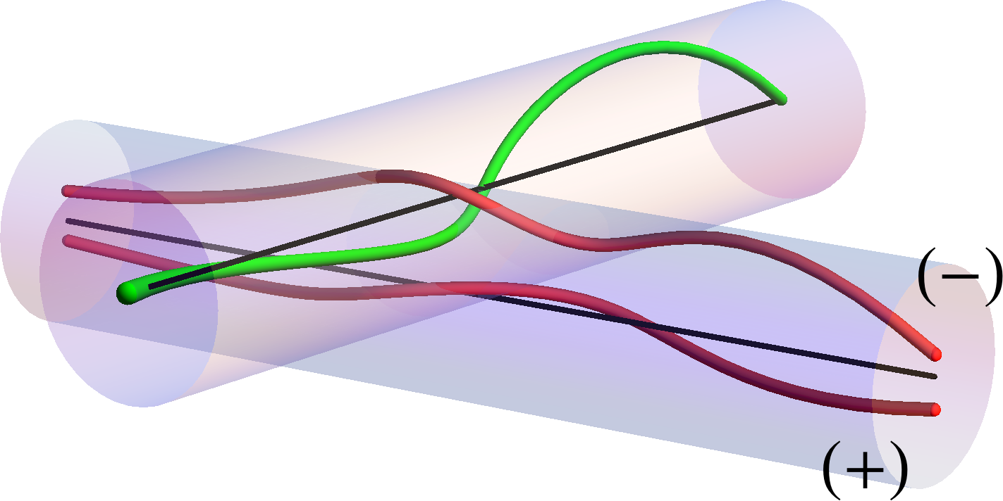
Figure 2: (Color online) Topology of two confined polymers inside their tubes at a collision point: for fixed preferred tube contours in the transparent state, the polymers are found either in the ‘above’ ($+$) or ‘below’ ($-$) configuration. Adapted from Ref. Morse (2001).

The dynamic entanglement problem is cast into equilibrium statistical mechanics language by assuming that the tube contours are (temporarily) frozen. In such a configuration, an arbitrarily chosen point on the tube contour associated with the test chain is characterized by a Gaussian distribution of transverse distances, as outlined in the preceding section. Its standard deviation is approximated by the average tube radius $\overline{R}$. Consider now a second background chain passing within a distance $\overline{R}$ from the chosen point on the test chain. We refer to this event as a tube collision. To calculate the contribution of the pair collision to the confinement free energy, the BCA distinguishes between two states: a hypothetical state, in which the test chain is transparent with respect to collisions with the background chain and a state in which the chains are mutually uncrossable. Due to the key assumption that the collisions along the test chain are uncorrelated, the environment of the collision point is completely random in the transparent state, i.e. the distribution of transverse distances is unchanged from the Gaussian distribution with standard deviation $\overline{R}$. The average free energy of confinement follows from a topological argument. In the uncrossable state for this pair of chains, the configuration space of transverse fluctuations is divided into two disconnected subspaces corresponding to the ‘above’ ($+$) and the ‘below’ ($-$) configuration, as depicted in Fig. 2. The average free energy in the uncrossable state is therefore obtained by averaging the confinement potential in each of these subspaces over the probability for a specific topology and collision geometry. The resulting average free energy is equated with that of the transparent state to obtain a self-consistent estimate of the tube radius $\overline{R}$.

For the original mathematical implementation of the above ideas we refer the reader to Ref. Morse (2001). We note that a slightly corrected estimate for the prefactor in the scaling result for the average tube radius $\overline{R}$ with concentration was calculated in Ref. Glaser et al. (2010) (supplement).

IV Distribution $P[\phi]$ of tube strengths

The original BCA is exclusively concerned with average values $\overline{R}$, $\overline{\phi}$. The scaling of these values with concentration $\rho$ has been tested experimentally Tassieri et al. (2008); Romanowska et al. (2009); Wang et al. (2010), but the prefactor is sensitive to the precise control of the experimental conditions and is usually treated as a fit factor. For a more detailed comparison of theory, experiment and simulations, knowledge not only of the average value but of the richer and more robust tube radius distribution $P(R)$ is desirable (cf. Sec. V).

As a first step towards calculating $P(R)$, we derive the distribution $P[\phi]$ of the local confinement strength $\phi(s)$ of a test polymer. Morse Morse (2001) gave an explicit expression for the confinement free energy of a test chain colliding with a medium chain. We will explicitly adopt the mathematical approximation of straight tube contours, that was implicitly made in the previous work, and it is shown that inconsistencies resulting from this approximation are avoided by verifying that the calculated quantities do not depend on the overall chain length. Let the distance of shortest approach between two preferred contours with orientations $\mathbf{u}$, $\mathbf{u}^{\prime}$ and centers of mass $\mathbf{r}$, $\mathbf{r}^{\prime}$ be $x=(\mathbf{r}-\mathbf{r}^{\prime})\cdot\mathbf{e}_{x}$, where $\mathbf{e}_{x}=\mathbf{u}\times\mathbf{u}^{\prime}/|\mathbf{u}\times\mathbf{u}^{\prime}|$ is the direction perpendicular to both preferred contours, then the free energy of the test polymer whose preferred contour has been uniformly displaced by a vector $\mathbf{h}=h\mathbf{e}_{h}$ is

$$F_{\pm}(\mathbf{h})=-\ln\Phi\left(\pm\frac{x-h\cos\psi}{\overline{R}}\right).$$ (6)

Here, the sign $\pm$ refers to the specific topology (cf. Fig. 2) and $\cos\psi=\mathbf{e}_{h}\cdot\mathbf{e}_{x}$. The function $\Phi(x)$ is given by the restricted partition sum of the Gaussian fluctuations of the test polymer in the presence of an uncrossable test chain Morse (2001),

$$\Phi(y)=\frac{1}{2}\mbox{erfc}\left(-\frac{y}{2}\right).$$ (7)

It can be interpreted as the probability $p_{\pm}(x)=\Phi(\pm x/\overline{R})$ of finding a specific topology.

From Eq. (6), we obtain the confinement strength $\phi$ in a given configuration of preferred contours and topology as the second derivative of the free energy,

$$\phi_{\pm}(x)=\frac{\mathrm{d^{2}}}{\mathrm{d}h^{2}}F_{\pm}(\mathbf{h})\Big{|}_{h=0}=-\frac{\cos^{2}\psi}{\overline{R}^{2}}\frac{\mathrm{d}^{2}}{\mathrm{d}y^{2}}\ln\Phi(y)\Big{|}_{\pm x/{\overline{R}}}.$$ (8)

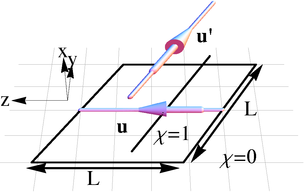
Figure 3: (Color online) Overlap area (parallelogram) of two tubes of length $L$, represented by their preferred contours with orientations $\mathbf{u}$, $\mathbf{u}^{\prime}$ enclosing an arbitrary angle, and characteristic function $\chi$.

To derive the distribution of confinement strengths $\phi(s)$, we now turn back to the central BCA approximation that the collisions between the test polymer and the background polymers are independent localized events. Due to the requirement $\overline{R}\ll L_{e}$, we may, without loss of generality, even treat them as point-like and express the confinement potential $\phi(s)$ per unit length at a point $s$ on the test polymer as

$$\phi(s)=\sum_{i=1}^{N}\chi(\mathbf{r}_{i},\mathbf{u}_{i},\mathbf{u})\delta(s-z_{i})\phi_{\pm}(x_{i}).$$ (9)

Here, $\chi(\mathbf{r}_{i},\mathbf{u}_{i},\mathbf{u})$ is a characteristic function of overlap between the colliding tubes, which takes on the value one whenever a tube collision occurs, and zero otherwise (for a graphical definition see Fig. 3). We introduce it, here, merely as a convenient tool to facilitate the formal manipulation of the following expressions. The coordinate $z_{i}$ in the argument of the $\delta$-function is the point of shortest approach (the collision point) between the two tubes on the test polymer.

The distribution $P[\phi]$ of confinement strengths that follows from Eq. (9) is of the Holtsmark type Holtsmark (1919); Simon et al. (1990) and describes the total confinement potential of the test chain as a sum of contributions resulting from uncorrelated collisions with medium chains. Explicitly, its moment-generating functional is given by (cf. App. A)

$$P[w(s)]=\exp\left[\frac{n}{2\pi}\sum_{\pm}\int\mathbf{d}\mathbf{r}^{\prime}\int^{\prime}\!d\mathbf{u}^{\prime}\,\chi e^{iw(z^{\prime})\phi_{\pm}(x^{\prime})}p_{\pm}(x^{\prime})\right].$$ (10)

From this, we obtain the average of $\phi(s)$ by functional differentiation of the logarithm of Eq. (10) with respect to the field $w(s)$ (cf. App. A),

$$\overline{\phi}=\frac{nL\pi}{8\overline{R}}\int d\tilde{x}\,\frac{\Phi^{\prime 2}(\tilde{x})}{\Phi(\tilde{x})}.$$ (11)

The integral in Eq. (11) is numerically evaluated and gives $\overline{\phi}=\alpha\,nL/\overline{R}$, with $\alpha=0.502$, in agreement with earlier results Morse (2001) (applying the slight numerical correction discussed in Ref. Glaser et al. (2010), supplement).

We proceed analogously to obtain the second cumulant (cf. App. A), the correlation function

$$\overline{\phi(s)\phi(s^{\prime})}=\beta\frac{nL}{\overline{R}^{3}}\delta(s-s^{\prime}),$$ (12)

where $\beta=0.0941$. The uncorrelated character of the collisions is apparent from the $\delta$-function on the RHS of Eq. (12). Both should be understood in the coarse-grained sense, assuming $\overline{\phi(s)\phi(s^{\prime})}=0$ when $s-s^{\prime}\gg\overline{R}$.

V Gaussian approximation to the tube radius distribution $P(R)$

We can now turn the distribution $P[\phi]$, which we characterized by its first two cumulants, into a Gaussian approximation to the tube radius distribution $P(R)$, by calculating the linear response of the local tube radius $R(s)$ to spatial changes (heterogeneities) in $\phi(s)$. We begin with the observation that the correlation function of the (projected) transverse fluctuations, $C(s,s^{\prime})=\langle\mathbf{r}_{\perp}(s)\cdot\mathbf{r}_{\perp}(s^{\prime})\rangle/2$ obeys the following differential equation (cf. App. B)

$$-l_{p}\partial_{s}^{4}C(s,s^{\prime})-\phi(s^{\prime})C(s,s^{\prime})=\delta(s-s^{\prime})$$ (13)

The tube radius is given by $R(s)=[C(s,s)]^{1/2}$ and the linear response expression for this quantity is calculated in App. B as

$$R(s)=\overline{R}-\frac{1}{2\overline{R}}\int ds^{\prime}\,G^{2}(s-s^{\prime})\delta\phi(s^{\prime}).$$ (14)

The variance of the tube radius $R(s)$ at a randomly chosen point $s$ on the test polymer is now calculated from Eq. (14) as

$$\overline{\delta R^{2}}\equiv\overline{[R(s)-\overline{R}]^{2}}$$ (15)

$$=\frac{1}{4\overline{R}^{2}}\int ds^{\prime}ds^{\prime\prime}\,G^{2}(s-s^{\prime})G^{2}(s-s^{\prime\prime})\overline{\phi(s^{\prime})\phi(s^{\prime\prime})}.$$

Within the BCA, with its trivial spatial correlations of the confinement potential $\phi(s)$, Eq. (12), this reduces to

$$\overline{\delta R^{2}}=\beta\frac{nL}{4\overline{R}^{5}}\int ds^{\prime}G^{4}(s-s^{\prime}).$$ (16)

The integral Eq. (16) is numerically evaluated using an explicit expression for $G(s)$ [Eq. (34)],

$$\int ds\,G^{4}(s)=\gamma\,\overline{R}^{8}L_{e},$$ (17)

where $\gamma=0.5125$, which yields the final result for the variance of $P(R)$,

$$\overline{(\delta R)^{2}}=\frac{1}{4}\beta\gamma nL\overline{R}^{3}L_{e}.$$ (18)

Using the self-consistent solutions for $\overline{R}=(4\alpha)^{-3/5}(nL)^{-3/5}l_{p}^{-1/5}$ and $L_{e}=(\alpha/8)^{-2/5}(nL)^{-2/5}l_{p}^{1/5}$ Morse (2001), mean and variance of the Gaussian approximation to the tube radius distribution $P(R)$ are completely determined in terms of the contour length concentration $nL$ and the persistence length $l_{p}$. In particular, the coefficient of variation $c_{v}=[\overline{(\delta R)^{2}}]^{1/2}/\overline{R}$ turns out to be a concentration-independent constant,

$$c_{v}=\frac{1}{2}\sqrt{\frac{\beta\gamma}{\alpha}}=0.155.$$ (19)

VI Segment fluid approximation

In Ref. Glaser et al. (2010), a broad distribution $P(R)$ of the tube radius was found. The derivation of an analytical result for this distribution was also based on a Holtsmark-type distribution for the confinement strength $\phi$ resulting from uncorrelated collisions, but the latter were averaged over the characteristic length $L$ of entanglement segments (which is why the approach was called a “segment-fluid” approximation). It was argued that this length is on the order of $L_{e}$. We now show that this choice is indeed justified and predict the precise value of the segment length.

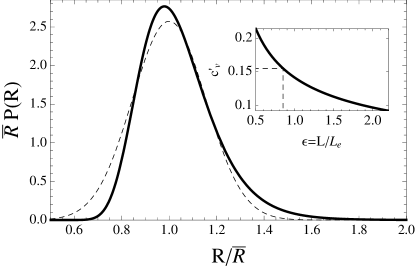
Figure 4: (Color online) Reduced distribution $\overline{R}P(R/\overline{R})$ of the tube radius $R$. The solid line is the segment-fluid prediction, the dashed line is a Gaussian approximation with coefficient of variation $c_{v}$ given by Eq. (19). Inset: Coefficient of variation $c^{\prime}_{v}$ of the segment fluid approximation versus reduced segment length $\epsilon=L/L_{e}$, and the predicted value.

The tube radius distribution $P(R)$ was given as an analytical approximation in Ref. Glaser et al. (2010),

$$P(R)=\frac{8}{3R\Gamma(k)}\exp(-y)\,y^{k},\quad y\equiv 0.01325\,\frac{L\overline{R}^{2}}{\ell_{p}^{1/3}R^{8/3}},$$ (20)

where $k=4.013n^{\prime}L^{2}\overline{R}$, $n^{\prime}$ is the number density of entanglement segments and $\Gamma(x)$ is the Gamma function. It was noted Glaser et al. (2010) that $P(R)$ can be written as a scaling function $P(R)=(1/\overline{R})f(R/\overline{R},n^{\prime}L^{2}\overline{R})$. This implies that the coefficient of variation is given by a constant, $c^{\prime}_{v}=g(n^{\prime}L^{2}\overline{R})$. If we make the ansatz $L=\epsilon L_{e}$, with an undetermined dimensionless constant $\epsilon$ and use the self-consistent values for $\overline{R}$ and $L_{e}$ given above, we get $c^{\prime}_{v}=g(\epsilon/\alpha)$. The function $g(x)$ is easily evaluated numerically and is shown in Fig. 4 (inset). To fix $\epsilon$ and thus the length $L$ of entanglement segments, we require $c^{\prime}_{v}=c_{v}$ and obtain numerically $\epsilon=0.85$.

Evaluating the tube radius distribution $P(R)$ [Eq. (20)] at this value of the reduced segment length $L/L_{e}$, we obtain $k=y(R/\overline{R})^{8/3}=6.79$ and hence all parameters occurring in $P(R)$ are now fully specified, giving

$$P(R)=N\exp\left[-6.79\left(\frac{\overline{R}}{R}\right)^{8/3}\right](\overline{R}/R)^{8/3},$$ (21)

with a normalization constant $N=2.434\times 10^{3}$. The corresponding unique reduced distribution $\overline{R}P(R)$ is shown in Fig. 4 and compared to the Gaussian distribution with the same $c_{v}$. Beyond what was achieved in Ref. Glaser et al. (2010), the functional form of $P(R)$ is now fully determined. As can be seen in Fig. 4, the distribution $P(R)$ is positively skewed and has a broad tail at large values of $R$.

VII Comparison to experiment

The functional form of $P(R)$ was compared to experimental data in Ref. Glaser et al. (2010), and very good qualitative agreement was found, using the value of the segment length $L$ as a fit parameter. Remarkably, also our above prediction of a constant value for the coefficient of variation $c_{v}$, which can be checked against a whole set of independent measurements, is nicely confirmed by the data (Fig. 5).

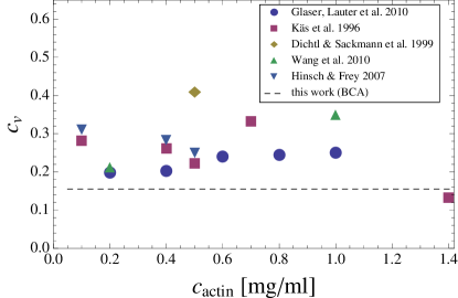
Figure 5: (Color online) Comparison of tube radius fluctuations in different experiments and simulations of semidilute solutions of F-actin. Shown is the coefficient of variation $c_{v}=\sqrt{\overline{\delta R^{2}}}/\overline{R}$ for the fluctuations of $R$. Symbols correspond to data taken from the literature. Circles: experimental data taken from Ref. Glaser et al. (2010) (Fig. 3, inset); squares: experimental data from Ref. Käs et al. (1996); diamonds: experimental data from Ref. Dichtl and Sackmann (1999) for the fluctuations of the response coefficient $\alpha_{\perp}$, converted to fluctuations of the tube radius $R$; upright triangles: experimental data from Wang et al. (2010) (Fig. 2); downward facing triangles: simulation data from Ref. Hinsch et al. (2007) (Fig. 9). The solid dashed line is the prediction of Eq. (19).

The figure summarizes literature data for $c_{v}$ against monomer concentration $c$ from various experiments and simulations of semidilute actin solutions. The dashed line is our prediction from Eq. (19). Two results are evident from this plot. First, the data scatter within a band of $c_{v}=0.2$-$0.4$. Second, the theoretical prediction lies below most of the data points and thus provides a lower bound for the observed tube radius fluctuations. This suggests that a constant value for the coefficient of variation is indeed consistent with the reported data, but that the heterogeneities are actually about twice as strong as predicted.

This is not entirely unexpected, since the BCA, on which our theoretical derivation relies, is not meant to describe the absolute value of the tube radius quantitatively. In fact, the BCA alone is well known to underestimate the tube fluctuations, since it does not take into account the collective fluctuations of the surrounding medium into which the tube is embedded Morse (2001). Corresponding quantitative discrepancies with experiments have been reported before Tassieri et al. (2008).

VIII Conclusion

We have calculated the fluctuations of the tube radius in entangled solutions of semiflexible polymers, based on the binary collision approximation (BCA). We predict that the shape of the tube radius distribution is given by a universal (concentration-independent) scaling function, for which we gave an analytical approximation in Eq. (21). Our results provide a quantitative characterization of the local packing structure of entangled biopolymer solutions in terms of distribution functions, which are at the same time a more sensitive and more robust means for comparing data and theory than average values alone. We hope that the methods of analysis established here may find application in future experimental studies, e.g. in microrheology Waigh (2005); Wirtz (2009), or in the interpretation of simulation data Hinsch et al. (2007); Ramanathan and Morse (2007). Further theoretical questions, such as the characterization of the distribution of tube contours Hinsch and Frey (2009); Romanowska et al. (2009), are currently under study.

Appendix A Calculation of the distribution of confinement strengths $P[\phi]$

The distribution of the local confinement strength is formally obtained as the average $P[\varphi(s)]=\overline{\delta[\phi(s)-\varphi(s)]}$ over all possible configurations of tube contours and topologies. The corresponding characteristic functional, $P[w(s)]$, follows from a functional Fourier transform and Eq. (9) as

$$P[w(s)]=\overline{\exp\left(i\sum_{i=1}^{N}\chi(\mathbf{r}_{i},\mathbf{u}_{i},\mathbf{u})w(z_{i})\phi_{\pm}(x_{i})\right)}.$$ (22)

Here, tangents to the test and the background chains’ tube backbones are denoted by $\mathbf{u}$ and $\mathbf{u}_{i}$, and the vector $\mathbf{r}_{i}$ connects the tubes’ center of mass of the test chain with that of the background chain $i$. Its coordinates $x_{i}$, $y_{i}$ and $z_{i}$ are defined along the directions $\mathbf{e}_{x,i}=(\mathbf{u}\times\mathbf{u}_{i})/|\mathbf{u}\times\mathbf{u}_{i}|$, $\mathbf{e}_{y,i}=\mathbf{u}\times\mathbf{e}_{x,i}$ and $\mathbf{e}_{z,i}=\mathbf{u}$. The quenched average $\overline{\cdots}$ is implemented as the simultaneous average over the probability $p_{\pm}(x_{i})=\Phi(\pm x_{i})$ of finding a specific topology ‘+’ or ’-’ [defined after Eq. (7)] and over the uniformly distributed centers of mass and orientations of the tubes. Since the chains’ preferred contours are assumed to be uncorrelated, the average over the $N$ preferred contours and the topology of the background chains relative to the test chain factorizes as

$$P[w(s)]=\left[\sum_{\pm}\int\frac{d\mathbf{r}^{\prime}}{V}\int^{\prime}\frac{d\mathbf{u}^{\prime}}{2\pi}e^{i\chi(\mathbf{r}^{\prime},\mathbf{u}^{\prime},\mathbf{u})w(z^{\prime})\phi_{\pm}(x^{\prime})}p_{\pm}(x^{\prime})\right]^{N}.$$ (23)

Here, the integral over orientations extends over the half-sphere (indicated by a prime). Exploiting the formal definition of $\chi$ as a characteristic function of overlap, which amounts to setting the factor in the brackets for non-overlapping chains to unity (since the probability $p_{\pm}(x^{\prime})$ is normalized), we get

$$P[w(s)]$$ (24)

$$=\left\{1+\sum_{\pm}\int\frac{d\mathbf{r}^{\prime}}{V}\int^{\prime}\frac{d\mathbf{u}^{\prime}}{2\pi}\left[e^{iw(z^{\prime})\phi_{\pm}(x^{\prime})}p_{\pm}(x^{\prime})-1\right]\chi\right\}^{N}.$$

Using $n=N/V$ for the polymer number concentration and performing the limit $N\to\infty$, Eq. (10) in the main text is obtained.

The first cumulant is obtained by functional differentiation of the characteristic functional Eq. (10) with respect to the field $w(s)$,

$$\overline{\phi(s)} =-i\frac{\delta}{\delta w(s)}\ln P[w(s)]\Big{|}_{w(s)=0}$$ (25)

$$=\frac{nL}{2\pi}\sum_{\pm}\int^{\prime}d\mathbf{u}^{\prime}\,\int d\mathbf{r}^{\prime}\,\delta(z^{\prime}-s)\chi p_{\pm}(x^{\prime})\phi_{\pm}(x^{\prime}).$$ (26)

Using the fact that the integral of $\chi\delta(z^{\prime}-s)$ over $dy^{\prime}$ and $dz^{\prime}$ is the height $L\sin\theta$ of the overlap area (Fig. 3), carrying out the second derivative of $-\ln\Phi$ and the angular integrals, and using $\sum_{\pm}\Phi(x^{\prime})=1$, one arrives at Eq. (11) in the main text. Analogously, we obtain the second cumulant, the correlation function

$$\overline{\phi(s)\phi(s^{\prime})}$$ (27)

$$=-\frac{\delta^{2}}{\delta w(s)\delta w(s^{\prime})}\ln P[w(s)]\Big{|}_{w(s)=0}$$ (28)

$$=\frac{nL}{2\pi}\sum_{\pm}\int^{\prime}d\mathbf{u}^{\prime}\,\int d\mathbf{r}^{\prime}\,\delta(z^{\prime}-s)\delta(z^{\prime}-s^{\prime})\chi p_{\pm}(x^{\prime})\phi_{\pm}^{2}(x^{\prime}).$$ (29)

Applying a similar reasoning as above to simplify the equation and numerically evaluating the remaining $x$-integral, we obtain Eq. (12) in the main text.

Appendix B Heterogeneous tube radius $R(s)$

The fluctuation-response relation Eq. (13) for the correlation function $C(s,s^{\prime})$ is derived from the free energy $-\ln Z[\mathbf{f}_{\perp}(s)]$ of a confined WLC in the presence of an external transverse force $\mathbf{f}_{\perp}(s)$. The corresponding Hamiltonian is $H=H_{\mathrm{conf}}+\int ds\,\mathbf{f}_{\perp}(s)\mathbf{r}_{\perp}(s)$. Since

$$\langle\mathbf{r}_{\perp}(s)\rangle =\frac{\delta\ln Z}{\delta\mathbf{f}_{\perp}(s)},$$ (30)

$$\langle\mathbf{r}_{\perp}(s)\mathbf{r}_{\perp}(s^{\prime})\rangle =\frac{\delta\ln Z}{\delta\mathbf{f}_{\perp}(s)\delta\mathbf{f}_{\perp}(s^{\prime})}\Big{|}_{\mathbf{f}_{\perp}(s)=0}$$ (31)

$$=\frac{\delta\langle\mathbf{r}_{\perp}(s)\rangle}{\delta\mathbf{f}_{\perp}(s^{\prime})}\Big{|}_{\mathbf{f}_{\perp}(s)=0},$$ (32)

it follows that $\mathbf{C}(s,s^{\prime})\equiv\langle\mathbf{r}_{\perp}(s)\mathbf{r}_{\perp}(s^{\prime})\rangle$ is the functional inverse of $\mathbf{C}(s,s^{\prime})^{-1}=\delta\mathbf{f}_{\perp}(s)/\delta{\langle}\mathbf{r}_{\perp}(s^{\prime}){\rangle}$. Since the force $\mathbf{f}_{\perp}(s)=-{\langle}\delta H_{\mathrm{conf}}/\delta\mathbf{r}_{\perp}(s){\rangle}$ producing an average displacement ${\langle}\mathbf{r}_{\perp}(s){\rangle}$ is given by $-l_{p}\partial_{s}^{4}\langle\mathbf{r}_{\perp}(s)\rangle-\phi(s)\langle\mathbf{r}_{\perp}(s)\rangle$, Eq. (13) follows by partial integration.

A solution of Eq. (13) would exactly describe the tube heterogeneities that follow from a heterogeneous confinement potential $\phi(s)$. However, no such solution is available for arbitrary $\phi(s)$. Therefore, we write $\phi(s)=\overline{\phi}+\delta\phi(s)$ with small fluctuations $\delta\phi(s)$ about the average confinement strength $\overline{\phi}$. A simple first-order perturbation scheme for $C(s,s^{\prime})=C^{(0)}(s,s^{\prime})+\delta C(s,s^{\prime})$ is set up by requiring $C^{(0)}$ to be the response function in the homogeneous case, where $\delta\phi(s)=0$,

$$C^{(0)}(s-s^{\prime})=G(s-s^{\prime})=\int\frac{dq}{2\pi}\frac{e^{iq(s-s^{\prime})}}{l_{p}q^{4}+\overline{\phi}}.$$ (33)

The explicit expression for the Fourier transform in Eq. (33) can be obtained analytically and written [using Eqs. (4) & (5)] as

$$G(s-s^{\prime})=R_{0}^{2}\,e^{-2|s|/L_{e}}\left[\cos\left(2\frac{s}{L_{e}}\right)+\sin\left(2\frac{|s|}{L_{e}}\right)\right].$$ (34)

The leading-order response $\delta C(s,s^{\prime})$ to the perturbation $\delta\phi(s,s^{\prime})$ is obtained from Eq. (13) if small terms $\mathcal{O}(\delta C\delta\phi)$ are neglected,

$$\delta C(s,s^{\prime})=-\int ds^{\prime\prime}G(s-s^{\prime\prime})\delta\phi(s^{\prime\prime})G(s^{\prime}-s^{\prime\prime}).$$ (35)

Eq. (14) in the main text is obtained by writing $R(s)=\overline{R}+\delta R(s)$ with $\delta R(s)=\delta(R^{2})/2\overline{R}=\delta C(s,s)/2R_{0}$.

References

- Gittes et al. (1993) F. Gittes, B. Mickey, J. Nettleton, and J. Howard, The Journal of cell biology 120, 923 (1993).
- Isambert et al. (1995) H. Isambert, P. Venier, A. Maggs, A. Fattoum, R. Kassab, D. Pantaloni, and M. Carlier, Journal of Biological Chemistry 270, 11437 (1995).
- Schopferer et al. (2009) M. Schopferer, H. Bär, B. Hochstein, S. Sharma, N. Mücke, H. Herrmann, and N. Willenbacher, Journal of molecular biology 388, 133 (2009).
- Ghosh et al. (2007) A. Ghosh, J. Samuel, and S. Sinha, Physical Review E 76, 061801 (2007).
- Emanuel et al. (2007) M. Emanuel, H. Mohrbach, M. Sayar, H. Schiessel, and I. M. Kulić, Physical Review E 76, 61907 (2007).
- Hallatschek et al. (2007) O. Hallatschek, E. Frey, and K. Kroy, Physical Review E 75, 031906 (2007).
- Obermayer and Frey (2009) B. Obermayer and E. Frey, Physical Review E 80, 040801(R) (2009).
- Edwards (1967a) S. F. Edwards, Proceedings of the Physical Society London 92, 9 (1967a).
- de Gennes (1971) P. G. de Gennes, The Journal of Chemical Physics 55, 572 (1971).
- Edwards (1967b) S. F. Edwards, Proceedings of the Physical Society 91, 513 (1967b).
- Müller-Nedebock and Edwards (1999) K. K. Müller-Nedebock and S. F. Edwards, J. Phys. A: Math. Gen. 32, 3283 (1999).
- Everaers et al. (2004) R. Everaers, S. K. Sukumaran, G. S. Grest, C. Svaneborg, A. Sivasubramanian, and K. Kremer, Science (New York, N.Y.) 303, 823 (2004).
- Sussman and Schweizer (2011a) D. M. Sussman and K. S. Schweizer, Physical Review E 83, 061501 (2011a).
- Sussman and Schweizer (2011b) D. M. Sussman and K. S. Schweizer, Physical Review Letters 107, 078102 (2011b).
- Morse (2001) D. C. Morse, Physical Review E 63, 031502 (2001).
- Odijk (1983) T. Odijk, Macromolecules 1344, 1340 (1983).
- Semenov (1986) A. N. Semenov, J. Chem. Soc., Faraday Trans. 82, 317 (1986).
- Käs et al. (1994) J. Käs, H. Strey, and E. Sackmann, Nature 368, 226 (1994).
- Dichtl and Sackmann (1999) M. Dichtl and E. Sackmann, New Journal of Physics 1, 18 (1999).
- Romanowska et al. (2009) M. Romanowska, H. Hinsch, N. Kirchgeß ner, M. Giesen, M. Degawa, B. Hoffmann, E. Frey, and R. Merkel, EPL (Europhysics Letters) 86, 26003 (2009).
- Wang et al. (2010) B. Wang, J. Guan, S. M. Anthony, S. C. Bae, K. S. Schweizer, and S. Granick, Physical Review Letters 104, 118301 (2010).
- Glaser et al. (2010) J. Glaser, D. Chakraborty, K. Kroy, I. Lauter, M. Degawa, N. Kirchgeß ner, B. Hoffmann, R. Merkel, and M. Giesen, Physical Review Letters 105, 037801 (2010).
- Hinsch et al. (2007) H. Hinsch, J. Wilhelm, and E. Frey, The European physical journal. E, Soft matter 24, 35 (2007).
- Zhou and Larson (2006) Q. Zhou and R. Larson, Macromolecules 39, 6737 (2006).
- Tassieri et al. (2008) M. Tassieri, R. M. L. Evans, L. Barbu-Tudoran, G. N. Nasir Khaname, J. Trinick, and T. A. Waigh, Physical Review Letters 101, 198301 (2008).
- Holtsmark (1919) J. Holtsmark, Ann. Phys. 58, 577 (1919).
- Simon et al. (1990) S. H. Simon, V. Dobrosavljevic, and R. M. Stratt, J. Chem. Phys. 02912, 2640 (1990).
- Käs et al. (1996) J. Käs, H. Strey, J. X. Tang, D. Finger, R. Ezzell, E. Sackmann, and P. A. Janmey, Biophysical journal 70, 609 (1996).
- Waigh (2005) T. A. Waigh, Reports on Progress in Physics 68, 685 (2005).
- Wirtz (2009) D. Wirtz, Annual review of biophysics 38, 301 (2009).
- Ramanathan and Morse (2007) S. Ramanathan and D. C. Morse, Physical Review E 76, 010501(R) (2007).
- Hinsch and Frey (2009) H. Hinsch and E. Frey, Chemphyschem : a European journal of chemical physics and physical chemistry 10, 2891 (2009).