NTT and NOT spectroscopy of SDSS-II supernovae

Abstract

Context. The Sloan Digital Sky Survey II (SDSS-II) Supernova Survey, conducted between 2005 and 2007, was designed to detect a large number of Type Ia supernovae around $z\sim 0.2$, the redshift “gap” between low-$z$ and high-$z$ supernova searches. The survey has provided multi-band ($ugriz$) photometric lightcurves for variable targets, and supernova candidates were scheduled for spectroscopic observations, primarily to provide supernova classification and accurate redshifts. We present supernova spectra obtained in 2006 and 2007 using the New Technology Telescope (NTT) and the Nordic Optical Telescope (NOT).

Aims. We provide an atlas of supernova spectra in the range $z=$$0.03$–$0.32$ that complements the well-sampled lightcurves from SDSS-II in the forthcoming three-year SDSS supernova cosmology analysis. The sample can, for example, be used for spectral studies of Type Ia supernovae, which are critical for understanding potential systematic effects when supernovae are used to determine cosmological distances.

Methods. The spectra were reduced in a uniform manner, and special care was taken in estimating the uncertainties for the different processing steps. Host-galaxy light was subtracted when possible and the supernova type fitted using the SuperNova IDentification code (SNID). We also present comparisons between spectral and photometric dating using SALT lightcurve fits to the photometry from SDSS-II, as well as the global distribution of our sample in terms of the lightcurve parameters: stretch and colour.

Results. We report new spectroscopic data from 141 Type Ia supernovae, mainly between $-$9 and $+$15 days from lightcurve maximum, including a few cases of multi-epoch observations. This homogeneous, host-galaxy subtracted, Type Ia supernova spectroscopic sample is among the largest such data sets and unique in its redshift interval. The sample includes two potential SN 1991T-like supernovae (SN 2006on and SN 2007ni) and one potential SN 2002cx-like supernova (SN 2007ie). In addition, the new compilation includes spectra from 23 confirmed Type II and 8 Type Ib/c supernovae.

1 Introduction

Type Ia supernovae (SNe Ia) as distance indicators provided the first direct evidence of the late-time acceleration of the Universe (Perlmutter et al. 1999; Riess et al. 1998). The observed faintness of high-$z$ SNe Ia suggests there is an energy component with a negative pressure, which has been given the name dark energy. The origin and nature of the dark energy is still unknown, and precise measurements of its equation of state remain as one of the key goals for both cosmology and fundamental physics. To achieve the necessary precision using SNe Ia, large statistical samples and excellent control of potential systematic effects are imperative.

The Sloan Digital Sky Survey II (SDSS-II) Supernova Survey (York et al. 2000; Frieman et al. 2008) operated as a three-year (3 months per campaign) program (2005-2007), aimed at detecting a significant number of intermediate-redshift SNe Ia in a rolling survey. The survey provided multi-band ($ugriz$) photometric lightcurves for transient targets. The SN candidates detected in the galaxy subtraction pipeline were scheduled for spectroscopic observation, in order to provide spectral identification and an accurate redshift. SN Ia candidates were given highest priority for spectroscopic follow-up, however other SN types were also observed.

The first-year photometry and spectroscopy have been presented in Holtzman et al. (2008) and Zheng et al. (2008), respectively. First cosmological results, including a Hubble diagram consisting of 103 SNe Ia discovered during the first year of the survey can be found in Kessler et al. (2009) (see also Sollerman et al. 2009; Lampeitl et al. 2010).

In this article we present optical spectroscopy obtained with the ESO New Technology Telescope (NTT) and the Nordic Optical Telescope (NOT). In total, 290 spectra of SDSS-II SN candidates were obtained during 2006 and 2007. The data set contains 169 confirmed SN Ia spectra from 141 objects in the redshift range $0.03$ $<$ $z$ $<$ $0.32$. The redshift range complements previous and current SN Ia surveys and the spectra are, in general, of high signal-to-noise ratio (S/N).

The NTT and the NOT spectra constitute a natural subset of the complete SDSS sample since many of the observers were active at both telescopes guaranteeing a consistent observing strategy as well as similar choices of targets. Furthermore, all data were processed using the same pipeline, in a coherent manner including a detailed error analysis. The reduction procedure is described in this paper. The data set is presented as a documented library available for future studies of SNe Ia.

When our SN Ia spectra are combined with low-redshift spectroscopic samples, they cover a wide interval in cosmic time. They can then be used to search for signs of evolution of luminosity with distance, a potentially large systematic uncertainty in the use of SNe Ia as distance indicators (see e.g., Nordin et al. 2008). A statistical study of spectral features of SNe Ia could provide evidence for or against such evolution. In order to make such a study possible, correct estimates of the uncertainties are essential, especially if comparisons are to be made to a high-S/N local sample. In a companion paper, Nordin et al. (2010) present initial results of such a quantitative study. Similar studies, using data sets in other redshift ranges have previously been made (Hook et al. 2005; Blondin et al. 2006; Garavini et al. 2007; Foley et al. 2008; Bronder et al. 2008). Furthermore, spectroscopic features can potentially be used as brightness indicators (Bronder et al. 2008). Spectroscopic studies of SNe also play an important role to constrain the progenitor systems, and the explosion physics.

Other large spectroscopic samples which have been made accessible to the community include the low-redshift sample of Matheson et al. (2008) (432 spectra of 32 SNe Ia) and the high-redshift sample of Balland et al. (2009) (139 ESO/VLT spectra of 124 SNe Ia from SNLS with an average redshift of 0.63). The NTT/NOT data set complements these two well, having a mean redshift of $0.16$ and a similar number of spectra as the SNLS spectra. The S/N of our data set is lower than the low-redshift sample and higher than the SNLS sample. Descriptions of other medium- and high-redshift samples have been presented in e.g. Howell et al. (2005); Foley et al. (2009); Zheng et al. (2008).

The NTT/NOT sample also contains spectra of core-collapse SNe. Some of the SNe IIP presented in this paper were used by D’Andrea et al. (2010) to investigate the method where luminosity is standardised using the ejecta velocity during plateau phase.

The paper is organised in the following manner. Section 2 describes the spectroscopic observations performed with the NTT and the NOT. In Section 3 the data set is presented and comparisons with other data sets are made. Section 4 describes the reduction method. The problems with differential atmospheric refraction and slit losses are addressed in Section 5. Section 6 deals with the host-galaxy subtraction and Section 7 with the typing. A couple of specific objects are briefly discussed in Section 8. This is followed by a summary in Section 9. The appendix contains three tables describing the spectra: the observations (LABEL:tab:obs), the typing and redshifts (LABEL:tab:type) and the quality of the data (LABEL:tab:qual).

2 Observations

The NTT, located at the La Silla Observatory in Chile, was used for spectroscopic observations of SDSS-II SN candidates from September to December in 2006 and 2007. Thirty-four nights were awarded for the project, out of which 32 had sufficiently good conditions to obtain SN spectra. Through the course of these nights, 244 spectra of SN candidates were obtained. The primary mirror of the NTT has a diameter of 3.58-m. The observations were performed using the ESO Multi-Mode Instrument (EMMI; Dekker et al. (1986)) in the Red Imaging and Low-Dispersion spectroscopy (RILD) mode using grism 2. Grism 2 provides a wavelength coverage from 3800 to 9200 Å. It has 300 grooves per mm, a wavelength dispersion of 1.74 Å per pixel, and a spatial resolution of 0$\aas@@fstack{\prime\prime}$166 per pixel, without CCD binning. During the observations a binning of 2$\times$2 was used, resulting in a resolving power $R\simeq$570 at 6000 Å for a 1$\aas@@fstack{\prime\prime}$0 slit. Slit widths of 1$\aas@@fstack{\prime\prime}$0 or 1$\aas@@fstack{\prime\prime}$5 were used depending on the seeing conditions.

The NOT is located at the Observatorio del Roque de los Muchachos on La Palma, Spain. Spectroscopic observations were conducted with this telescope during November 2006 and September and November 2007. Eleven nights were awarded for the project, out of which 9 nights had good enough observing conditions to obtain SN spectroscopy. During these nights 46 spectra of target SNe were obtained. The primary mirror of the NOT has a diameter of 2.56-m. Spectra were obtained with the Andalucia Faint Object Spectrograph and Camera (ALFOSC) using grism 4, which has 300 grooves per mm. This set-up provides a wavelength range from 3200 to 9100 Å with a wavelength dispersion of $\sim$3.0 Å per pixel and a spatial resolution of 0$\aas@@fstack{\prime\prime}$19 per pixel. The resolving power is 710 for a 0$\aas@@fstack{\prime\prime}$5 slit. Depending on the seeing, slit widths of 1$\aas@@fstack{\prime\prime}$0 or 1$\aas@@fstack{\prime\prime}$3 were used.

In general, to avoid observing erroneous objects such as asteroids and AGNs, each candidate had at least two epochs of photometry before they were placed in our spectroscopic queue. High priority was given to probable SNe Ia which appeared to have been discovered while still being on the rise. Furthermore, since several telescopes were taking spectra on the same nights, a division was made where faint targets were typically allocated to telescopes with a larger aperture. More details about the procedure for selecting the objects for spectroscopic observation can be found in Sako et al. (2008).

A typical exposure time for the spectroscopic observations was 1800 seconds, but depending on the magnitude of the SN and the observing conditions, exposure times were varied between 300 and 3600 seconds. In Table LABEL:tab:obs the exposure time for each individual spectrum is given.

As part of the observing programme, host-galaxy spectra of previously confirmed SNe Ia were obtained when SN candidates were lacking or the observational conditions were poor. These host galaxy spectra will not be presented in this paper.

3 Data set

The data set contains 290 spectra of 238 individual objects. Information about the spectra are given in the tables in the appendix. Each object has been given a unique SDSS ID and the spectra have been given unique spectral numbers, SPIDs. Redshifts were obtained from Zheng et al (in preparation). Out of the 238 targets, 84 had prior galaxy redshifts from SDSS DR7, 102 objects had the redshift determined from galaxy lines and 40 from SN features. Some of these redshifts were determined from NTT/NOT spectra, but also observations from other telescopes were used. Furthermore, there were two objects (ID 16391 and 16838) for which no reliable redshifts could be obtained from either the host galaxy or SN features, but where a redshift could be determined through a rough template fitting. For 10 objects, no redshift could be determined at all. Most of these objects are seemingly “hostless” events, several exhibiting lightcurves which differ significantly from that of SNe. The redshifts and the origin of the redshifts are listed in Table LABEL:tab:type. The redshift distribution of the objects is shown in Figure 1, where the subset of objects which were classified as SNe Ia is indicated.

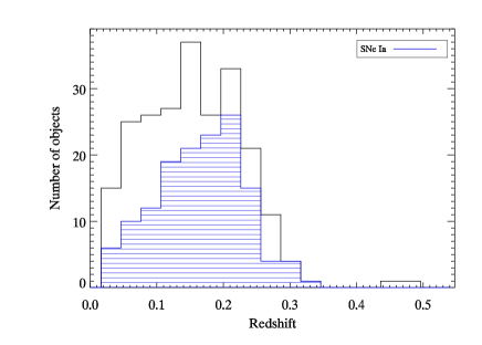
Figure 1: Redshift distribution of the 228 observed objects at the NTT and the NOT with a known redshift. The subset of objects classified as SNe Ia is shown in the striped histogram. The bin size in the plot is 0.03.

The redshift range for all objects observed was $z=$  $0.016$$-$$0.487$, and for the subset of SNe Ia, $z_{SNIa}=$  $0.031$$-$$0.324$.

Our SN Ia sample contains 169 spectra of 141 individual objects, plus 3 likely SNe Ia. In addition, we also obtained 26 spectra of 23 SNe II and 12 spectra of 8 SNe Ib/c. Fourteen spectra were identified as galaxy spectra, which presumably were the result of poor seeing conditions or that the spectra were taken when the SN had faded significantly, becoming much fainter than the host galaxy. These spectra are useful as they provide spectroscopic redshift determination for the photometric sample of SNe. In Section 7 we describe how the spectroscopic typing was performed. The number of spectra and the number of unique objects are summarised in Table 1.

Table 1: Number of spectra and unique objects.

	Spectra	Objects
Total	290	238
with redshift	280	228
SN Ia	169	141
with good LC	127	108
SN Ia?	3	3
SN II	26	23
SN Ib/c	12	8
Not SN	19	16
Galaxy	14	12
Unclassified	61	47

For the first four years of ESSENCE, 55% of the spectroscopically observed objects were identified as SNe Ia, probable SNe Ia or core collapse supernovae (Foley et al. 2009). The corresponding number for the NTT/NOT data set is 72%. The SN fraction obtained depends on the design of the search, the redshift interval, the size of the telescope and the time spent on each supernova target. As two of several telescopes (with different sizes) involved in the follow-up of SDSS SNe, where different targets were assigned to different telescopes, the evaluation of the efficiency is further complicated.

The spectroscopic S/N distribution for the 290 NTT and NOT spectra is shown in Figure 2. Values are computed for 10 Å bins and then averaged over the interval between 4000 and 6500 Å (in observed frame), which is the interval of most interest for SN features.

Figure 2: Distribution of the S/N for the spectra taken at the NTT and the NOT. The S/N is calculated in 10 Å bins and averaged over the interval between 4000 and 6500 Å (in observed frame).

3.1 Lightcurve properties

SDSS multi-band photometry of the objects in our sample and their host galaxies were obtained from $ugriz$ (Fukugita et al. 1996) observations using the method presented in Holtzman et al. (2008). Lightcurves of all confirmed SNe Ia were fitted using SALT (Guy et al. 2005). The same authors have since published a new fitter, SALT2 (Guy et al. 2007). Even though SALT2 in many respects is an improvement, we use the older code since it provides smooth lightcurves which are easy to use for interpolation, e.g. for calculating the photometry of the spectral epoch, to estimate the host galaxy contamination. The fitted parameters are: lightcurve width $s$ (“stretch”), SALT colour $c$, rest-frame peak $B$-band magnitude, and time of $B$-band maximum light. However, 33 SN Ia lightcurves lack either pre- or post-maximum photometry. This leads to bigger uncertainties for the derived lightcurve parameters. In the remainder of this paper, we will refer to these as poor lightcurves. Removing all SNe Ia with poor lightcurves leaves 127 spectra of 108 different SNe Ia.

The epochs of the SN Ia spectra, calculated as the number of days in rest frame from $B$-band maximum light, are listed in Table LABEL:tab:type, and the sample distribution is shown in Figure 3. In the table all epochs calculated from poor lightcurves are marked with a superscript ’$p$’. The uncertainty in the epoch is obtained as either the uncertainty in peak date obtained from SALT or through error simulations, whichever is bigger. The error simulations were performed by randomising the photometry within the error bars and making new SALT fits, after which the spread in the peak date was studied. The epoch errors include the uncertainty in the photometry, but they do not include any potential systematic uncertainties in the SALT fitting procedure.

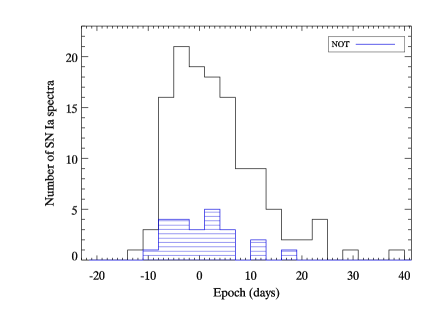
Figure 3: Epoch distribution of the SN Ia spectra observed at the NTT and the NOT, excluding the SNe with poor lightcurves. The un-filled histogram shows the full sample of SN Ia spectra, while the striped histogram shows the subset observed at the NOT. The epoch is defined as the number of days in rest frame since $B$-band maximum brightness, as obtained from the lightcurve. The $127$ spectra are divided into epoch bins with a width of $3$ days.

Figure 4: Distribution of stretch (SALT $s$ parameter) of the SNe Ia observed at the NTT and the NOT, excluding the SNe with poor lightcurves. The mean value is $0.95$ and the standard deviation $0.11$. The 108 objects are divided into bins of size $0.05$. Converting the stretch to $\Delta m_{15}(B)$ following Jha et al. (2006), a mean value of $1.13$ and a standard deviation of $0.22$ is obtained.

The stretch distribution, shown in Figure 4, is similar to the distribution of the Constitution set (Hicken et al. 2009), both regarding the mean value and the shape. The Kolmogorov-Smirnov (K-S) test gives a probability of 35%, which is strong evidence against rejecting the assumption that the two samples of stretch belong to the same distribution.

Figure 5: Distribution of colour (SALT $c$ parameter) for the SNe Ia observed at the NTT and the NOT, excluding the SNe with poor lightcurves. The mean value is $0.08$ and the median $0.07$. The standard deviation is $0.14$. The 108 objects are divided into bins of size $0.05$.

The distribution of colour (SALT $c$ parameter), presented in Figure 5, has a K-S probability of 4% when compared to the distribution of the Constitution sample of Hicken et al. (2009). We conclude that the lightcurve properties of the SNe Ia in our sample are statistically compatible with the SN lightcurves previously used in cosmological analyses.

3.2 Data archive

The spectra are publicly available in electronic format. In addition to the calibrated spectra, a corresponding error spectrum is also provided. Versions of the spectra are available both with and without host-galaxy subtraction. Additional information about the spectra on the website; observing conditions, object type, days since maximum brightness, redshift, etc are available in Appendix A of this paper.

4 Data reduction

The spectroscopic data were reduced using the Image Reduction and Analysis Facility (IRAF) and our own IDL routines. Below follows a step-by-step description of the reduction procedure.

Bias subtraction

Bias frames were taken on every night. No spatial variations were detected so we used the CCD overscan region to subtract the bias.

Flat fielding

The flat fields from the NTT observations had a peculiar feature at the blue end of the spectrum corresponding to wavelengths shorter than roughly 5200 Å (see the left panel of Figure 6). This is an effect from the zeroth order image of the grism which, while being outside the CCD area, still produced a visible glow on the detector. The behaviour was not present in any of the other frames and was removed from the flat fields by fitting a surface over the region.

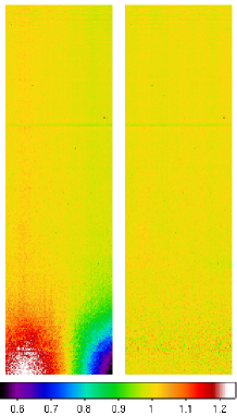
Figure 6: A normalised flat field from the NTT before (left) and after (right) the correction for the zeroth order light was applied. The figure shows only one of the two chips of the CCD. The vertical direction is the dispersion axis and the horizontal direction is the spatial axis. The scales are the same for the two images.

In the right panel of Figure 6, the corrected and normalised flat is shown. Some horizontal lines can be seen in the flat field image around 7600 Å. These are absorption lines due to water vapour and molecular oxygen, and are caused by the long light path inside the instrument. This leads to a variation of the order of 3.5% in the normalised flat.

For a given night of observation, one flat field was constructed for each grism/slit-width combination, which was then used to flat field the 2-D spectral images of the standard stars and the SN candidates.

Spectral extraction

The SN spectra were extracted using the optimal extraction algorithm of Horne (1986). An extraction window was chosen in the spatial direction for a narrow wavelength range and was then traced for all wavelengths. In the cases when the SN was not well separated from the host galaxy, a small spatial extraction window was used to minimise contamination from host-galaxy light. For the sky background subtraction, two small spatial ranges were defined on each side of the SN, and a fitted linear function was subtracted. For extended host galaxies, when the SN light was separated from the core of the host galaxy, this background fit also included host-galaxy light. Any residual host-galaxy light present in the spectra was removed at a later stage in the reduction process (see Section 6.2). When the combination of SN and host galaxy was complex, we experimented with different sizes of extraction apertures and higher orders of background fits, but without any significant improvement in the final result.

Wavelength calibration

For wavelength calibration, spectra of a helium-argon lamp were taken at the NTT and of a helium lamp at the NOT. For each object spectrum, an arc spectrum was extracted with the same centring and trace as the object spectrum. A Chebyshev polynomial of fifth or sixth order was fitted to the identified wavelengths for the arc lamp emission lines. The solution was checked against locations of sky lines. The wavelength solution was then applied to the object spectrum.

Correction for second order contamination

When obtaining spectra over a wide wavelength range in one single exposure, contamination from second order diffraction could lead to an erroneous flux where there is an overlap of the orders. The second order contamination can be circumvented by using a blocking filter for blue light or by ignoring the red end of the spectrum. However, this reduces the wavelength range of the spectrum. Another method is to double the exposure time and divide the observations into a blue part and a red part. However, for faint objects which require long exposure times, this is not desirable. A method has been developed by Stanishev (2007) to correct spectra, obtained at the NOT using grism 4, for second order contamination during the reduction phase. With this method the full spectrum can be used. Observations were made at the NTT using grism 2 to derive the necessary information to correct spectra from that telescope too. To be able to correct for the second order contamination we need to (1) find out the wavelength relation between the first-order spectrum and the second-order spectrum and (2) find the ratio of the efficiencies of the grism for the two orders. The wavelength overlap of the two orders were determined using observations of arc lamps, together with blocking filters. To determine the flux relation between the two orders, bright blue stars were observed with and without order-blocking filters. Szokoly et al. (2004) have developed a similar method.

In extreme cases the second order contamination can be as strong as the flux at long wavelengths. The size and shape of absorption lines at these wavelengths can also be affected. This is illustrated in Figure 7, where two examples of second order corrected spectra are shown, one for each telescope.

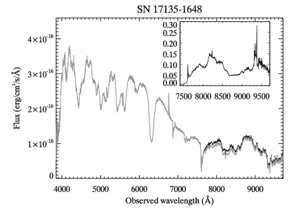
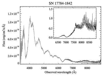
Figure 7: Second order corrections of two SNe, ID 17135 (SN 2006qm) observed at the NTT (top panel) and ID 17784 (SN 2007jg) observed at the NOT (bottom panel). The observed flux is displayed in black and the corrected flux in light grey. The spectra have been flux calibrated. No corrections due to telluric absorption, Milky Way extinction or effects from host-galaxy light have been applied to the spectra shown here. The inset in each panel shows the relative correction with respect to the observed flux.

If the second order contamination is not removed, systematic effects could be introduced since blue SNe are more affected by the contamination than red SNe.

Flux calibration

To correct the object spectra for the wavelength dependent sensitivity of the detector, the spectra were flux calibrated using spectrophotometric standard-stars. For the NTT, the standard stars were observed with a slit width of 5$\aas@@fstack{\prime\prime}$0 and for the NOT with a slit of width 1$\aas@@fstack{\prime\prime}$3. A wider slit width is used to make sure that the seeing does not affect the flux through the slit. All standard stars were observed at parallactic angle, to avoid effects from differential atmospheric diffraction. The standard-star spectra were processed in the same way as the object spectra.

Using IRAF, a sensitivity function was created for each instrument, slit width and observing session (of up to five nights). For the observations at the NOT during September and November 2007, a common sensitivity function was created since few standard star observations could be used. No significant variations with time were seen.

Corrections due to atmospheric extinction were implemented for La Silla and La Palma.

For a significant fraction of the SN observations, the parallactic angle was not used, causing differential slit losses due to atmospheric refraction. This problem will be discussed in detail in Section 5.

Telluric removal

The spectra have been corrected for telluric absorption. Using standard-star observations the telluric absorptions were isolated and then combined into one telluric spectrum for each slit width and night of observations. The SN spectra were then corrected through division of a scaled telluric spectrum. The scale factor was determined as the optimal weight for removing any telluric absorption near 7600 Å. This is the dominant telluric region, while not containing any interesting SN features for objects in our redshift range. In some cases no weight could be found such that the telluric spectrum obtained during the same night could remove the telluric feature. If another telluric spectrum obtained in close connection to the SN spectrum could do the matching, this was used instead. Some spectra could not be corrected perfectly using any telluric spectrum. The increased uncertainty in the spectra due to possible un-corrected telluric absorption was estimated by calculating the deviation from a spline fit through the 7600 Å region, after correction. This error was then added to the SN error-spectrum.

Correction for dust extinction in the Milky Way

The spectra were corrected for dust extinction in the Milky Way using $R_{V}=3.1$ and the colour excess $E(B-V)$ from Schlegel et al. (1998). The extinction was assumed to follow the Cardelli et al. (1989) extinction law modified according to O’Donnell (1994). According to Schlegel et al. (1998), the uncertainty on $E(B-V)$ is of the order of 16%. The errors due to the uncertainty in $R_{V}$ and the uncertainty in the extinction law was found to be of less importance. The wavelength-dependent errors from the Milky Way correction were added in quadrature to the existing error spectrum.

5 Differential atmospheric refraction and slit losses

Differential atmospheric refraction (DAR) occurs when an observed image is spread out with wavelength along the direction toward the horizon due to the wavelength dependence of the refraction index of air (see e.g. Filippenko 1982; Cuby et al. 1998). As a result, objects centred on the slit for one wavelength, may be partially or even fully outside the slit for shorter and longer wavelengths. The effect can be minimised by (1) observing at a low airmass and (2) rotating the slit to the parallactic angle, where the slit is parallel to the direction of the atmospheric refraction, i.e. normal to the horizon. Other factors affecting the differential slit loss are: slit width, seeing, morphology of the observed object, spectral coverage and the wavelength(s) for which the object is centred.

The spectroscopic observations of SNe presented in this paper were typically not made at parallactic angle. Instead, the slit orientation was most often chosen to simultaneously give a spectrum of the host galaxy. The differential atmospheric refraction (in arcseconds) for a certain wavelength with respect to a reference wavelength was estimated using the formulae by Owens (1967). The reference wavelength is the wavelength with which the SN had been centred on the slit. To calculate the fraction of the flux within the slit for each wavelength we modelled the SN flux with a Gaussian distribution using the seeing at the time of observations. In Figure 8, we show one of the observed spectra with an insignificant host-galaxy contamination and a severe differential slit loss. The spectrum is shown together with a SN Ia template from Hsiao et al. (2007) (which we from now on will refer to as Hsiao templates) in its original form as well as affected by the estimated differential slit loss. The slit loss affected template is a much better fit to the observed spectrum. The estimated slit loss at very short wavelengths is exaggerated, which seems to be true for a large fraction of the theoretically calculated slit loss functions. In most cases such a direct comparison cannot be made due to the complex interplay of host-galaxy contamination and slit loss effects.

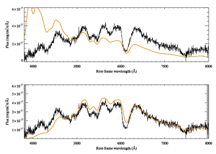
Figure 8: The observed spectrum of ID 16287 (SPID 1449) 2 days past maximum brightness is shown in black together with the Hsiao template at the same epoch in orange (upper panel). In the lower panel the Hsiao template has been multiplied with the theoretically calculated differential loss due to the atmospheric refraction.

In Table LABEL:tab:qual we indicate the estimated effect from the differential atmospheric refraction on the spectra at an observed wavelength of 4000 Å. It should be noted that this is only a rough estimate of the differential slit loss since many simplifications are used in the calculations and the centring over the slit was not perfect. For a non-negligible fraction of the NTT/NOT spectra, the differential slit loss is severe at short wavelengths. This is due to large airmasses and large differences between the observing angle and the parallactic angle. The median value of the airmass of the observations is 1.4, with 39% of the observations having an airmass larger than 1.5. Large airmasses were unavoidable because of the position of the SDSS SN fields relative to the NTT and the NOT sites, during the observing season. Deviations from observations at the parallactic angle were also fairly large: nearly half of the spectra (46%) were observed with 45^∘ or more from the parallactic angle. The centring of the objects on the slit was done at wavelengths above 4600 Å, typically at 6500 Å.

A polynomial multiplier is included in the host-galaxy subtraction to account for the differential slit loss effects. However, these empirically determined corrections differ from the theoretically estimated functions described above since the polynomial also accounts for reddening.

6 Host-galaxy contamination

A large fraction of the obtained SN spectra are contaminated by galaxy light. We present below an estimation of the galaxy contamination in the spectra from photometry and a description of the host-galaxy subtraction method applied to the data.

6.1 Estimating the degree of host-galaxy contamination

The host-galaxy contamination in the observed spectra was estimated using multi-band SDSS photometry. To obtain an estimate of the galaxy light in the slit, the measured photometric surface brightness of the galaxy at the position of the SN was scaled to the area defined by the slit width times the width of the spectral extraction window. The expected SN flux in the observed spectra was calculated using the SDSS lightcurve, interpolated to the night the spectrum was taken. For objects where good lightcurve fits were available, these were used for the interpolation. The amount of SN flux through the slit was estimated by modelling the SN flux as a Gaussian distribution with the width determined from the seeing. The seeing variations between the different filters were estimated following Schroeder (1987) ($\propto\lambda^{-0.2}$). In Table LABEL:tab:qual, the estimated contamination in the $g$-band (observed frame) for each observed spectrum is listed. The contamination values are rough estimates and they are more likely over estimated since we assume that all galaxies are extended over the whole extraction window. Out of the spectra, 31% have an estimated contamination less than 20%. The cases where extrapolation of the lightcurve was necessary are marked with a superscript of ’$e$’ in the table. These values should be considered less reliable.

6.2 Host-galaxy subtraction

In the past, several different techniques have been used to subtract the host-galaxy contribution from observed spectra, such as $\chi^{2}$ based template fitting using the spectrum of the actual host galaxy or templates, either varying the contamination level or estimating it from photometry (e.g. Howell et al. 2005; Ellis et al. 2008). For the vast majority of the NTT/NOT spectra, no good quality spectra of the host galaxy at the location of the SN were accessible at the time of the work and thus a $\chi^{2}$ based fitting using a real galaxy spectrum was rejected. To model the galaxy, principal component analysis (PCA) was chosen over template spectra. A similar method has also been used by Zheng et al. (2008). There are also host-galaxy subtraction methods which separate the two components, SN och galaxy, in the two dimensional spectrogram (Baumont et al. 2008). However, this requires higher resolution of the data than that of the NTT/NOT data set.

For the NTT/NOT data set a number of different methods to subtract host-galaxy light from spectra were explored. We found the most stable method to be a principal component analysis based subtraction of galaxy eigencomponent spectra. For a large fraction of the moderately contaminated spectra (10-70% contamination in the $g$-band) we found this method to yield good results.

It should be noted that some part of the host-galaxy light, at least for host galaxies with larger spatial extent on the CCD, were removed during a linear background fit in the reduction of the spectra. For these spectra the host-galaxy contamination that was fitted thus were the residuals from the reduction.

An additional difficulty in the host-galaxy subtraction was that a large fraction of the NTT/NOT spectra were not observed at parallactic angle (see Section 5), and were thus affected by a wavelength dependent flux loss.

In the PCA-based subtraction method described here, SN templates were used. A potential worry is that the usage of templates constructed from normal low-redshift SNe might affect the outcome of the subtraction. This concern and other concerns are addressed in Section 6.5.

PCA-based galaxy subtraction

The spectral energy distribution (SED) of the host galaxy was estimated through minimising the difference between the observed spectrum and a combination of a SN template and a set of galaxy eigencomponent spectra. The minimisation can be described with the formula

$$f_{\rm{fit}}(\lambda)=a_{0}s(\lambda)\cdot f_{\rm{SN}}(\lambda)+\sum_{i=1}^{n}a_{i}g_{i}(\lambda),$$ (1)

where $f_{\rm{SN}}$ is the SN template, $g_{i}$ the galaxy eigencomponent spectra, $s$ is a second degree polynomial and, $a_{i}$ weights which are fitted in the subtraction.

The galaxy eigencomponent spectra were created in a PCA analysis of 170 000 SDSS galaxy spectra (Yip et al. 2004). The three most dominant eigenspectra have been shown to describe 99% of all galaxies. The fit can be made arbitrarily complex through the inclusion of more galaxy eigencomponent spectra (to the existing three), but this extension was not used in the final studies since the fits did not improve significantly while the computational demands increase drastically. In the fit we included the constraint that the total galaxy flux must be positive.

For the SN template in the fit we tried all Hsiao templates with epochs $\pm$5 days from the spectral epoch as obtained from the photometric lightcurve. We also included templates of more peculiar SNe, SN 1991bg and SN 1991T (Nugent et al. 2002), to study how well the Hsiao templates worked and to, possibly, find peculiar SNe in our sample. None of our spectra were well fitted with the SN 1991bg template (there will be a bias against such objects due to their faintness). Some spectra had better fits with a SN 1991T template. The difference in the features sizes between the subtraction with the Hsiao template and the SN 1991T template was small in these cases.

To the SN template a second degree polynomial was multiplied which was introduced to account for reddening (e.g. due to host galaxy dust extinction) and differential slit loss effects. During observations, the object was centred on the slit in the red part of the spectrum, and thus differential slit losses due to atmospheric refraction (see Section 5), when present, predominantly affects the blue end (as would extinction). The second degree polynomial was fixed to have $s\equiv 1$ at the wavelength $\lambda_{1}=6600$ Å and $s<1$ for all other wavelengths. The value of $\lambda_{1}$ was chosen to correspond to the wavelength where most spectra were centred on the slit. The function describing the differential slit loss is asymmetric around this wavelength, but since the fit during host-galaxy subtraction was only made between 4000 Å and 6000 Å, the behaviour of the slit loss function at longer wavelengths did not affect the fit. The polynomial was only multiplied with the SN SED, and not with that of the galaxy. The reason for this was that since galaxies are not point sources, they are less affected by differential slit losses. A separate polynomial could be modelled for the fitted galaxy, but this would be both hard to evaluate and too computationally demanding, considering the small effect. A test was performed where the same polynomial was added both to the galaxy and the SN, but this did not improve the quality of the fits.

The code for the PCA-based host-galaxy subtraction has only been applied to SNe Ia with known redshifts and a good lightcurve (photometry both before and after peak brightness). Two sample subtractions for one moderately and one highly host-galaxy contaminated spectrum can be seen in Figures 9 and 10.

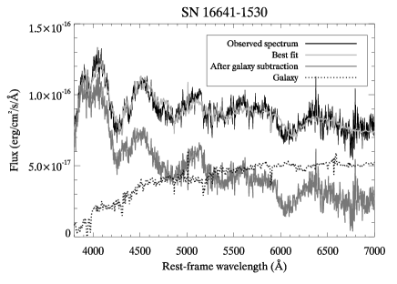
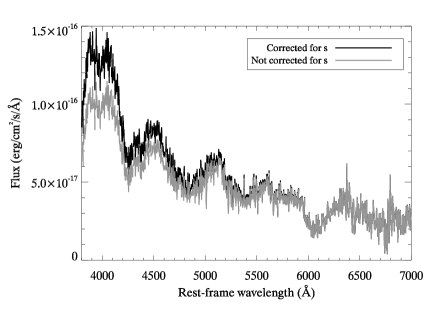
Figure 9: The PCA-based host-galaxy subtraction for ID 16641 (SN 2006pr) at $z=$ 0.132. Left panel: The observed spectrum (black) is plotted together with the best fit (light grey). The galaxy template of the best fit is shown as a dotted line. The grey line shows the SN spectrum after subtraction of the estimated galaxy light. Right panel: The (host subtracted) SN spectrum is shown with and without correction for the wavelength dependent flux loss described by $s$ (black/grey). The host galaxy contamination estimated from photometry (40%) agrees well with the fraction of host galaxy light indicated by the subtraction. The expected differential slit loss estimated following Section 5 (30% at 4000 Å) also seems close to what the best fit in the host-galaxy subtraction indicates (compare the curves at 4000 Å in the right panel).

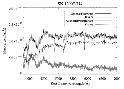
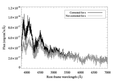
Figure 10: The PCA-based host-galaxy subtraction for the highly contaminated ID 12907 (SN 2006fv) at $z=$ 0.132. Left panel: The observed spectrum (black) is plotted together with the best fit (light grey). The galaxy template of the best fit is shown as a dotted line. The grey line shows the SN spectrum after subtraction of the estimated galaxy light. Right panel: The (host subtracted) SN spectrum is shown with and without correction for the wavelength dependent flux loss described by $s$ (black/grey). The host galaxy contamination estimated from photometry (80%) agrees well with the fraction of host galaxy light indicated by the subtraction. The expected differential slit loss, see Section 5, (30% at 4000 Å) also seems compatible to what the best fit in the host-galaxy subtraction indicates (compare the curves at 4000 Å in the right panel).

6.3 Host-galaxy simulations

Set-up

To evaluate the subtraction methods, a large number of simulated “fake” spectra were constructed and run through the subtraction pipelines. Each fake spectrum was constructed through a combination of a SN and a galaxy spectrum, redshifted to some distance. Reddening and differential slit loss were added to the SN spectrum. Finally, noise was added. All parameters (redshift, spectral epoch, host-galaxy contamination, reddening, differential slit loss) were drawn from distributions that match the NTT/NOT data set. In constructing these fake spectra we avoided all templates/functions that were used in the host-galaxy subtraction pipeline (as this would make the fit trivial). More details about the different components of the fake spectra are given below:

• Supernova spectra
  All SN spectra that were used to construct fake spectra have high S/N and low host-galaxy contamination. Their epochs are similar to the ones of the NTT/NOT spectra. Seven different spectra of normal SNe Ia were used: six of SN 2003du (epochs $-$6, $-$2, 4, 9, 10, 17) (Stanishev et al. 2007) and one of SN 1998aq at peak brightness (Branch et al. 2003). Furthermore, two spectra of the sub-luminous SN 1999by (epochs $-$5 and 3) (Garnavich et al. 2004) were used and two of the peculiar and luminous SN 1999aa (epochs $-$5 and 0) (Garavini et al. 2004).

• Reddening
  Reddening was added to the SN spectrum using the Cardelli et al. (1989) extinction law with a total-to-selective extinction ratio $R_{V}$ of 2.1 and a colour excess $E(B-V)$ drawn from the distribution of $E(B-V)$ obtained from the NTT/NOT lightcurve fits. The lower value of $R_{V}$ compared to the Milky Way average was chosen to agree with the values often derived when looking at SNe Ia (see e.g. Altavilla et al. 2004; Nobili & Goobar 2008).

• Galaxy spectra
  In a first simulation series, four galaxy templates of varying type (elliptical, S0, Sa and Sb) from Kinney et al. (1996) were used together with three real galaxy spectra (host galaxy spectra for ID 7527, 13840 and 15381) observed at the NTT at the same time as the SN spectra presented here. The contamination level was randomly chosen between 0 and 70% for the $g$ band. These simulations were later extended in a second series, where 50 randomly chosen SDSS galaxy spectra were used. Figures displayed here are based on the first run, but results are very similar when including the second set of galaxy spectra.

• Redshifts
  The object redshift was randomly drawn from the NTT/NOT redshift distribution.

• Differential slit loss
  To the SN spectra we multiplied functions modelling the expected differential slit loss due to atmospheric refraction for typical NTT/NOT observing conditions (see Section 5). These effects range from insignificant to severe. The slit loss functions are applied to the SN spectra but not to the galaxy spectra.

• Noise
  An S/N value was randomly chosen from the NTT/NOT spectral S/N distribution. Poisson noise was then added to the spectrum until the target S/N was achieved. The shape of the Poisson noise was determined as a linear combination of the input spectrum and a randomly chosen NTT/NOT sky spectrum. The linear combination was determined such that the highest S/N value in the NTT/NOT sample corresponded to no contribution from sky noise, the lowest S/N corresponded to complete dominance by sky noise and intermediate values to a combination of the two error sources. Simulations were done both with and without noise. As can be expected, added noise increased the dispersion around the true solution, but no significant bias effects were detected.

For the simulations without noise, 5000 fake spectra were constructed and about twice as many for the simulations with noise.

Evaluation of the host-galaxy simulations

The simulations can be evaluated using a range of different tests. For all fake spectra we compared the input SN and galaxy spectra with the SN and galaxy as estimated by the host-galaxy subtraction pipeline. In Nordin et al. (2010) we study how spectral indicators are affected by the host-galaxy subtraction as a function of contamination level. A more direct way of evaluating subtractions is to compare the input contamination with what is obtained from the subtraction output. In Figure 11 we show how the difference between input and fitted output contamination varies with input contamination (in the $g$ band). The dispersion is largest for low contamination levels. When studying the contribution from different SN templates, it is found that for contamination levels roughly below 20%, some SN templates yield a small offset. This offset has its origin in a combination of two effects: First, some of the SN templates most likely contain some host galaxy light. This would be seen as a slight bias for low contamination levels, but should thus not be interpreted as a bias of the host subtraction method. Second, a bias can occur if the SN spectrum is imperfectly matched to the Hsiao template. The offset decreases with contamination level. For objects with very low contamination it can thus be advantageous not to subtract the estimated host galaxy light since the correction likely is smaller than the uncertainty in the correction. No trend with galaxy template or slit loss function could be seen.

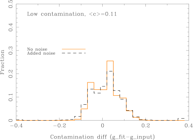
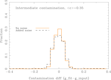
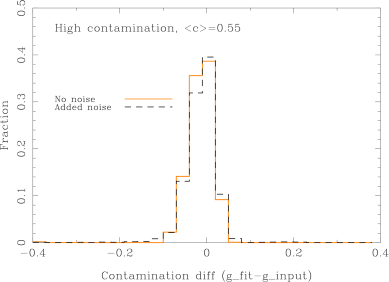
Figure 11: The difference between the $g$-band host-galaxy contamination that was introduced in the construction of fake spectra ($g\_{\rm{input}}$) and the contamination that was obtained during host-galaxy subtraction ($g\_{\rm{fit}}$) for three different bins in $g\_{\rm{input}}$. The mean contamination for each bin is given in the respective panel as $<c>$. The contamination was calculated as the percentage of the total flux in the observed SDSS $g$ band which comes from the galaxy. The solid histogram corresponds to simulations without added noise while the dashed line corresponds to where noise is added. The dispersion is largest for small input contaminations. The number of outliers increase from 0.9% to 2% when noise is added.

When noise is added to the fake spectra, the number of failed subtractions increase, from 0.9% to 2%. These failures are usually evident through a visual inspection of the subtraction. The percentage agrees with what is seen when evaluating subtractions of real SNe. These events likely correspond to random noise mimicking host galaxy or SN features.

6.4 Alternative methods

Several other host-galaxy subtraction methods were tried: varying the galaxy eigenspectra (their number and source), varying the limitations of the eigenspectra, using a large set of SN templates and using SDSS photometry to fix the fraction of galaxy light as well as the proportions of different galaxy eigenspectra. These alternative methods were found to be either less stable than the method above or equivalent (but involving more computational effort). It should be noted that for some individual SNe Ia, an alternative method might perform better. Alternative host-galaxy subtractions of spectra can be provided upon request.

6.5 Discussion on the host-galaxy subtraction

The host-subtraction method is not successful for all NTT/NOT SNe, especially for very faint or contaminated cases. It is, however, not obvious how to judge when a subtraction does fail. Both visual inspection and $\chi^{2}$ tests only indicate how well the subtracted spectrum match the local template, and can thus not be trusted to completely specify which subtractions succeed.

Some of the main worries with the subtraction technique used here are: (i) the observed SNe could differ from the local SN templates used e.g. if it is a peculiar type; (ii) the true galaxy contribution to the spectrum could be badly described by the use of galaxy eigencomponent spectra since the complete galaxy is not recorded in the slit; and (iii) the approximation of slit loss and reddening with a polynomial (applied to the SN but not to the galaxy SED) is a simplification. Regarding the first point, object typing was also performed prior to galaxy subtraction, which means that any truly odd SN would have been spotted at this stage unless it is heavily contaminated by galaxy light. Furthermore, the SN template is only used in the choice of what galaxy spectrum to remove and the number of bins used in the fit is large compared to the number of parameters which are fitted and thus the risk of affecting the spectrum severely is small. Regarding the second point, the three most dominant eigenspectra have been shown to be able to describe 99% of all galaxies (Yip et al. 2004), which means that they should be sufficient to describe our host galaxies as well. The third point, as well as the host-galaxy subtraction code in general, was tested through an extensive number of simulations as described in Section 6.3. The host-galaxy subtraction does fail in roughly one percent of all runs, but these cases usually fail completely, yielding unphysical results, and are thus easily detected.

In Nordin et al. (2010) we further test the host-galaxy subtraction code, by examining the effects on spectral features, in particular on pseudo-equivalent widths. We also compare the trends of pseudo-equivalent widths for the full sample with the subsample of spectra with low host-galaxy contamination and conclude that no bias is introduced.

7 Typing

The object spectra have been typed using SNID (SuperNova IDentification; Blondin & Tonry 2007), version 5.0. This algorithm cross-correlates the unknown spectrum against a set of template spectra. The template database includes SN spectra of different types and ages as well as non-SN spectra of galaxies, AGNs and stars. The redshift of the object can either be varied or fixed. In this version of the code, SNID distinguishes between the following types and subtypes (within parenthesis): Ia (Ia-norm, Ia-91T, Ia-91bg, Ia-csm, Ia-pec), Ib (Ib-norm, Ib-pec, IIb), Ic (Ic-norm, Ic-pec, Ic-broad), II (IIP, II-pec, IIn, IIL), Not-SN (AGN, Gal, LBV, M-star). The Ia-pec group consists of SNe of the type SN 2000cx and SN 2002cx. As a figure of merit for the classification we have used the rlap parameter (see Blondin & Tonry (2007) for a definition). A good correlation was considered to be obtained if rlap was greater or equal to five. Following Foley et al. (2009) we made four runs with SNID to determine the type, subtype, redshift and age, one at a time. This was done in the following manner:

• First we attempted to determine the type. A type was identified if more than 50% of the templates with a good correlation belonged to this type and the best-match SN-template (highest rlap value) had the same type. When the redshift of the SN was known, we restricted the redshift range of SNID to this redshift ($\pm 0.02$).

• If it was possible to determine the type, we continued with trying to determine the subtype. We fixed the type and the redshift (if it was known). A subtype was considered to be identified if more than 50% of the templates with a good correlation belonged to a specific subtype and the best-match spectrum was of the same subtype.

• Regardless if a subtype was identified or not, we determined the best-fit redshift. We now locked SNID to the templates of the identified type or subtype and fitted for the redshift. The SNID redshift was defined as the median of the redshifts belonging to templates with a good correlation. The error was given as the standard deviation.

• To determine the age, the type was fixed to the identified type or subtype. If we had a spectroscopic redshift, we fixed the redshift in SNID to this value. Otherwise we used the value obtained in the step before with a redshift error of 0.02. The SNID age was then defined as the median of all ages belonging to templates with a good correlation. The error of the age was given as the standard deviation of these values.

If the determined type and redshift were inconsistent in that the preferred type was an M-star or an LBV, while the redshift was too high for such an object to be detected, the type was set to unknown.

A problem with this method is that the composition of the template database affects the possibilities to detect different types. The SNID database has few spectra of core-collapse SNe and peculiar SNe Ia which makes these objects harder to type. It is also less effective for low S/N spectra than for those with high S/N.

The outcome of the SNID analysis is presented in Table LABEL:tab:type. The typing for each spectrum is presented in the column NTT/NOT type. When the type was determined using the host-galaxy subtracted spectrum, this is marked in the column for notes with the addition of an $s$. In some cases a spectrum only had a good match using SNID with one particular object in the database. In these cases we have marked this in the table. When no type could be determined this is marked with “$-$”.

The consistency in typing when several spectra of the same object existed was good. If a type could be determined, the same type was always obtained. In some cases, one of the spectra was left without a type due to, for example, noise making the classification difficult or it was classified as a galaxy, due to the faintness of the SN at that epoch.

After a visual inspection of the spectra, the typing from SNID was changed for $36$ spectra. The majority of these, $20$, could not be typed by SNID but could be clearly typed by visual inspection. There was also a group of spectra, $11$, which had been typed by SNID, but with only few well matched template spectra, and, in the visual study, they were found to be of such low quality that it was not possible to say with certainty what the type was. Three spectra had a type which was changed, one from a Ib to a Ib/c and two from a Ia to a possible Ia. There were also two cases where the type was kept, but the subtype was removed. The spectra whose type was changed following the visual check are marked with a $v$ in the column for notes in the table.

The NTT/NOT objects also have an SDSS typing based on the NTT and the NOT spectra in combination with spectra taken at other telescopes as a part of the SDSS-II SN Survey. This type is presented in Table LABEL:tab:type under the column SDSS type. Due to the faintness of the SN in some spectra, not all NTT and NOT spectra could be typed and some were typed as galaxies, while the overall SDSS typing is a SN, based on spectra at other epochs from other telescopes.

In Figure 12 the redshifts obtained from SNID are compared with the SDSS object redshifts from Zheng et al. (in preparation), which mainly come from the SDSS DR7 catalogue and measurements of galaxy lines in spectra obtained as a part of SDSS-II. Some are determined from SN features (see Section 3).

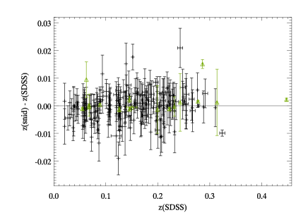
Figure 12: A comparison of the SDSS object redshifts with the redshifts determined using SNID. The vertical error bars show the uncertainty in the SNID redshifts. The horizontal error bars show the uncertainty in the SDSS object redshifts. In most cases these are too small to be visible. All redshifts determined from SN features have an error of at least 0.005. The RMS of the distribution is $0.005$ (with a negligible bias). SNID redshifts which are calculated using less than five well matched spectra are marked with green triangles.

There is a good agreement between the SNID redshifts and the SDSS redshifts, with a dispersion of $0.005$ and a negligible bias. No dependence with redshift is detected.

In Figure 13, the ages of the spectra as estimated with SNID are compared with the ages obtained from the lightcurves, $({\rm{MJD}}_{\rm{spec}}-{\rm{MJD}}_{\rm{max}})/(1+z)$, for the spectra which we have classified as SNe Ia.

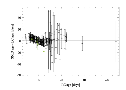
Figure 13: A comparison of the age obtained using SNID and the age obtained from the lightcurve fit using SALT. The age is here defined as the number of days in rest frame since $B$-band maximum. SNID ages which are calculated using less than five well matched spectra are marked with green triangles.

A dispersion of $4$ days was obtained. It should be noted that for young SNe, SNID generally estimates an older age compared to the SALT lightcurve fit and that the errors in the age from SNID are typically overestimated, especially at later epochs. This was also pointed out by Blondin & Tonry (2007). Since the estimated age error bars are symmetric (estimated as the standard deviation) and in many cases overestimed, there will be some cases where the minimum allowed age (from the error bar) will be unphyically low. We have not used any prior on the age from the lightcurve, which cause the large error bars and the bias in the epoch estimates at early epochs. It should be noted that the error bars, in a few cases, also could be underestimated. This occurs when the observed spectrum is only well fitted with few template SNe and these template epochs do not sample all different ages of a SN. One example is ID 16838 which is only well fit by spectra in the library of SN 1998S. For one spectrum (ID 20142), no error was estimated since only one template spectrum could fit the observed spectrum. We also test the hypothesis that the evolution of spectral features scale with the stretch factor, by multiplying the age obtained from SNID with $s$. The bias is slightly improved, while the spread increases.

8 Some special objects

Possible non-normal SNe Ia

Using SNID we find that the spectrum of ID 16333 (SN 2006on) is only well described by spectra of SN 1991T. The fit with SN 1991T at 5 days before maximum brightness is shown in Figure 14.

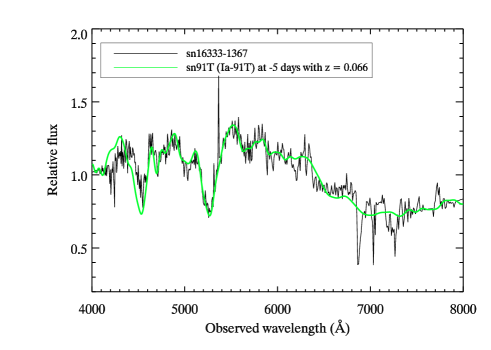
Figure 14: SNID fit for ID 16333 (SN 2006on) with a SN 1991T template at 5 days before lightcurve maximum.

The peak brightness of the SN is well constrained by the lightcurve fit (the stretch and colour less so) and we find a peak $B$ absolute magnitude of $-$19.06. The obtained stretch was 0.94 and the SALT $c$ colour 0.19. Correcting the peak magnitude for stretch and colour, following $M_{B}+\alpha(s-1)-\beta c$, gives a peak magnitude of $-$19.6, which is consistent with a SN 1991T-like SN.

The spectrum of ID 17176 (SN 2007ie) has strong indications of being a SN 2002cx-like object. Using SNID, the spectrum is best fit with a spectrum of SN 2002cx. However, also other classes of SNe Ia give sufficiently good fits to the spectrum, when allowing for a variation of 0.02 in redshift. In Figure 15, some of the SNID fits with different template spectra are shown.

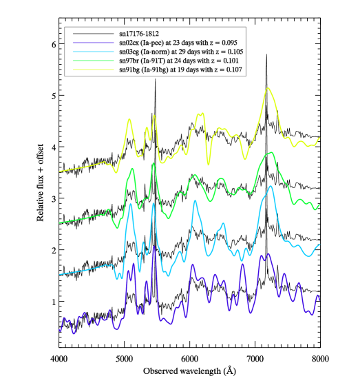
Figure 15: The observed spectrum of ID 17176 (SN 2007ie) in black together with different template spectra as indicated in the legend. In the fit, the redshift has been fixed to 0.0935, the redshift of the object as obtained from SDSS DR7, with an allowed variation of 0.02. The fit with the spectrum of SN 2002cx gives the best match and the closest redshift compared to the one of the host galaxy.

The spectrum of SN 2002cx is a better fit to the double peaks at an observed wavelength of 5100 Å and 6100 Å than the other spectra (normal SN Ia, SN 1991T and SN 1991bg). Furthermore, the fit with the spectrum of SN 2002cx gives a better match with the redshift of the SN as obtained from SDSS DR7. If we reduce the allowed redshift range in SNID to $\pm 0.01$, SNID identifies the spectrum as a SN 2002cx-like object. By comparing the spectrum with the ones by Sahu et al. (2008) of SN 2005hk, which also is a SN 2002cx-like SN, we identify absorption by Fe ii $\lambda$5018, Fe ii $\lambda$5535, Fe ii $\lambda$6149 and Fe ii $\lambda$6247. The velocities in our spectrum for these lines are lower by 7$-$35% compared to a spectrum of SN 2005hk at 24 days past peak brightness. Compared to the spectrum at 38 days past peak, the velocities varies from being lower by 26% to being higher by 9%. The lightcurve, in this case, is not well constrained due to lack of photometry before maximum brightness. The best-fit absolute peak magnitude in the $B$-band from SALT is -18.2, which is comparable to what is expected for SN 2002cx-like objects.

ID 19149 (SN 2007ni) is best fit with a SN 1991T-like spectrum according to SNID. It also has great similarities with SN 2002cx-like and SN 2000cx-like spectra, but not with spectra of normal SNe Ia. Comparisons from SNID with different templates are shown in Figure 16.

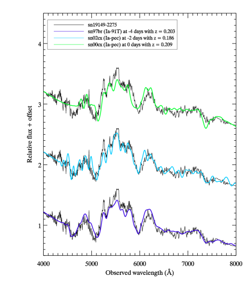
Figure 16: The SNID fit of ID 19149 (SN 2007ni) with the observed spectrum in black and different template spectra in colour as indicated in the legend.

The lightcurve fit is well constrained and the obtained absolute peak magnitude in $B$ is $-$19.47, which is somewhat brighter than a normal SN Ia. We could thus exclude an SN 2002cx interpretation. The stretch and SALT $c$ colour are 1.04 and 0.09, respectively.

ID 20978 (SN 2007rl) is best fit in SNID with a spectrum of SN 2000cx. However, due to its high redshift, it is well fitted by many different templates. The peak brightness is well constrained by the photometry, while the stretch and colour are less so due to few observations past peak brightness. The absolute peak $B$ band magnitude is $-$19.6.

Possible SNe IIn

In the spectral fitting we find that the spectrum of ID 16838 is best fit with a SN IIn, similar to SN 1998S. Another potential SN IIn is ID 16668 (SN 2006pu).

Stellar tidal disruption event

The object with SDSS identification 17237 has been suggested to be a stellar tidal disruption event (van Velzen et al., in preparation), an event where a star passes close to a supermassive black hole in the centre of the galaxy without being completely destroyed.

9 Summary

We have presented observations and reductions of 290 spectra observed at the NTT and the NOT as a part of a programme to classify SNe discovered by the SDSS-II. The selection procedure, the observing strategy and the reductions have been performed in a coherent and well documented manner. The spectra have been corrected for telluric absorption. Objects classified as SNe Ia were processed through a host-galaxy subtraction pipeline. The host galaxy SEDs were estimated using a PCA-analysis where the difference between the observed spectrum and a combination of a SN template and galaxy eigencomponent spectra were minimised. A polynomial was multiplied to the SN templates to account for reddening effects as well as differential slit loss due to atmospheric refraction. The host-galaxy subtraction pipeline was evaluated using extensive simulations mimicking the distribution of parameters for the NTT/NOT data set. Furthermore, careful estimates of uncertainties have been made, thus making our data well-suited for systematic studies.

The spectra were classified using SNID, a template-matching algorithm. The age of the spectra estimated using SNID was compared to the age obtained from the lightcurve, in the case of SNe Ia, and was found to agree well, with an age dependent bias of a few days and an overall dispersion of $4$ days. The typing was revised using visual inspection and changed in some cases; typically when the SNID classification was unreliable due to few matched spectra or when the spectrum could be typed by visual inspection but not with SNID.

In total, 207 spectra of 172 different confirmed SNe were obtained at the NTT and the NOT for the SDSS-II SN program. Out of these, 169 are SN Ia spectra, and some of these (the ones which will survive the strict cosmology lightcurve cuts) will be part of a larger sample to be included in the three year SDSS-II SN Hubble diagram. Four potential peculiar SNe Ia were identified from their spectra. ID 16333 (SN 2006on) and 19149 (SN 2007ni) are potential SN 1991T-like objects, while ID 17176 (SN 2007ie) is a potential SN 2002cx object. ID 20978 (SN 2007rl) is identified as a peculiar SN Ia using SNID, but due to its high redshift, it is difficult to determine a subtype. The sample also includes 26 spectra of 23 SNe II and 12 spectra of 8 SNe Ib/c.

The reduced spectra are made public together with the estimated uncertainty for each wavelength. For the subsample of SNe Ia, host-galaxy subtracted spectra are provided. All this data is accessible from the webpage: http://www.physto.se/$\sim$linda/spectra/nttnot.html

Appendix A Tables

Table 2: Information about the observations.

ID	SPID	IAU	Telescope	Slit Width (arcsec)	Exposure Time (s)	Airmass	Seeing (arcsec)
12778	692	2006fs	NTT	1.0	1000	1.16	1.1
12779	693	2006fd	NTT	1.5	1000	1.27	1.2
12781	680	2006er	NTT	1.5	1800	1.14	1.9
12782	681	2006fq	NTT	1.5	1000	1.27	1.6
12820	711	2006fg	NTT	1.5	600	1.41	1.8
12842	682	2006ez	NTT	1.5	800	1.14	1.5
12843	727	2006fa	NTT	1.0	1000	1.15	0.8
12844	684	2006fe	NTT	1.0	2000	1.21	1.6
12853	685	2006ey	NTT	1.5	1000	1.17	1.1
12855	716	2006fk	NTT	1.5	2000	1.25	2.0
12856	695	2006fl	NTT	1.5	2197	1.38	1.5
12860	688	2006fc	NTT	1.5	1000	1.16	1.6
12874	689	2006fb	NTT	1.5	2400	1.20	2.5
12898	712	2006fw	NTT	1.5	600	1.35	1.5
12907	714	2006fv	NTT	1.5	600	1.21	1.6
12927	690	2006fj	NTT	1.5	1800	1.25	2.5
12928	686	2006ew	NTT	1.0	2000	1.20	1.2
12930	687	2006ex	NTT	1.5	1000	1.16	1.4
12947	691		NTT	1.5	1500	1.36	1.7
12950	700	2006fy	NTT	1.0	600	1.19	1.1
12950	1055	2006fy	NTT	1.0	600	1.37	1.1
12978	701		NTT	1.5	1800	1.59	3.0
13005	702	2006fh	NTT	1.5	2000	1.14	2.0
13025	761	2006fx	NTT	1.0	1200	1.24	0.8
13044	724	2006fm	NTT	1.0	900	1.19	1.0
13044	1062	2006fm	NTT	1.0	1200	1.60	1.2
13045	734	2006fn	NTT	1.0	1000	1.41	1.7
13046	726		NTT	1.0	1500	1.46	1.4
13070	736	2006fu	NTT	1.0	2000	1.19	0.9
13072	723	2006fi	NTT	1.0	1500	1.30	1.7
13135	739	2006fz	NTT	1.0	1200	1.19	1.7
13135	998	2006fz	NTT	1.0	600	1.26	1.2
13174	766	2006ga	NTT	1.5	1000	1.48	1.6
13195	764	2006fo	NTT	1.0	300	2.04	1.7
13195	983	2006fo	NTT	1.0	900	1.66	1.7
13195	1458	2006fo	NTT	1.0	900	2.00	0.8
13355	1003	2006kh	NTT	1.0	900	1.47	1.4
13376	1002	2006gq	NTT	1.0	1200	1.36	1.4
13376	1106	2006gq	NTT	1.0	1800	1.66	1.4
13577	1000	2006kg	NTT	1.0	900	1.62	1.7
13796	1058	2006hl	NTT	1.0	900	1.51	1.3
13894	1039	2006jh	NTT	1.0	1800	1.35	1.1
14157	1040	2006kj	NTT	1.0	1800	1.26	1.0
14279	1459	2006hx	NTT	1.0	900	1.87	0.9
14318	1594	2006py	NTT	1.0	900	2.47	1.0
14318	1653	2006py	NTT	1.0	600	1.99	1.6
14318	1713	2006py	NTT	1.5	1800	1.77	2.3
14437	1061	2006hy	NTT	1.0	900	1.43	1.2
14450	991	2006kn	NTT	1.0	1800	1.21	1.0
14451	989	2006ji	NTT	1.0	1200	1.42	1.5
14492	1001	2006jo	NTT	1.0	1800	1.31	1.4
14598	987		NTT	1.0	900	1.20	1.3
14599	988	2006jl	NTT	1.0	600	1.16	1.1
14782	990	2006jp	NTT	1.0	900	1.25	1.8
14846	1014	2006jn	NTT	1.0	1200	1.32	1.2
14871	1008	2006jq	NTT	1.0	600	1.17	1.8
14979	1009	2006jr	NTT	1.5	900	1.21	1.9
14984	1027	2006js	NTT	1.0	1800	1.18	1.1
15031	985	2006iw	NTT	1.0	450	1.17	1.6
15129	1015	2006kq	NTT	1.0	1800	1.24	1.0
15132	1012	2006jt	NTT	1.0	900	1.20	1.8
15136	1022	2006ju	NTT	1.0	900	1.33	1.2
15153	1046		NTT	1.0	900	1.26	1.7
15161	1010	2006jw	NTT	1.0	1800	1.48	1.3
15171	1045	2006kb	NTT	1.0	1800	1.26	1.4
15203	1026	2006jy	NTT	1.0	1800	1.48	1.8
15207	1038		NTT	1.0	1200	1.51	1.6
15210	1005		NTT	1.0	1800	1.23	1.3
15210	1052		NTT	1.0	1800	1.30	1.1
15222	1004	2006jz	NTT	1.0	1800	1.53	1.3
15234	1043	2006kd	NTT	1.0	900	1.69	2.3
15259	1051	2006kc	NTT	1.0	1800	1.30	1.5
15287	1057	2006kt	NTT	1.0	1800	1.29	1.0
15320	1098	2006kv	NTT	1.0	1200	1.50	1.6
15339	1107	2006ns	NTT	1.0	1800	1.48	1.1
15354	1110	2006lp	NTT	1.0	1800	1.54	1.6
15475	1464	2006lc	NTT	1.0	900	2.26	1.3
15557	1532	2006oz	NOT	1.3	2000	1.30	1.0
16021	1355	2006nc	NOT	1.3	1800	1.14	1.4
16069	1358	2006nd	NOT	1.3	2000	2.67	1.9
16069	1467	2006nd	NTT	1.0	1200	1.67	1.0
16069	1651	2006nd	NTT	1.5	1800	1.78	2.0
16087	1455	2006pc	NTT	1.0	1800	1.67	0.8
16163	1678		NTT	1.5	1800	1.57	1.9
16165	1326	2006nw	NOT	1.3	2100	1.60	1.5
16179	1323	2006nx	NOT	1.3	1800	2.08	1.4
16179	1469	2006nx	NTT	1.0	1200	1.83	0.6
16179	1570	2006nx	NTT	1.0	1200	2.21	0.6
16192	1322	2006ny	NOT	1.3	1400	1.75	1.3
16192	1496	2006ny	NTT	1.0	1800	1.73	1.6
16204	1500		NTT	1.0	900	2.02	1.5
16206	1501	2006pe	NTT	1.0	1200	1.51	1.0
16215	1456	2006ne	NTT	1.0	900	2.02	0.9
16215	1630	2006ne	NTT	1.0	1800	1.83	1.4
16241	1470		NTT	1.0	1800	1.75	1.0
16280	1471	2006nz	NTT	1.0	900	1.50	0.6
16280	1564	2006nz	NTT	1.0	1200	1.84	1.8
16287	1449	2006np	NTT	1.0	900	1.81	0.6
16287	1569	2006np	NTT	1.0	900	2.26	0.7
16287	1650	2006np	NTT	1.0	1800	1.70	1.7
16302	1473		NTT	1.0	1800	2.10	1.9
16314	1335	2006oa	NOT	1.3	1200	1.31	1.7
16314	1475	2006oa	NOT	1.3	1000	1.18	0.9
16333	1367	2006on	NOT	1.3	2000	1.48	1.3
16352	1478	2006pk	NTT	1.0	1800	1.82	1.1
16391	1452		NTT	1.0	1200	1.69	0.9
16391	1565		NTT	1.0	1800	1.81	0.9
16392	1365	2006ob	NOT	1.3	1100	3.06	1.9
16392	1448	2006ob	NTT	1.0	900	1.89	0.8
16392	1566	2006ob	NTT	1.0	1200	2.18	2.3
16392	1682	2006ob	NTT	1.5	1800	1.43	1.8
16402	1505	2006sv	NTT	1.0	1200	2.38	0.9
16473	1520	2006pl	NTT	1.0	1800	1.85	1.0
16541	1485	2006pn	NOT	1.3	2400	1.76	1.4
16578	1516	2006po	NTT	1.0	1800	2.19	1.2
16619	1519	2006ps	NTT	1.0	900	2.05	0.9
16619	1528	2006ps	NOT	1.3	1800	1.30	1.4
16637	1514		NTT	1.0	1800	1.47	0.7
16641	1518	2006pr	NTT	1.0	900	1.88	0.8
16641	1530	2006pr	NOT	1.3	1800	1.17	1.3
16641	1649	2006pr	NTT	1.0	1200	2.00	1.5
16668	1561	2006pu	NOT	1.3	2000	1.33	1.3
16692	1489	2006op	NTT	1.0	900	1.85	1.0
16737	1599	2006qc	NTT	1.0	1200	2.29	0.7
16741	1523		NOT	1.3	600	1.23	1.1
16748	1574	2006sx	NTT	1.0	1800	1.95	0.8
16774	1606	2006sy	NTT	1.0	1800	2.04	0.9
16778	1542		NTT	1.0	1800	1.83	0.6
16778	1568		NTT	1.0	1800	1.66	0.8
16793	1603	2006qg	NTT	1.0	1200	2.32	0.9
16838	1522		NOT	1.3	2500	1.45	1.1
16857	1538		NTT	1.0	1200	1.93	0.6
16867	1541		NTT	1.0	1800	1.73	1.1
16872	1539	2006qh	NTT	1.0	1200	2.00	0.6
16956	1562	2006qj	NTT	1.0	1500	2.34	0.9
16979	1597		NTT	1.0	1800	2.07	1.0
16988	1595	2006qk	NTT	1.0	1200	2.27	0.8
16988	1652	2006qk	NTT	1.0	1800	1.99	1.5
17117	1679	2006qm	NTT	1.0	1800	1.96	1.4
17135	1648	2006rz	NTT	1.0	1800	1.92	1.8
17167	2250	2007mr	NTT	1.0	1800	1.29	1.2
17170	1879		NTT	1.0	1800	1.22	1.4
17176	1812	2007ie	NTT	1.5	1200	1.16	1.7
17200	1796	2007ja	NTT	1.5	1800	1.32	1.7
17206	1788		NTT	1.5	1800	1.27	1.4
17218	1794	2007jp	NOT	1.0	2000	1.14	0.8
17220	1791	2007ji	NTT	1.5	1200	1.26	1.8
17223	1793	2007jj	NTT	1.5	1800	1.21	2.3
17237	1830	2007jc	NTT	1.5	1200	1.15	2.3
17245	2234		NTT	1.0	1800	1.20	0.9
17247	1799		NTT	1.0	1800	1.18	1.1
17253	1898	2007jq	NOT	1.0	2000	1.16	0.8
17254	1813	2007ii	NTT	1.5	1800	1.21	1.8
17332	1899	2007jk	NOT	1.0	1400	1.20	0.9
17351	1769	2007jy	NTT	1.0	1800	1.17	1.1
17366	1782	2007hz	NTT	1.0	1200	1.14	1.4
17389	1811	2007ih	NTT	1.0	1800	1.14	1.6
17391	1872	2007jo	NTT	1.5	1800	1.18	1.5
17422	1785		NTT	1.0	1800	1.18	0.9
17435	1902	2007ka	NOT	1.0	2000	1.25	1.0
17436	1790		NTT	1.5	1800	1.34	1.9
17464	1853	2007jb	NTT	1.5	2400	1.47	2.5
17486	1854		NTT	1.0	1800	1.14	1.9
17497	1837	2007jt	NOT	1.0	2000	1.17	0.8
17500	2249	2007lf	NTT	1.0	1800	1.19	1.0
17535	1838		NOT	1.0	2000	1.16	0.8
17548	1825	2007ms	NTT	1.0	1200	1.15	1.1
17548	2231	2007ms	NTT	1.0	1200	1.25	0.9
17548	2293	2007ms	NTT	1.5	1800	1.24	2.0
17552	1789	2007jl	NTT	1.5	1800	1.29	1.7
17568	1810	2007kb	NTT	1.0	1800	1.17	1.2
17605	1809	2007js	NTT	1.5	1200	1.33	1.8
17627	1841	2007jf	NOT	1.0	2000	1.16	0.7
17629	1851	2007jw	NTT	1.5	1800	1.29	2.0
17647	1875		NTT	1.0	1800	1.42	1.4
17703	1881		NTT	1.5	1800	1.25	1.9
17745	2161	2007ju	NTT	1.5	1800	1.32	2.8
17746	1873	2007jv	NTT	1.5	1800	1.16	1.7
17784	1842	2007jg	NOT	1.0	700	1.19	0.7
17790	1887	2007jx	NOT	1.0	2000	1.28	1.0
17794	1906		NTT	1.0	1800	1.16	1.1
17811	1816	2007ix	NTT	1.5	1800	1.14	2.2
17814	1901		NTT	1.0	1800	1.14	0.9
17825	1819	2007je	NTT	1.5	1800	1.25	2.7
17854	2230		NTT	1.0	1800	1.48	0.8
17875	1817	2007jz	NTT	1.0	1800	1.23	1.3
17880	1843	2007jd	NOT	1.0	900	1.20	0.7
17880	1957	2007jd	NTT	1.5	1800	1.26	2.3
17880	2194	2007jd	NTT	1.5	1800	1.51	2.0
17886	1844	2007jh	NOT	1.0	600	1.13	0.9
17924	1826		NTT	1.5	1200	1.20	2.2
17973	1926		NOT	1.0	900	1.14	0.9
17973	1942		NTT	1.0	1200	1.19	0.9
18109	1940	2007kw	NTT	1.0	1200	1.19	1.3
18325	2277	2007mv	NTT	1.0	1800	1.21	0.9
18457	2285	2007ll	NTT	1.5	1800	1.38	2.4
18466	2270	2007lm	NTT	1.0	1800	1.34	1.0
18590	2248	2007nw	NTT	1.0	1800	1.35	0.8
18596	2227	2007ld	NTT	1.5	1500	1.31	2.1
18647	2271		NTT	1.0	1800	1.22	0.8
18697	2171	2007ma	NTT	1.5	1800	1.33	2.6
18768	2135	2007lh	NTT	1.0	1800	1.24	1.0
18787	2150	2007mf	NTT	1.0	1800	1.34	0.8
18804	2148	2007me	NTT	1.0	1500	1.22	1.0
18903	2247	2007lr	NTT	1.0	1800	1.18	1.0
18965	2279	2007ne	NTT	1.0	1800	1.29	0.9
19003	2235	2007mp	NTT	1.0	1800	1.42	0.8
19003	2290	2007mp	NTT	1.0	1800	1.35	1.9
19008	2284	2007mz	NTT	1.0	1800	1.15	0.8
19023	2236	2007ls	NTT	1.0	2000	1.21	1.1
19051	2297	2007nb	NTT	1.0	1800	1.18	0.8
19101	2268	2007ml	NTT	1.0	543	1.29	1.2
19149	2275	2007ni	NTT	1.0	1800	1.30	1.1
19155	2252	2007mn	NTT	1.0	900	1.48	0.9
19155	2607	2007mn	NOT	1.3	1500	1.16	0.9
19155	2720	2007mn	NTT	1.0	1200	1.65	1.7
19221	2274		NTT	1.0	1800	1.19	1.0
19222	2299	2007nl	NTT	1.0	1800	1.15	0.7
19230	2282	2007mo	NTT	1.0	1800	1.24	1.2
19282	2280	2007mk	NTT	1.0	1800	1.19	1.1
19323	2296	2007nc	NTT	1.0	1800	1.20	0.8
19341	2298	2007nf	NTT	1.0	1800	1.39	1.1
19353	2281	2007nj	NTT	1.0	1800	1.31	1.2
19381	2283	2007nk	NTT	1.0	1800	1.36	1.2
19899	2550	2007pu	NOT	1.3	1800	1.14	0.9
19913	2585	2007qf	NTT	1.0	1800	1.45	0.9
19953	2602	2007pf	NOT	1.3	1800	1.13	0.9
19968	2549	2007ol	NOT	1.3	1200	1.30	1.0
20039	2584	2007qh	NTT	1.0	1800	1.44	1.5
20040	2612	2007rf	NTT	1.0	1800	1.76	0.8
20052	2537		NOT	1.3	1800	1.13	0.8
20052	2538		NTT	1.0	1200	1.80	1.5
20088	2546		NTT	1.0	1800	1.59	1.0
20097	2587	2007rd	NTT	1.0	1800	2.04	1.1
20142	2586	2007qg	NTT	1.0	3600	1.60	0.9
20144	2541	2007ql	NTT	1.0	1800	2.19	1.0
20227	2568	2007qi	NTT	1.0	1800	1.39	1.2
20345	2567	2007qp	NTT	1.0	1800	1.88	1.1
20364	2581	2007qo	NTT	1.0	1800	2.33	1.0
20376	2582	2007re	NTT	1.0	1800	1.68	0.8
20388	2611		NTT	1.0	1800	1.64	1.1
20430	2543	2007qj	NTT	1.0	1800	2.03	0.9
20474	2563	2007rg	NTT	1.0	1800	1.62	0.6
20474	2714	2007rg	NTT	1.5	1800	2.73	1.5
20474	3003	2007rg	NTT	1.5	1800	3.49	2.6
20530	2547		NTT	1.0	1200	1.50	1.3
20530	2571		NTT	1.0	1800	1.38	1.0
20575	2540	2007rh	NOT	1.3	1800	1.15	1.2
20575	3005	2007rh	NOT	1.3	1800	1.40	1.4
20625	2551	2007px	NOT	1.3	1800	1.14	0.9
20625	2604	2007px	NOT	1.3	1800	1.14	0.9
20677	2536	2007qx	NTT	1.0	1800	1.64	1.8
20678	2610		NTT	1.0	1800	2.47	1.4
20687	2596	2007ri	NTT	1.0	1800	1.89	1.3
20687	2597	2007ri	NOT	1.3	3600	1.14	1.3
20718	2577	2007rj	NTT	1.0	1300	3.15	1.0
20718	2593	2007rj	NTT	1.0	1800	1.93	1.1
20764	2594	2007ro	NOT	1.3	1800	1.15	1.3
20834	2598	2007rr	NTT	1.0	1800	2.05	1.2
20862	2600	2007rn	NTT	1.0	1800	1.49	1.1
20909	2580		NTT	1.0	1800	2.38	1.2
20978	2609	2007rl	NTT	1.0	1800	2.16	1.0
21006	2566	2007qs	NTT	1.0	1800	1.66	0.9
21033	2565	2007qy	NTT	1.0	1800	1.61	0.8
21034	2719	2007qa	NTT	1.0	1200	1.53	1.1
21034	2733	2007qa	NTT	1.5	1800	1.90	2.0
21042	2564	2007qz	NTT	1.0	1800	1.61	1.1
21058	2579		NTT	1.0	1800	1.62	0.7
21058	2595		NOT	1.3	1800	1.18	1.0
21062	2613	2007rp	NTT	1.0	1800	2.00	1.3
21064	2532	2007qb	NOT	1.3	1800	1.28	1.2
21064	2533	2007qb	NTT	1.0	1200	1.57	0.9
21362	2636	2007sd	NOT	1.3	2400	1.13	0.7
21362	2697	2007sd	NTT	1.0	1800	1.76	1.1
21422	2599	2007rq	NTT	1.0	1800	1.73	1.0
21502	2574	2007ra	NOT	1.3	2076	1.13	0.9
21502	2575	2007ra	NOT	1.3	1800	1.13	1.4
21502	2717	2007ra	NTT	1.5	1200	1.83	1.9
21596	2588		NOT	1.3	1800	1.19	1.1
21596	2589		NTT	1.0	1800	1.57	0.7
21669	2591	2007rs	NTT	1.0	1800	1.43	0.9
21669	2722	2007rs	NTT	1.0	900	1.29	1.6
21766	2638	2007rc	NOT	1.3	2400	1.14	0.9
21810	2724	2007se	NTT	1.0	1200	2.82	1.8
21814	2702	2007sf	NTT	1.5	1200	2.27	2.1
21839	2716	2007sl	NTT	1.5	1200	2.27	2.0
21861	2723	2007sg	NTT	1.0	1200	2.19	1.9
21898	2704	2007sj	NTT	1.0	1200	2.07	1.3
22182	2690	2007sm	NTT	1.5	1800	2.52	2.3
22284	2735	2007sn	NTT	1.0	1200	2.49	2.6

Table 2: continued.

Table 3: Spectroscopic typing and redshift determination.

ID	SPID	SDSS Type	NTT/NOT Type	LC Epoch	SNID Epoch	SDSS z	SNID z	Notes
12778	692	$-$	$-$	$-$	$-$	0.0992 $\pm$ 0.0001	$-$
12779	693	Ia	Ia-norm	23.0 $\pm$ 0.8p	26 $\pm$ 16	0.0800 $\pm$ 0.0001	0.078 $\pm$ 0.003	s
12781	680	Ia	Ia-norm	10.9 $\pm$ 0.2	20 $\pm$ 18	0.0843 $\pm$ 0.0002	0.084 $\pm$ 0.004
12782	681	II	II	$-$	$-$	0.06787 $\pm$ 0.00005	$-$	v
12820	711	II	IIP	$-$	18 $\pm$ 66	0.04458 $\pm$ 0.00005	0.046 $\pm$ 0.005
12842	682	II	II	$-$	$-$	0.0887 $\pm$ 0.0005	$-$	v, zg
12843	727	Ia	Ia-norm	10.2 $\pm$ 0.1	16 $\pm$ 25	0.1670 $\pm$ 0.0001	0.161 $\pm$ 0.006	s
12844	684	Ic	$-$	$-$	$-$	0.07053 $\pm$ 0.00009	$-$
12853	685	Ia	Ia-norm	10.3 $\pm$ 0.2	11 $\pm$ 52	0.1694 $\pm$ 0.0005	0.171 $\pm$ 0.006	zg
12855	716	Ia	Ia-norm	-2.6 $\pm$ 0.2	0 $\pm$ 5	0.172 $\pm$ 0.005	0.171 $\pm$ 0.005	s, zs
12856	695	Ia	Ia-norm	-3.2 $\pm$ 0.2	-1 $\pm$ 4	0.1717 $\pm$ 0.0001	0.171 $\pm$ 0.005	s
12860	688	Ia	Ia-norm	-1.9 $\pm$ 0.9	-1 $\pm$ 5	0.1217 $\pm$ 0.0005	0.124 $\pm$ 0.005	s, zg
12874	689	$-$	$-$	$-$	$-$	0.2449 $\pm$ 0.0002	$-$
12898	712	Ia	Ia-norm	-6.6 $\pm$ 0.1	-1 $\pm$ 5	0.0835 $\pm$ 0.0005	0.078 $\pm$ 0.004	s, zg
12907	714	Ia	Ia-norm	-0.1 $\pm$ 0.2	0 $\pm$ 5	0.1318 $\pm$ 0.0002	0.124 $\pm$ 0.005	s
12927	690	Ia	Ia-norm	2.6 $\pm$ 0.8p	-1 $\pm$ 4	0.175 $\pm$ 0.005	0.172 $\pm$ 0.005	s, zs
12928	686	Ia	Ia-norm	17 $\pm$ 1p	20 $\pm$ 24	0.1397 $\pm$ 0.0005	0.141 $\pm$ 0.004	s, zg
12930	687	Ia	Ia-norm	10.1 $\pm$ 0.2	12 $\pm$ 12	0.1475 $\pm$ 0.0002	0.140 $\pm$ 0.005
12947	691	photo-Ia	$-$	1.4 $\pm$ 0.2	$-$	0.1592 $\pm$ 0.0005	$-$	zg
12950	700	Ia	Ia-norm	-4.43 $\pm$ 0.04	-1 $\pm$ 4	0.08268 $\pm$ 0.00004	0.085 $\pm$ 0.004	s
12950	1055	Ia	Ia-norm	22.41 $\pm$ 0.04	32 $\pm$ 9	0.08268 $\pm$ 0.00004	0.085 $\pm$ 0.002	s
12978	701	photo-Ia	$-$	$-$	$-$	$-$	$-$	v
13005	702	Ia	Ia-norm	24 $\pm$ 1p	31 $\pm$ 11	0.1273 $\pm$ 0.0005	0.127 $\pm$ 0.003	s, zg
13025	761	Ia	Ia-norm	3.4 $\pm$ 0.3	2 $\pm$ 5	0.2239 $\pm$ 0.0005	0.228 $\pm$ 0.006	zg
13044	724	Ia	Ia-norm	-8.20 $\pm$ 0.06	-1 $\pm$ 4	0.1257 $\pm$ 0.0005	0.126 $\pm$ 0.004	zg
13044	1062	Ia	Ia-norm	20.22 $\pm$ 0.06	24 $\pm$ 18	0.1257 $\pm$ 0.0005	0.126 $\pm$ 0.004	s, zg
13045	734	Ia	Ia	0.5 $\pm$ 0.3	1 $\pm$ 5	0.1808 $\pm$ 0.0005	0.183 $\pm$ 0.006	s, zg
13046	726	$-$	Gal	$-$	$-$	0.1259 $\pm$ 0.0005	0.1245 $\pm$ 0.0009	zg, f
13070	736	Ia	Ia	6.9 $\pm$ 0.2	8 $\pm$ 2	0.19855 $\pm$ 0.00009	0.195 $\pm$ 0.007
13072	723	Ia	Ia-norm	0 $\pm$ 2	-1 $\pm$ 5	0.2306 $\pm$ 0.0008	0.234 $\pm$ 0.005	s
13135	739	Ia	Ia-norm	-7.74 $\pm$ 0.07	-1 $\pm$ 5	0.1047 $\pm$ 0.0001	0.098 $\pm$ 0.005
13135	998	Ia	Ia-norm	17.64 $\pm$ 0.07	32 $\pm$ 12	0.1047 $\pm$ 0.0001	0.101 $\pm$ 0.002
13174	766	Ia?	$-$	-3.8 $\pm$ 0.1	$-$	0.2361 $\pm$ 0.0005	$-$	v, zg
13195	764	Ib	Ib	$-$	6 $\pm$ 16	0.0207 $\pm$ 0.0001	0.013 $\pm$ 0.006
13195	983	Ib	Ib-norm	$-$	14 $\pm$ 21	0.0207 $\pm$ 0.0001	0.022 $\pm$ 0.007
13195	1458	Ib	Ib	$-$	$-$	0.0207 $\pm$ 0.0001	$-$	v
13355	1003	II	IIP	$-$	35 $\pm$ 105	0.05969 $\pm$ 0.00008	0.060 $\pm$ 0.004
13376	1002	II	IIP	$-$	33 $\pm$ 76	0.0698 $\pm$ 0.0001	0.069 $\pm$ 0.005
13376	1106	II	IIP	$-$	34 $\pm$ 83	0.0698 $\pm$ 0.0001	0.069 $\pm$ 0.004
13577	1000	AGN	Gal	$-$	$-$	0.2309 $\pm$ 0.0005	0.2309 $\pm$ 0.0006	zg
13796	1058	Ia	Ia-norm	13 $\pm$ 3	15 $\pm$ 42	0.1482 $\pm$ 0.0005	0.149 $\pm$ 0.006	zg
13894	1039	Ia	Ia-norm	9.2 $\pm$ 0.1	8 $\pm$ 5	0.1249 $\pm$ 0.0005	0.127 $\pm$ 0.006	s, zg
14157	1040	Ia	Ia	9.4 $\pm$ 0.2	9 $\pm$ 5	0.2115 $\pm$ 0.0005	0.210 $\pm$ 0.005	s, zg
14279	1459	Ia	NotSN	41.30 $\pm$ 0.03	$-$	0.0454 $\pm$ 0.0002	0.0461 $\pm$ 0.0009	s
14318	1594	Ia	Ia-norm	-4.3 $\pm$ 0.3p	-3 $\pm$ 5	0.0579 $\pm$ 0.0002	0.054 $\pm$ 0.004	s
14318	1653	Ia	Ia	11.7 $\pm$ 0.3p	12 $\pm$ 12	0.0579 $\pm$ 0.0002	0.056 $\pm$ 0.005	s
14318	1713	Ia	Ia	13.6 $\pm$ 0.3p	16 $\pm$ 10	0.0579 $\pm$ 0.0002	0.057 $\pm$ 0.004	s
14437	1061	Ia	Ia	14.0 $\pm$ 0.1	17 $\pm$ 41	0.1491 $\pm$ 0.0005	0.148 $\pm$ 0.005	s, zg
14450	991	II	IIP	$-$	15 $\pm$ 9	0.1203 $\pm$ 0.0001	0.117 $\pm$ 0.003
14451	989	Ia	Ia-norm	9.5 $\pm$ 0.1	8 $\pm$ 2	0.1784 $\pm$ 0.0005	0.1813 $\pm$ 0.0010	s, zg
14492	1001	Ib	Ib/c	$-$	$-$	0.0767 $\pm$ 0.0001	$-$	v
14598	987	$-$	$-$	$-$	$-$	$-$	$-$
14599	988	II	IIP	$-$	5 $\pm$ 25	0.0555 $\pm$ 0.0005	0.048 $\pm$ 0.005	zg
14782	990	Ia	Ia-norm	1.7 $\pm$ 0.1	-1 $\pm$ 5	0.1604 $\pm$ 0.0005	0.165 $\pm$ 0.005	s, zg
14846	1014	Ia	Ia-norm	-1.7 $\pm$ 0.2	-1 $\pm$ 4	0.2247 $\pm$ 0.0005	0.223 $\pm$ 0.005	s, zg
14871	1008	Ia	Ia-norm	-4.2 $\pm$ 0.1	-1 $\pm$ 5	0.1276 $\pm$ 0.0005	0.125 $\pm$ 0.005	s, zg
14979	1009	Ia	Ia-norm	-2.1 $\pm$ 0.1	-2 $\pm$ 4	0.1771 $\pm$ 0.0005	0.178 $\pm$ 0.006	zg
14984	1027	Ia	Ia-norm	-1.2 $\pm$ 0.2	0 $\pm$ 5	0.1967 $\pm$ 0.0005	0.191 $\pm$ 0.005	s, zg
15031	985	II	IIP	$-$	4 $\pm$ 22	0.03073 $\pm$ 0.00009	0.028 $\pm$ 0.004
15129	1015	Ia	Ia-norm	1.8 $\pm$ 0.1	0 $\pm$ 4	0.1985 $\pm$ 0.0002	0.201 $\pm$ 0.005	s
15132	1012	Ia	Ia-norm	-2.4 $\pm$ 0.2	0 $\pm$ 4	0.144 $\pm$ 0.005	0.151 $\pm$ 0.005	zs
15136	1022	Ia?	Ia?	-0.3 $\pm$ 0.1	$-$	0.14869 $\pm$ 0.00005	$-$	v
15153	1046	photo-II	$-$	$-$	$-$	$-$	$-$	v
15161	1010	Ia	Ia-norm	-1.0 $\pm$ 0.4	-4 $\pm$ 5	0.2496 $\pm$ 0.0002	0.253 $\pm$ 0.005
15171	1045	Ia	Ia-norm	-5.7 $\pm$ 0.1	-1 $\pm$ 4	0.134 $\pm$ 0.005	0.139 $\pm$ 0.005	zs
15203	1026	Ia	Ia-norm	-2.4 $\pm$ 0.2	-1 $\pm$ 5	0.2043 $\pm$ 0.0005	0.199 $\pm$ 0.006	s, zg
15207	1038	$-$	$-$	$-$	$-$	0.2582 $\pm$ 0.0005	$-$	zg
15210	1005	photo-non-Ia	$-$	$-$	$-$	0.1262 $\pm$ 0.0005	$-$	v, zg
15210	1052	photo-non-Ia	$-$	$-$	$-$	0.1262 $\pm$ 0.0005	$-$	zg, f
15222	1004	Ia	Ia-norm	-5.8 $\pm$ 0.2	3 $\pm$ 7	0.1994 $\pm$ 0.0001	0.1975 $\pm$ 0.0010	f
15234	1043	Ia	Ia-norm	-7.8 $\pm$ 0.2	-2 $\pm$ 5	0.13634 $\pm$ 0.00009	0.134 $\pm$ 0.002	s
15259	1051	Ia	Ia-norm	-1.9 $\pm$ 0.2	0 $\pm$ 5	0.2100 $\pm$ 0.0001	0.213 $\pm$ 0.007
15287	1057	Ia	Ia	-3.4 $\pm$ 0.3	0 $\pm$ 5	0.254 $\pm$ 0.005	0.255 $\pm$ 0.009	zs
15320	1098	II	$-$	$-$	$-$	0.062 $\pm$ 0.005	$-$	v, zs
15339	1107	II	$-$	$-$	$-$	0.1200 $\pm$ 0.0001	$-$
15354	1110	Ia	Gal	1.3 $\pm$ 0.4	$-$	0.2221 $\pm$ 0.0005	0.2209 $\pm$ 0.0006	zg, f
15475	1464	Ic	Ib/c	$-$	$-$	0.0162 $\pm$ 0.0002	$-$	v
15557	1532	II	IIP	$-$	2 $\pm$ 3	0.2860 $\pm$ 0.0005	0.301 $\pm$ 0.002	zg, f
16021	1355	Ia	Ia-norm	11.29 $\pm$ 0.09	9 $\pm$ 4	0.124 $\pm$ 0.005	0.130 $\pm$ 0.005	s, zs
16069	1358	Ia	Ia	4.3 $\pm$ 0.2	$-$	0.1288 $\pm$ 0.0001	$-$	v
16069	1467	Ia	Ia-norm	11.5 $\pm$ 0.2	12 $\pm$ 26	0.1288 $\pm$ 0.0001	0.124 $\pm$ 0.004	s
16069	1651	Ia	Ia	28.3 $\pm$ 0.2	$-$	0.1288 $\pm$ 0.0001	$-$	v
16087	1455	II	IIP	$-$	14 $\pm$ 23	0.0554 $\pm$ 0.0001	0.052 $\pm$ 0.005
16163	1678	photo-Ia	Gal	30.6 $\pm$ 0.3	$-$	0.1549 $\pm$ 0.0005	0.1557 $\pm$ 0.0006	zg
16165	1326	Ia	Ia-norm	2.6 $\pm$ 0.1	0 $\pm$ 5	0.157 $\pm$ 0.005	0.161 $\pm$ 0.005	zs
16179	1323	Ic	$-$	$-$	$-$	0.1370 $\pm$ 0.0005	$-$	zg
16179	1469	Ic	Ic	$-$	$-$	0.1370 $\pm$ 0.0005	$-$	v, zg
16179	1570	Ic	Ic	$-$	-1 $\pm$ 3	0.1370 $\pm$ 0.0005	0.13 $\pm$ 0.01	zg
16192	1322	II	$-$	$-$	$-$	0.0787 $\pm$ 0.0001	$-$
16192	1496	II	IIP	$-$	17 $\pm$ 32	0.0787 $\pm$ 0.0001	0.074 $\pm$ 0.006
16204	1500	photo-non-Ia	Gal	$-$	$-$	0.0546 $\pm$ 0.0002	0.0537 $\pm$ 0.0006	f
16206	1501	Ia	Ia-norm	6.1 $\pm$ 0.2	11 $\pm$ 9	0.1600 $\pm$ 0.0005	0.165 $\pm$ 0.007	s, zg
16215	1456	Ia	Ia-norm	4.29 $\pm$ 0.09	0 $\pm$ 6	0.0466 $\pm$ 0.0002	0.045 $\pm$ 0.005	s
16215	1630	Ia	Ia-norm	24.28 $\pm$ 0.09	31 $\pm$ 8	0.0466 $\pm$ 0.0002	0.046 $\pm$ 0.002	s
16241	1470	photo-non-Ia	$-$	$-$	$-$	0.0979 $\pm$ 0.0005	$-$	zg
16280	1471	Ia	Ia-norm	5.61 $\pm$ 0.07	8 $\pm$ 11	0.0381 $\pm$ 0.0002	0.036 $\pm$ 0.009	s
16280	1564	Ia	Ia	23.89 $\pm$ 0.07	16 $\pm$ 8	0.0381 $\pm$ 0.0002	0.037 $\pm$ 0.008	s
16287	1449	Ia	Ia-norm	2.4 $\pm$ 0.1	0 $\pm$ 5	0.1064 $\pm$ 0.0005	0.106 $\pm$ 0.005	zg
16287	1569	Ia	Ia-norm	3.3 $\pm$ 0.1	0 $\pm$ 5	0.1064 $\pm$ 0.0005	0.109 $\pm$ 0.005	zg
16287	1650	Ia	Ia-norm	19.5 $\pm$ 0.1	31 $\pm$ 8	0.1064 $\pm$ 0.0005	0.105 $\pm$ 0.003	s, zg
16302	1473	photo-Ia	$-$	$-$	$-$	$-$	$-$	v
16314	1335	Ia	Ia	-10.5 $\pm$ 0.2p	-10 $\pm$ 6	0.0626 $\pm$ 0.0001	0.072 $\pm$ 0.006	f
16314	1475	Ia	Ia	-4.9 $\pm$ 0.2p	-2 $\pm$ 5	0.0626 $\pm$ 0.0001	0.063 $\pm$ 0.006
16333	1367	Ia	Ia-91T	-7.4 $\pm$ 0.4	-7 $\pm$ 3	0.0719 $\pm$ 0.0001	0.067 $\pm$ 0.002	s
16352	1478	Ia	Ia-norm	4.1 $\pm$ 0.4	1 $\pm$ 4	0.248 $\pm$ 0.005	0.255 $\pm$ 0.007	zs
16391	1452	II	$-$	$-$	$-$	0.12 $\pm$ 0.01	$-$	zt
16391	1565	II	II	$-$	0 $\pm$ 38	0.12 $\pm$ 0.01	0.109 $\pm$ 0.007	zt
16392	1365	Ia	Ia-norm	-8.4 $\pm$ 0.5p	-1 $\pm$ 5	0.0592 $\pm$ 0.0002	0.057 $\pm$ 0.005	s
16392	1448	Ia	Ia-norm	-1.8 $\pm$ 0.5p	-1 $\pm$ 5	0.0592 $\pm$ 0.0002	0.061 $\pm$ 0.005
16392	1566	Ia	NotSN	16.2 $\pm$ 0.5p	$-$	0.0592 $\pm$ 0.0002	0.0583 $\pm$ 0.0009	s
16392	1682	Ia	Ia	18.0 $\pm$ 0.5p	24 $\pm$ 12	0.0592 $\pm$ 0.0002	0.053 $\pm$ 0.007	s
16402	1505	Ia	$-$	3.5 $\pm$ 0.3	$-$	0.2645 $\pm$ 0.0005	$-$	s, zg
16473	1520	Ia	Ia-norm	1.3 $\pm$ 0.9	0 $\pm$ 5	0.211 $\pm$ 0.005	0.215 $\pm$ 0.006	s, zs
16541	1485	Ia	Ia	-5 $\pm$ 1p	1 $\pm$ 3	0.128 $\pm$ 0.005	0.131 $\pm$ 0.004	zs
16578	1516	Ia	Ia-norm	2.9 $\pm$ 0.9p	0 $\pm$ 5	0.1747 $\pm$ 0.0005	0.178 $\pm$ 0.006	s, zg
16619	1519	Ia	Ia-norm	-3.6 $\pm$ 0.5p	0 $\pm$ 4	0.101 $\pm$ 0.005	0.106 $\pm$ 0.004	zs
16619	1528	Ia	Ia-norm	-6.6 $\pm$ 0.5p	0 $\pm$ 4	0.101 $\pm$ 0.005	0.104 $\pm$ 0.005	zs
16637	1514	Ia	Ia-norm	-1 $\pm$ 1	-6 $\pm$ 9	0.2430 $\pm$ 0.0005	0.24 $\pm$ 0.01	zg, f
16641	1518	Ia	Ia	-3.2 $\pm$ 0.5p	$-$	0.1265 $\pm$ 0.0005	$-$	v, zg
16641	1530	Ia	Ia-norm	-6.1 $\pm$ 0.5p	-1 $\pm$ 5	0.1265 $\pm$ 0.0005	0.118 $\pm$ 0.005	s, zg
16641	1649	Ia	Ia-norm	11.9 $\pm$ 0.5p	14 $\pm$ 39	0.1265 $\pm$ 0.0005	0.123 $\pm$ 0.005	s, zg
16668	1561	II	IIn	$-$	318 $\pm$ 100	0.1518 $\pm$ 0.0005	0.169 $\pm$ 0.005	zg
16692	1489	Ia	Ia-norm	-6.5 $\pm$ 0.3p	-1 $\pm$ 4	0.0341 $\pm$ 0.0002	0.033 $\pm$ 0.003
16737	1599	Ia	Ia-norm	-5 $\pm$ 1p	-2 $\pm$ 5	0.200 $\pm$ 0.005	0.191 $\pm$ 0.007	zs
16741	1523	$-$	$-$	$-$	$-$	$-$	$-$
16748	1574	Ia	Gal	0 $\pm$ 2p	$-$	0.2320 $\pm$ 0.0005	0.232 $\pm$ 0.004	zg, f
16774	1606	Ia	$-$	-9 $\pm$ 2p	$-$	0.2146 $\pm$ 0.0005	$-$	zg, f
16778	1542	$-$	$-$	$-$	$-$	0.0861 $\pm$ 0.0005	$-$	zg
16778	1568	$-$	$-$	$-$	$-$	0.0861 $\pm$ 0.0005	$-$	zg
16793	1603	Ia	Ia-norm	-2.5 $\pm$ 0.7p	-1 $\pm$ 6	0.222 $\pm$ 0.005	0.221 $\pm$ 0.009	zs
16838	1522	II	IIn (sn98S)	$-$	-12.8 $\pm$ 0.4	0.15 $\pm$ 0.01	0.14945 $\pm$ 0.00007	zt, f
16857	1538	$-$	$-$	$-$	$-$	0.0753 $\pm$ 0.0002	$-$
16867	1541	$-$	$-$	$-$	$-$	0.1195 $\pm$ 0.0005	$-$	zg
16872	1539	Ia	Ia-norm	-4.6 $\pm$ 1.0p	-1 $\pm$ 4	0.1266 $\pm$ 0.0005	0.119 $\pm$ 0.004	zg
16956	1562	Ia	Ia-norm	-0.2 $\pm$ 0.7p	1 $\pm$ 6	0.1087 $\pm$ 0.0005	0.107 $\pm$ 0.006	zg
16979	1597	photo-non-Ia	$-$	$-$	$-$	0.4874 $\pm$ 0.0005	$-$	zg
16988	1595	Ib	$-$	$-$	$-$	0.05836 $\pm$ 0.00008	$-$
16988	1652	Ib	Ib-norm	$-$	12 $\pm$ 13	0.05836 $\pm$ 0.00008	0.058 $\pm$ 0.007
17117	1679	Ia	Ia-norm	7.4 $\pm$ 0.5p	-1 $\pm$ 5	0.14017 $\pm$ 0.00004	0.143 $\pm$ 0.005
17135	1648	Ia	Ia-norm	$-$	-1 $\pm$ 5	0.03092 $\pm$ 0.00008	0.032 $\pm$ 0.004
17167	2250	II	IIP	$-$	68 $\pm$ 44	0.0849 $\pm$ 0.0005	0.076 $\pm$ 0.003	zg
17170	1879	$-$	$-$	$-$	$-$	0.2205 $\pm$ 0.0005	$-$	zg
17176	1812	Ia	Ia	16 $\pm$ 2p	26 $\pm$ 9	0.0935 $\pm$ 0.0001	0.105 $\pm$ 0.007	s
17200	1796	II	IIP	$-$	48 $\pm$ 50	0.08469 $\pm$ 0.00009	0.084 $\pm$ 0.003
17206	1788	photo-Ia	$-$	9.0 $\pm$ 0.4	$-$	0.1564 $\pm$ 0.0001	$-$
17218	1794	Ia	Ia	10.5 $\pm$ 0.5	$-$	0.1783 $\pm$ 0.0005	$-$	v, zg
17220	1791	Ia	Ia-norm	4.2 $\pm$ 0.2	2 $\pm$ 6	0.1783 $\pm$ 0.0005	0.179 $\pm$ 0.007	s, zg
17223	1793	Ia	Ia-norm	13 $\pm$ 1p	11 $\pm$ 51	0.235 $\pm$ 0.005	0.236 $\pm$ 0.007	zs
17237	1830	photo-non-Ia	NotSN	$-$	$-$	0.2516 $\pm$ 0.0005	0.253 $\pm$ 0.001	zg
17245	2234	photo-non-Ia	Gal	$-$	$-$	0.2784 $\pm$ 0.0005	0.2784 $\pm$ 0.0004	zg
17247	1799	photo-Ia	Gal	23 $\pm$ 2p	$-$	0.2021 $\pm$ 0.0005	0.2018 $\pm$ 0.0007	zg
17253	1898	Ia	Ia-norm	18.1 $\pm$ 0.9p	21 $\pm$ 27	0.1560 $\pm$ 0.0005	0.158 $\pm$ 0.005	s, zg
17254	1813	Ia?	Ia?	6 $\pm$ 4p	$-$	0.2691 $\pm$ 0.0005	$-$	v, zg
17332	1899	Ia	Ia-norm	3.3 $\pm$ 0.2	2 $\pm$ 6	0.1828 $\pm$ 0.0001	0.183 $\pm$ 0.007
17351	1769	$-$	$-$	$-$	$-$	0.1832 $\pm$ 0.0007	$-$	zg
17366	1782	Ia	Ia-norm	8.9 $\pm$ 0.2	6 $\pm$ 53	0.1393 $\pm$ 0.0002	0.143 $\pm$ 0.008
17389	1811	Ia	Ia	7.0 $\pm$ 0.3	6 $\pm$ 5	0.1706 $\pm$ 0.0005	0.171 $\pm$ 0.007	s, zg
17391	1872	Ia	Ia-norm	16 $\pm$ 2p	20 $\pm$ 26	0.1849 $\pm$ 0.0005	0.193 $\pm$ 0.005	zg
17422	1785	II	II	$-$	$-$	0.1493 $\pm$ 0.0005	$-$	v, zg
17435	1902	Ia	Ia-norm	2.7 $\pm$ 0.2	1 $\pm$ 4	0.2180 $\pm$ 0.0005	0.224 $\pm$ 0.006	zg
17436	1790	$-$	$-$	$-$	$-$	0.1449 $\pm$ 0.0006	$-$	v, zg
17464	1853	Ia	Ia	3 $\pm$ 1p	7 $\pm$ 5	0.2549 $\pm$ 0.0005	0.250 $\pm$ 0.003	zg
17486	1854	photo-non-Ia	$-$	$-$	$-$	0.4476 $\pm$ 0.0002	$-$	f
17497	1837	Ia	Ia-norm	-2.38 $\pm$ 0.09	-1 $\pm$ 5	0.1448 $\pm$ 0.0001	0.146 $\pm$ 0.005	s
17500	2249	Ia	Ia-norm	67.9 $\pm$ 0.1p	66 $\pm$ 35	0.0441 $\pm$ 0.0002	0.043 $\pm$ 0.005
17535	1838	photo-II	$-$	$-$	$-$	$-$	$-$
17548	1825	Ic	Gal	$-$	$-$	0.0393 $\pm$ 0.0005	0.0392 $\pm$ 0.0003	zg
17548	2231	Ic	Ic	$-$	$-$	0.0393 $\pm$ 0.0005	$-$	v, zg
17548	2293	Ic	Ic	$-$	$-$	0.0393 $\pm$ 0.0005	$-$	v, zg
17552	1789	Ia	Ia-norm	3.5 $\pm$ 0.5	0 $\pm$ 5	0.2542 $\pm$ 0.0005	0.255 $\pm$ 0.007	s, zg
17568	1810	Ia	Ia-norm	1 $\pm$ 4	-1 $\pm$ 4	0.1445 $\pm$ 0.0005	0.141 $\pm$ 0.004	s, zg
17605	1809	Ia	Ia	8 $\pm$ 2	$-$	0.1465 $\pm$ 0.0005	$-$	v, zg
17627	1841	II	IIP	$-$	5 $\pm$ 60	0.06966 $\pm$ 0.00008	0.070 $\pm$ 0.003
17629	1851	Ia	Ia-norm	-7.13 $\pm$ 0.07	1 $\pm$ 6	0.13690 $\pm$ 0.00007	0.136 $\pm$ 0.006	s
17647	1875	photo-Ia	$-$	$-$	$-$	$-$	$-$	v
17703	1881	photo-II	$-$	$-$	$-$	$-$	$-$
17745	2161	Ia	Ia	15.11 $\pm$ 0.08	16 $\pm$ 32	0.0636 $\pm$ 0.0005	0.063 $\pm$ 0.005	s, zg
17746	1873	$-$	$-$	$-$	$-$	0.157 $\pm$ 0.005	$-$	zs
17784	1842	Ia	Ia-norm	-5.55 $\pm$ 0.03	-1 $\pm$ 5	0.03710 $\pm$ 0.00007	0.029 $\pm$ 0.005
17790	1887	Ia	Ia-norm	1.0 $\pm$ 0.4	0 $\pm$ 5	0.178 $\pm$ 0.005	0.177 $\pm$ 0.006	zs
17794	1906	photo-Ibc	$-$	$-$	$-$	$-$	$-$
17811	1816	Ia	Ia	4.6 $\pm$ 0.8	1 $\pm$ 5	0.2132 $\pm$ 0.0005	0.205 $\pm$ 0.006	zg
17814	1901	photo-non-Ia	Gal	$-$	$-$	0.1069 $\pm$ 0.0005	0.1071 $\pm$ 0.0005	zg
17825	1819	Ia	Ia-norm	-4.9 $\pm$ 0.1	-1 $\pm$ 5	0.161 $\pm$ 0.005	0.162 $\pm$ 0.005	zs
17854	2230	$-$	$-$	$-$	$-$	$-$	$-$	v
17875	1817	Ia	Ia-norm	0.3 $\pm$ 0.3	0 $\pm$ 5	0.2323 $\pm$ 0.0005	0.223 $\pm$ 0.008	s, zg
17880	1843	Ia	Ia-norm	-1.87 $\pm$ 0.06	0 $\pm$ 6	0.07265 $\pm$ 0.00006	0.061 $\pm$ 0.005
17880	1957	Ia	Ia-norm	1.16 $\pm$ 0.06	-1 $\pm$ 6	0.07265 $\pm$ 0.00006	0.065 $\pm$ 0.005	s
17880	2194	Ia	Ia	24.44 $\pm$ 0.06	30 $\pm$ 7	0.07265 $\pm$ 0.00006	0.072 $\pm$ 0.005	s
17886	1844	Ia	Ia-norm	-4.48 $\pm$ 0.04	-1 $\pm$ 5	0.0408 $\pm$ 0.0002	0.040 $\pm$ 0.005
17924	1826	photo-non-Ia	Gal	$-$	$-$	0.1456 $\pm$ 0.0005	0.1444 $\pm$ 0.0008	zg, f
17973	1926	photo-non-Ia	NotSN	$-$	$-$	0.1456 $\pm$ 0.0005	0.149 $\pm$ 0.001	zg
17973	1942	photo-non-Ia	Gal	$-$	$-$	0.1456 $\pm$ 0.0005	0.148 $\pm$ 0.001	zg, f
18109	1940	II	$-$	$-$	$-$	0.0680 $\pm$ 0.0002	$-$
18325	2277	Ia	Ia-norm	8.6 $\pm$ 0.3	10 $\pm$ 51	0.255 $\pm$ 0.005	0.259 $\pm$ 0.008	zs
18457	2285	II	$-$	$-$	$-$	0.08097 $\pm$ 0.00008	$-$
18466	2270	Ia	Ia-norm	4.5 $\pm$ 0.3	0 $\pm$ 5	0.213 $\pm$ 0.005	0.218 $\pm$ 0.006	zs
18590	2248	II	$-$	$-$	$-$	0.0572 $\pm$ 0.0002	$-$
18596	2227	II	IIP	$-$	7 $\pm$ 21	0.027 $\pm$ 0.005	0.023 $\pm$ 0.004	zs
18647	2271	photo-non-Ia	$-$	$-$	$-$	0.2128 $\pm$ 0.0002	$-$
18697	2171	Ia	Ia	4.27 $\pm$ 0.08	8 $\pm$ 3	0.10725 $\pm$ 0.00005	0.106 $\pm$ 0.005	s
18768	2135	Ia	Ia-norm	6.7 $\pm$ 0.3	6 $\pm$ 5	0.198 $\pm$ 0.005	0.199 $\pm$ 0.006	zs
18787	2150	Ia	Ia-norm	0.2 $\pm$ 0.4	-1 $\pm$ 4	0.2073 $\pm$ 0.0005	0.196 $\pm$ 0.006	zg
18804	2148	Ia	Ia-norm	-4.99 $\pm$ 0.09	-1 $\pm$ 6	0.2052 $\pm$ 0.0005	0.194 $\pm$ 0.007	zg
18903	2247	Ia?	Ia?	-3.9 $\pm$ 0.3	$-$	0.1564 $\pm$ 0.0002	$-$	v
18965	2279	Ia	Ia-norm	-4.3 $\pm$ 0.2	-1 $\pm$ 4	0.2066 $\pm$ 0.0005	0.207 $\pm$ 0.005	s, zg
19003	2235	Ia	Ia-norm	-6.4 $\pm$ 0.1	-5 $\pm$ 4	0.0612 $\pm$ 0.0002	0.056 $\pm$ 0.005	s
19003	2290	Ia	Ia-norm	-4.6 $\pm$ 0.1	-6 $\pm$ 5	0.0612 $\pm$ 0.0002	0.060 $\pm$ 0.004	s
19008	2284	Ia	Ia-norm	-2.1 $\pm$ 0.3	-6 $\pm$ 8	0.2322 $\pm$ 0.0005	0.230 $\pm$ 0.009	zg
19023	2236	Ia	Ia-norm	-1.7 $\pm$ 0.2	-2.9 $\pm$ 0.5	0.243 $\pm$ 0.005	0.264 $\pm$ 0.007	zs, f
19051	2297	$-$	$-$	$-$	$-$	0.2773 $\pm$ 0.0005	$-$	zg, f
19101	2268	Ia	Ia-norm	-6.0 $\pm$ 0.1	0 $\pm$ 5	0.187 $\pm$ 0.005	0.189 $\pm$ 0.006	zs
19149	2275	Ia	Ia-91T	-7.1 $\pm$ 0.1	-6 $\pm$ 2	0.196 $\pm$ 0.005	0.204 $\pm$ 0.001	zs
19155	2252	Ia	Ia-norm	-11.66 $\pm$ 0.04	-5 $\pm$ 4	0.0769 $\pm$ 0.0002	0.070 $\pm$ 0.001
19155	2607	Ia	Ia	18.69 $\pm$ 0.04	16 $\pm$ 29	0.0769 $\pm$ 0.0002	0.077 $\pm$ 0.004	s
19155	2720	Ia	Ia-norm	38.37 $\pm$ 0.04	34 $\pm$ 12	0.0769 $\pm$ 0.0002	0.079 $\pm$ 0.002	s
19221	2274	$-$	$-$	$-$	$-$	0.0433 $\pm$ 0.0005	$-$	v, zg
19222	2299	II	IIP	$-$	0 $\pm$ 2	0.1683 $\pm$ 0.0005	0.162 $\pm$ 0.004	zg
19230	2282	Ia	Ia-norm	-1.9 $\pm$ 0.2	1 $\pm$ 5	0.2215 $\pm$ 0.0005	0.223 $\pm$ 0.006	s, zg
19282	2280	Ia	Ia-norm	-8.16 $\pm$ 0.10	-2 $\pm$ 5	0.1864 $\pm$ 0.0002	0.177 $\pm$ 0.006
19323	2296	Ib	Ib-norm	$-$	11 $\pm$ 14	0.08679 $\pm$ 0.00009	0.073 $\pm$ 0.007
19341	2298	Ia	Ia-norm	-2.4 $\pm$ 0.3	-1 $\pm$ 5	0.228 $\pm$ 0.005	0.229 $\pm$ 0.005	s, zs
19353	2281	Ia	Ia-norm	-7 $\pm$ 2	-2 $\pm$ 5	0.1540 $\pm$ 0.0001	0.149 $\pm$ 0.005	s
19381	2283	Ia	Ia-norm	-3.49 $\pm$ 0.07	0 $\pm$ 4	0.210 $\pm$ 0.005	0.212 $\pm$ 0.005	zs
19899	2550	Ia	Ia-norm	1.22 $\pm$ 0.09	0 $\pm$ 4	0.089 $\pm$ 0.005	0.092 $\pm$ 0.003	zs
19913	2585	Ia	Ia-norm	9.6 $\pm$ 0.3	9 $\pm$ 15	0.2038 $\pm$ 0.0005	0.208 $\pm$ 0.006	zg
19953	2602	Ia	Ia-norm	4.2 $\pm$ 0.1	0 $\pm$ 5	0.120 $\pm$ 0.005	0.124 $\pm$ 0.005	zs
19968	2549	Ia	Ia-norm	5.24 $\pm$ 0.05	1 $\pm$ 6	0.0560 $\pm$ 0.0001	0.059 $\pm$ 0.005
20039	2584	Ia	Ia-norm	7.6 $\pm$ 0.3	6 $\pm$ 5	0.2477 $\pm$ 0.0005	0.250 $\pm$ 0.007	s, zg
20040	2612	Ia	Ia	6.4 $\pm$ 0.5	-2 $\pm$ 5	0.2880 $\pm$ 0.0005	0.288 $\pm$ 0.006	s, zg
20052	2537	photo-non-Ia	NotSN	$-$	$-$	0.1574 $\pm$ 0.0002	0.1578 $\pm$ 0.0009
20052	2538	photo-non-Ia	$-$	$-$	$-$	0.1574 $\pm$ 0.0002	$-$
20088	2546	Ia	$-$	8.4 $\pm$ 0.2	$-$	0.2444 $\pm$ 0.0005	$-$	zg
20097	2587	$-$	$-$	$-$	$-$	0.221 $\pm$ 0.005	$-$	zs
20142	2586	Ia	Ia-norm (sn90N)	4.7 $\pm$ 0.4	-13.2	0.3139 $\pm$ 0.0005	0.32 $\pm$ 0.01	s, zg, f
20144	2541	Ia	Ia-norm	1.1 $\pm$ 0.3	-1 $\pm$ 4	0.220 $\pm$ 0.005	0.225 $\pm$ 0.005	s, zs
20227	2568	Ia	Ia-norm	7.5 $\pm$ 0.4	7 $\pm$ 4	0.2764 $\pm$ 0.0005	0.282 $\pm$ 0.006	s, zg
20345	2567	Ia	Ia-norm	-0.7 $\pm$ 0.3	0 $\pm$ 5	0.265 $\pm$ 0.005	0.267 $\pm$ 0.008	zs
20364	2581	Ia	Ia-norm	-1.3 $\pm$ 0.6	0 $\pm$ 5	0.2181 $\pm$ 0.0009	0.218 $\pm$ 0.007	zg
20376	2582	Ia	Ia-norm	3.8 $\pm$ 0.5	2 $\pm$ 6	0.2109 $\pm$ 0.0005	0.204 $\pm$ 0.007	s, zg
20388	2611	photo-non-Ia	$-$	$-$	$-$	0.1787 $\pm$ 0.0005	$-$	zg
20430	2543	Ia	Ia-norm	1.4 $\pm$ 0.3	0 $\pm$ 5	0.164 $\pm$ 0.005	0.168 $\pm$ 0.005	zs
20474	2563	$-$	$-$	$-$	$-$	0.2713 $\pm$ 0.0005	$-$	zg, f
20474	2714	$-$	$-$	$-$	$-$	0.2713 $\pm$ 0.0005	$-$	zg
20474	3003	$-$	$-$	$-$	$-$	0.2713 $\pm$ 0.0005	$-$	zg
20530	2547	II	II	$-$	$-$	0.06135 $\pm$ 0.00008	$-$	v
20530	2571	II	II	$-$	$-$	0.06135 $\pm$ 0.00008	$-$	v
20575	2540	Ia	Ia-norm	2.3 $\pm$ 0.3	0 $\pm$ 4	0.1988 $\pm$ 0.0005	0.204 $\pm$ 0.005	s, zg
20575	3005	Ia	$-$	0.7 $\pm$ 0.3	$-$	0.1988 $\pm$ 0.0005	$-$	s, zg
20625	2551	Ia	Ia-norm	-5.4 $\pm$ 0.1	-1 $\pm$ 4	0.1082 $\pm$ 0.0002	0.108 $\pm$ 0.004	s
20625	2604	Ia	Ia-norm	-3.6 $\pm$ 0.1	-1 $\pm$ 4	0.1082 $\pm$ 0.0002	0.110 $\pm$ 0.004	s
20677	2536	Ic	Ib/c	$-$	$-$	0.0804 $\pm$ 0.0001	$-$	v
20678	2610	photo-Ia	$-$	3.9 $\pm$ 0.3	$-$	0.2056 $\pm$ 0.0001	$-$
20687	2596	Ia	Ia-norm	-0.2 $\pm$ 0.5	-1 $\pm$ 4	0.1918 $\pm$ 0.0005	0.194 $\pm$ 0.005	s, zg
20687	2597	Ia	Ia-norm	-1.3 $\pm$ 0.5	2 $\pm$ 4	0.1918 $\pm$ 0.0005	0.191 $\pm$ 0.002	s, zg
20718	2577	$-$	Gal	$-$	$-$	0.0888 $\pm$ 0.0001	0.0892 $\pm$ 0.0003	f
20718	2593	$-$	$-$	$-$	$-$	0.0888 $\pm$ 0.0001	$-$
20764	2594	Ia	Ia-norm	-2.5 $\pm$ 0.3	-1 $\pm$ 5	0.1664 $\pm$ 0.0005	0.170 $\pm$ 0.005	s, zg
20834	2598	Ia	Ia	-3 $\pm$ 1p	$-$	0.1909 $\pm$ 0.0005	$-$	v, zg
20862	2600	Ia	Ia-norm	-4 $\pm$ 1p	-1 $\pm$ 4	0.2665 $\pm$ 0.0005	0.266 $\pm$ 0.005	s, zg
20909	2580	photo-non-Ia	$-$	$-$	$-$	0.1586 $\pm$ 0.0005	$-$	zg
20978	2609	Ia	Ia-pec	-2.6 $\pm$ 0.7p	-5 $\pm$ 2	0.324 $\pm$ 0.005	0.314 $\pm$ 0.001	zs
21006	2566	Ia	Ia-norm	1.7 $\pm$ 0.4	0 $\pm$ 4	0.291 $\pm$ 0.005	0.295 $\pm$ 0.005	zs
21033	2565	Ia	Ia-norm	-3.3 $\pm$ 0.4	-2 $\pm$ 4	0.229 $\pm$ 0.005	0.231 $\pm$ 0.006	zs
21034	2719	Ia	Ia	13.3 $\pm$ 0.2	$-$	0.10858 $\pm$ 0.00006	$-$	v
21034	2733	Ia	Ia	15.1 $\pm$ 0.2	16 $\pm$ 13	0.10858 $\pm$ 0.00006	0.111 $\pm$ 0.004	s
21042	2564	Ia	Ia-norm	-6.4 $\pm$ 1.0	-1 $\pm$ 5	0.3109 $\pm$ 0.0005	0.310 $\pm$ 0.007	zg
21058	2579	photo-non-Ia	$-$	$-$	$-$	0.1643 $\pm$ 0.0005	$-$	zg
21058	2595	photo-non-Ia	$-$	$-$	$-$	0.1643 $\pm$ 0.0005	$-$	v, zg
21062	2613	Ia	Ia-norm	-5.3 $\pm$ 0.2	0 $\pm$ 6	0.1388 $\pm$ 0.0001	0.154 $\pm$ 0.007	s
21064	2532	II	II	$-$	$-$	0.07930 $\pm$ 0.00008	$-$	v
21064	2533	II	IIP	$-$	1 $\pm$ 3	0.07930 $\pm$ 0.00008	0.077 $\pm$ 0.002
21362	2636	II	$-$	$-$	$-$	0.0867 $\pm$ 0.0005	$-$	zg
21362	2697	II	IIP	$-$	8 $\pm$ 27	0.0867 $\pm$ 0.0005	0.082 $\pm$ 0.006	zg
21422	2599	Ia	Ia-norm	-4 $\pm$ 1	-2 $\pm$ 5	0.267 $\pm$ 0.005	0.265 $\pm$ 0.008	zs
21502	2574	Ia	Ia-norm	-8.6 $\pm$ 0.2	-1 $\pm$ 4	0.089 $\pm$ 0.001	0.090 $\pm$ 0.004	s
21502	2575	Ia	Ia-norm	-7.7 $\pm$ 0.2	-1 $\pm$ 5	0.089 $\pm$ 0.001	0.091 $\pm$ 0.004	s
21502	2717	Ia	Ia-norm	13.7 $\pm$ 0.2	16 $\pm$ 8	0.089 $\pm$ 0.001	0.091 $\pm$ 0.004	s
21596	2588	photo-non-Ia	$-$	$-$	$-$	0.0633 $\pm$ 0.0002	$-$	f
21596	2589	photo-non-Ia	Gal	$-$	$-$	0.0633 $\pm$ 0.0002	0.0673 $\pm$ 0.0008	f
21669	2591	Ia	Ia-norm	-8 $\pm$ 2p	-3 $\pm$ 4	0.1242 $\pm$ 0.0002	0.105 $\pm$ 0.006	s
21669	2722	Ia	Ia-norm	14 $\pm$ 2p	13 $\pm$ 17	0.1242 $\pm$ 0.0002	0.119 $\pm$ 0.004	s
21766	2638	$-$	$-$	$-$	$-$	0.12788 $\pm$ 0.00006	$-$
21810	2724	Ia	Ia	3.0 $\pm$ 0.4p	11 $\pm$ 3	0.175 $\pm$ 0.005	0.180 $\pm$ 0.008	zs
21814	2702	Ia	Ia	11.5 $\pm$ 0.2	$-$	0.1021 $\pm$ 0.0005	$-$	v, zg
21839	2716	Ia	Ia-norm	4 $\pm$ 1p	0 $\pm$ 5	0.0935 $\pm$ 0.0005	0.096 $\pm$ 0.005	s, zg
21861	2723	Ia	Ia-norm	1 $\pm$ 2p	-1 $\pm$ 5	0.188 $\pm$ 0.005	0.192 $\pm$ 0.005	s, zs
21898	2704	$-$	$-$	$-$	$-$	0.0388 $\pm$ 0.0002	$-$
22182	2690	Ia	Ia	9 $\pm$ 2p	$-$	0.076 $\pm$ 0.005	$-$	v, zs
22284	2735	Ia	Ia-norm	1 $\pm$ 3p	-1 $\pm$ 5	0.1375 $\pm$ 0.0006	0.137 $\pm$ 0.006	s, zg

Table 3: continued.

Table 4: Spectral quality.

ID	SPID	Host Contamination	Slit Loss
12778	692	1.0	0.4
12779	693	0.4	0.4
12781	680	0.1	0.2
12782	681	0.9	0.3
12820	711	0.6	0.2
12842	682	0.1	0.2
12843	727	0.3	0.4
12844	684	1.0	0.4
12853	685	0.1	0.3
12855	716	0.7	0.3
12856	695	0.5	0.5
12860	688	0.2	0.2
12874	689	0.2	0.2
12898	712	0.5	0.1
12907	714	0.8	0.3
12927	690	0.5	0.3
12928	686	0.3	0.3
12930	687	0.2	0.1
12947	691	0.7	0.5
12950	700	0.3	0.1
12950	1055	0.8	0.7
12978	701	0.1	0.5
13005	702	0.5	0.2
13025	761	0.2	0.8
13044	724	0.1	0.4
13044	1062	0.2	0.8
13045	734	0.8	0.6
13046	726	1.0	0.8
13070	736	0.4	0.1
13072	723	0.2	0.2
13135	739	0.1	0.4
13135	998	0.1	0.3
13174	766	0.8	0.1
13195	764	0.3	0.7
13195	983	0.6	0.5
13195	1458	0.6	0.9
13355	1003	0.7	0.5
13376	1002	0.5	0.5
13376	1106	0.5	0.7
13577	1000	0.4	0.5
13796	1058	0.0	0.1
13894	1039	0.3	0.5
14157	1040	0.3	0.7
14279	1459	0.9	0.7
14318	1594	0.4e	0.1
14318	1653	0.4e	0.1
14318	1713	0.6e	0.3
14437	1061	0.4	0.1
14450	991	0.5	0.3
14451	989	0.6	0.5
14492	1001	0.5	0.2
14598	987	1.0	0.4
14599	988	0.0	0.1
14782	990	0.7	0.2
14846	1014	0.3	0.2
14871	1008	0.4	0.2
14979	1009	0.2	0.1
14984	1027	0.5	0.2
15031	985	0.1	0.3
15129	1015	0.3	0.7
15132	1012	0.1	0.1
15136	1022	0.5	0.1
15153	1046	0.1	0.1
15161	1010	0.5	0.5
15171	1045	0.1	0.1
15203	1026	0.6	0.4
15207	1038	0.0	0.4
15210	1005	0.1	0.3
15210	1052	0.1	0.2
15222	1004	0.2	0.8
15234	1043	0.7	0.6
15259	1051	0.2	0.3
15287	1057	0.0	0.5
15320	1098	0.1	0.1
15339	1107	0.9	0.4
15354	1110	0.2	0.5
15475	1464	1.0e	1.0
15557	1532	0.0	0.2
16021	1355	0.5	0.1
16069	1358	0.6	0.8
16069	1467	0.5	0.4
16069	1651	0.9	0.6
16087	1455	0.3	1.0
16163	1678	1.0e	0.1
16165	1326	0.1	0.3
16179	1323	0.4	0.6
16179	1469	0.2	0.9
16179	1570	0.2	1.0
16192	1322	0.6	0.5
16192	1496	0.7e	0.5
16204	1500	0.9	0.9
16206	1501	0.8	0.7
16215	1456	0.4	0.9
16215	1630	0.9	0.7
16241	1470	0.6e	0.9
16280	1471	0.7	0.8
16280	1564	1.0	0.7
16287	1449	0.0	1.0
16287	1569	0.0	1.0
16287	1650	0.6	0.4
16302	1473	0.3	0.4
16314	1335	0.1	0.2
16314	1475	0.0	0.2
16333	1367	0.8	0.4
16352	1478	0.1	0.5
16391	1452	0.1	1.0
16391	1565	0.0e	0.6
16392	1365	0.3	0.4
16392	1448	0.1	0.9
16392	1566	0.5e	0.5
16392	1682	0.4e	0.2
16402	1505	0.4	1.0
16473	1520	0.3	0.1
16541	1485	0.2	0.4
16578	1516	0.6e	0.8
16619	1519	0.0	0.6
16619	1528	0.1	0.2
16637	1514	0.5	1.0
16641	1518	0.2	0.9
16641	1530	0.4	0.3
16641	1649	0.4e	0.8
16668	1561	0.1	0.2
16692	1489	0.1	0.1
16737	1599	0.1e	1.0
16741	1523	0.0	0.2
16748	1574	0.4e	0.2
16774	1606	0.1	0.7
16778	1542	0.4	0.0
16778	1568	0.1	0.1
16793	1603	0.0	0.9
16838	1522	0.0	0.4
16857	1538	0.7	1.0
16867	1541	0.2	0.6
16872	1539	0.0e	0.8
16956	1562	0.2	0.1
16979	1597	0.2	0.8
16988	1595	0.8	1.0
16988	1652	0.8e	1.0
17117	1679	0.0e	0.3
17135	1648	$-$	0.4
17167	2250	0.6	0.5
17170	1879	0.8	0.4
17176	1812	1.0	0.3
17200	1796	0.9	0.5
17206	1788	0.6	0.4
17218	1794	0.8	0.3
17220	1791	0.9	0.1
17223	1793	0.3	0.2
17237	1830	0.6	0.2
17245	2234	0.5	0.6
17247	1799	0.7	0.2
17253	1898	0.7	0.4
17254	1813	0.9	0.3
17332	1899	0.0	0.4
17351	1769	0.9	0.4
17366	1782	0.0	0.2
17389	1811	0.6	0.3
17391	1872	0.1	0.1
17422	1785	0.1	0.3
17435	1902	0.1	0.4
17436	1790	0.4	0.3
17464	1853	0.5	0.3
17486	1854	1.0	0.3
17497	1837	0.4	0.3
17500	2249	0.0	0.4
17535	1838	0.4	0.3
17548	1825	0.7	0.1
17548	2231	0.6	0.5
17548	2293	0.8	0.2
17552	1789	0.3	0.1
17568	1810	0.6	0.1
17605	1809	1.0	0.2
17627	1841	0.7	0.3
17629	1851	0.8	0.4
17647	1875	0.2	0.7
17703	1881	0.2	0.2
17745	2161	0.6	0.1
17746	1873	0.1	0.2
17784	1842	0.0	0.5
17790	1887	0.0	0.6
17794	1906	0.0	0.4
17811	1816	0.0	0.2
17814	1901	0.8	0.5
17825	1819	0.1	0.2
17854	2230	0.0	0.7
17875	1817	0.4	0.3
17880	1843	0.1	0.4
17880	1957	0.4	0.2
17880	2194	0.8	0.6
17886	1844	0.1	0.3
17924	1826	1.0	0.3
17973	1926	0.9	0.3
17973	1942	1.0	0.1
18109	1940	0.3	0.3
18325	2277	0.2	0.5
18457	2285	0.8	0.2
18466	2270	0.1	0.2
18590	2248	0.9	0.7
18596	2227	0.1	0.3
18647	2271	0.5	0.2
18697	2171	0.7	0.2
18768	2135	0.1	0.5
18787	2150	0.2	0.5
18804	2148	0.2	0.5
18903	2247	0.8	0.5
18965	2279	0.6	0.5
19003	2235	0.9	0.9
19003	2290	0.9	0.5
19008	2284	0.8	0.2
19023	2236	0.0	0.4
19051	2297	0.5	0.2
19101	2268	0.1	0.2
19149	2275	0.0	0.4
19155	2252	0.3	0.9
19155	2607	0.3	0.0
19155	2720	0.8	0.8
19221	2274	0.5	0.5
19222	2299	0.2	0.2
19230	2282	0.9	0.4
19282	2280	0.1	0.4
19323	2296	0.5	0.6
19341	2298	0.3	0.1
19353	2281	0.3	0.4
19381	2283	0.1	0.5
19899	2550	0.0	0.0
19913	2585	0.4	0.1
19953	2602	0.2	0.0
19968	2549	0.1	0.1
20039	2584	0.6	0.7
20040	2612	0.4	0.8
20052	2537	0.1	0.0
20052	2538	0.2	0.9
20088	2546	0.8	0.7
20097	2587	0.1	0.5
20142	2586	0.4	0.7
20144	2541	0.2	1.0
20227	2568	0.7	0.6
20345	2567	0.1	1.0
20364	2581	0.4	1.0
20376	2582	0.8	0.1
20388	2611	0.6	0.8
20430	2543	0.1	1.0
20474	2563	0.4	0.5
20474	2714	0.6e	0.1
20474	3003	0.7e	0.1
20530	2547	0.9	0.6
20530	2571	0.8	0.8
20575	2540	0.9	0.1
20575	3005	0.8	0.1
20625	2551	0.4	0.0
20625	2604	0.3	0.0
20677	2536	0.9	0.7
20678	2610	0.8	0.1
20687	2596	0.9	0.1
20687	2597	0.9	0.1
20718	2577	0.9	0.4
20718	2593	0.8	0.1
20764	2594	0.7	0.1
20834	2598	0.9	1.0
20862	2600	0.7	0.1
20909	2580	0.8	1.0
20978	2609	0.2	1.0
21006	2566	0.0	0.8
21033	2565	0.1	0.7
21034	2719	0.4	0.8
21034	2733	0.7	0.3
21042	2564	0.4	0.8
21058	2579	0.5	0.8
21058	2595	0.5	0.1
21062	2613	0.3	0.9
21064	2532	0.2	0.1
21064	2533	0.3	0.5
21362	2636	0.3	0.0
21362	2697	0.3e	1.0
21422	2599	0.1	0.3
21502	2574	0.3	0.0
21502	2575	0.5	0.1
21502	2717	0.7	0.4
21596	2588	0.8	0.1
21596	2589	0.8	1.0
21669	2591	0.2	0.7
21669	2722	0.1e	0.3
21766	2638	1.0	0.0
21810	2724	0.1e	0.1
21814	2702	0.9	0.6
21839	2716	0.4e	0.1
21861	2723	0.2e	0.9
21898	2704	1.0e	0.9
22182	2690	0.0e	0.7
22284	2735	0.6e	0.3

Table 4: continued.