CLASSICAL TENSORS AND QUANTUM ENTANGLEMENT II: MIXED STATES

Abstract.

Invariant operator-valued tensor fields on Lie groups are considered. These define classical tensor fields on Lie groups by evaluating them on a quantum state. This particular construction, applied on the local unitary group $U(n)\times U(n)$, may establish a method for the identification of entanglement monotone candidates by deriving invariant functions from tensors being by construction invariant under local unitary transformations. In particular, for $n=2$, we recover the purity and a concurrence related function (Wootters 1998) as a sum of inner products of symmetric and anti-symmetric parts of the considered tensor fields. Moreover, we identify a distinguished entanglement monotone candidate by using a non-linear realization of the Lie algebra of $SU(2)\times SU(2)$. The functional dependence between the latter quantity and the concurrence is illustrated for a subclass of mixed states parametrized by two variables.

1. Introduction

In previous papers [1, 2], we have shown how to construct classical tensor fields on a Lie group $\mathcal{G}$ out of quantum states and unitary representations of the Lie group $\mathcal{G}$. This procedure resembles what has been done by Peremolov in defining generalized coherent states [3]. Our approach, however, is an aspect of a general program for a geometrical formulation of quantum mechanics [4, 5, 6, 7] which aims at a description of quantum mechanics in classical differential geometric terms. In this picture, it is possible to consider as a ‘classical’ (finite-dimensional) manifold $M$ any (finite-dimensional) Hilbert space $\mathcal{H}$, or its manifold of rays, the complex projective space associated with $\mathcal{H}$, say $R(\mathcal{H})$ or $\mathbb{CP}(\mathcal{H})$. Somewhere else [8], it has also been shown how to deal with the GNS construction in this geometrical formulation so that a highly unified picture emerges showing that most concepts and mathematical construction of symplectic and Riemannian geometry are unified in this Kählerian description of quantum mechanics. States and observables are connected with the Hilbert space description by means of the momentum map associated with the symplectic action of the unitary group $U(\mathcal{H})$. Our construction of tensor fields on the Lie group $\mathcal{G}$ is to be thought within the general picture of a quantization-dequantization scheme that has been considered recently in several papers (see [9] for a review on these works). The latter approach involves the construction of a star product of complex-valued functions on the group $\mathcal{G}$ induced by the product of operators in the Hilbert space $\mathcal{H}$ carrying a unitary representation $U$ of $\mathcal{G}$ (representation that gives rise to an action of $\mathcal{G}$ on the physical states). Now, in addition to the ‘symbol’ $f_{A}\colon\mathcal{G}\rightarrow\mathbb{C}$ associated with the operator $A$, i.e.

$$f_{A}(g)=\mathrm{Tr}(AU(g))$$

— for sake of simplicity we are assuming that $\mathcal{H}$ is finite-dimensional, or, more in general, $A$ is a trace class operator, and $\mathcal{G}$ is unimodular (see [10]) — we also consider

$$df_{A}(g)=\mathrm{Tr}(AdU(g))$$

and tensor fields which may be constructed out of them on the group.
Besides paving the way towards an alternative, more general approach to dequantization, the more concrete justification for these constructions may turn out to be provided from current questions of quantum information, being not necessarily connected to any classical limit. In particular, it has been shown in [2] that a characterization of quantum entanglement for pure states is closely related to the pull-back tensor field

$$T_{A}(g):=\mathrm{Tr}(AU^{-1}dU(g)\otimes U^{-1}dU(g))$$ (1.1)

on the Lie group $\mathcal{G}=U(n)\times U(n)$ arising from a covariant Hermitian tensor field

$$d\bar{z}^{j}\otimes dz^{j}$$ (1.2)

defined on a finite-dimensional Hilbert space $\mathcal{H}$ whenever the operator $A$ is considered as a normalized rank-1 projector, say $\left|0\right\rangle\left\langle 0\right|$, defining a pure quantum state. The pull-back (1.1) is induced by a unitary action of the underlying Lie group $\mathcal{G}$ on a normalized fiducial vector $\left|0\right\rangle\in\mathcal{H}$ [1, 2, 11]. Such a pull-back construction should in principle exist also in the algebraic approach to quantum mechanics, by starting with a Hermitian tensor field on a $C^{*}$-algebra of operators, instead of a Hilbert space. To capture also an entanglement characterization for mixed, rather than only for pure states, via a corresponding generalized tensor field construction, we shall take into account a different, probably more direct route.
This is done here in the following section 2, where we present a general framework for a construction of invariant operator-valued tensor fields (IOVTs)

$$U^{-1}dU(g)\otimes U^{-1}dU(g)$$ (1.3)

directly defined on Lie groups. The corresponding operators may either be represented here on vector spaces, or more generally, realized on a manifold. The IOVT-construction will be applied in Section 3 on the unitary group $U(n)$ in arbitrary finite dimensions with an evaluation of these tensors on states associated to $n$-level quantum systems. Thereafter, we focus particular attention on an entanglement characterization of bi-partite mixed quantum states by applying our framework of IOVTs on the local unitary group $U(n)\times U(n)$. In section 4, we will illustrate our results on particular families of entangled states for $n=2$. We end up with conclusions and an outlook to the Peres-Horodecki criterion in section 5.

2. Invariant Operator-Valued Tensor fields on Lie groups

2.1. Invariant tensor fields on $\mathcal{G}$

Given a matrix Lie group $\mathcal{G}$, we may construct a left invariant Lie algebra-valued 1-form by setting

$$g^{-1}dg\equiv\tau_{j}\otimes\theta^{j},$$ (2.1)

where $\{\theta_{j}\}_{j\in J}$ denotes a basis of left-invariant 1-forms on $\mathcal{G}$, and $\tau_{j}$ is a basis for the Lie algebra of $\mathcal{G}$. By using a dual basis of left-invariant vector fields $\{X_{j}\}_{j\in J}$, defined by

$$i_{X_{j}}(g^{-1}dg)=\tau_{j},$$ (2.2)

we find that the left invariant Lie algebra-valued tensor field (2.1) is related to the identity (1,1)-tensor field field $X_{j}\otimes\theta^{j}$. From the manifold view point, the composition law

$$\varphi:\mathcal{G}\times\mathcal{G}\rightarrow\mathcal{G}$$ (2.3)

may be considered as an action of $\mathcal{G}$ on itself, and $dg$ denotes the ‘differentiation’ with respect to the action, and not with respect to the ‘point’ which is acted upon.
The Lie algebra valued 1-form (2.1) is known to be a standard construction on Lie groups (see e.g. [12] for further details). The generalization of this construction to higher order tensor fields is usually done in this regard in terms of the wedge, rather then the ordinary tensor product. In contrast to this considerations, here we would like to take into account higher order tensor fields taking values also in the tensor algebra rather then only in the Lie algebra. Let us now illustrate this idea.
By considering the matrix-valued differential 1-form $dg$ we may construct the tensor field

$$dg^{-1}\otimes dg=-g^{-1}dg\otimes g^{-1}dg,$$ (2.4)

where we have used

$$dg^{-1}=-g^{-1}dgg^{-1}.$$ (2.5)

The tensor field becomes then

$$-(X_{j}\otimes\theta^{j})\otimes(X_{k}\otimes\theta^{k})$$ (2.6)

which may also be written as

$$-(X_{j}\otimes X_{k})\otimes(\theta^{j}\otimes\theta^{j}),$$ (2.7)

that is a tensor algebra valued left-invariant tensor field on $\mathcal{G}$.

Remark 2.1.

Had we chosen $dg\otimes dg^{-1}$, we would have a similar expression in terms of right-invariant 1-forms and right-invariant vector fields.

Remark 2.2.

Higher order tensors may be constructed in similar manner.

2.2. Representation-dependent tensor fields

The tensor fields we have constructed may give rise to operator-valued tensor fields if we replace the vector fields with corresponding elements in some operator representation of the Lie algebra Lie$(\mathcal{G})$ of the group $\mathcal{G}$. In short: We may consider any Lie algebra representation $R$ of $\mbox{Lie}(\mathcal{G})\equiv T_{e}\mathcal{G}$ and replace $X_{j}$ with $R(X_{j})$.
For instance, if $\mathcal{G}$ acts on a manifold $\mathcal{M}$, i.e.

$$\phi:\mathcal{G}\times\mathcal{M}\rightarrow\mathcal{M}$$ (2.8)

we have a canonical action obtained from taking the tangent map

$$T\phi:T\mathcal{G}\times T\mathcal{M}\rightarrow T\mathcal{M}.$$ (2.9)

We obtain in this way a Lie algebra homomorphism into the Lie algebra of vector fields on $\mathcal{M}$. Notice that the application of the tangent functor requires the action to be differentiable. If we replace the action of $\mathcal{G}$ on itself with the action on a generic manifold $\mathcal{M}$, we may formally write

$$-\Phi(g)^{-1}d\Phi(g)\equiv R(X_{j})\otimes\theta^{j},$$ (2.10)

the specific homomorphism depending on

$$\Phi:\mathcal{G}\rightarrow\text{Diff}(\mathcal{M})$$ (2.11)

with the infinitesimal generators $R(X_{j})$,

$$R:\text{Lie}(\mathcal{G})\rightarrow\text{Vect}(\mathcal{M}),$$ (2.12)

from the Lie algebra of $\mathcal{G}$ into the module of vector fields on $\mathcal{M}$.
A corresponding tensor field on $\mathcal{G}$ is then provided by

$$-\Phi(g)^{-1}d\Phi(g)\otimes\Phi(g)^{-1}d\Phi(g),$$ (2.13)

yielding

$$(-R(X_{j})\otimes R(X_{k}))\otimes\theta^{j}\otimes\theta^{j}.$$ (2.14)

To identify $R(X_{j})\otimes R(X_{k})$ with an ‘operator’ we have several options. When the homomorphism maps to vector fields, the product $R(X_{j})\otimes R(X_{k})$ may be associated, for instance, either with a second order differential operator

$$L_{R(X_{j})}(L_{R(X_{k})}f)$$ (2.15)

on a function $f\in\mathcal{F}(\mathcal{M})$ or with a bi-differential operator

$$L_{R(X_{j})}f_{1}(L_{R(X_{k})}f_{2})$$ (2.16)

on pairs of functions $(f_{1},f_{2})\in\mathcal{F}(\mathcal{M})\times\mathcal{F}(\mathcal{M})$.
Within the quantum setting, if we identify the manifold $\mathcal{M}$ say either in the Schrödinger picture as a Hilbert space $\mathcal{H}$ resp. the associated space of rays $\mathcal{R}(\mathcal{H})$, or in the Heisenberg picture with the $\mathbb{C}^{*}$-algebra $\mathcal{\mathcal{A}}$ of dynamical variables, resp. the strata $D^{k}(\mathcal{A})\subset\mathcal{A}^{*}$ of quantum states with fixed rank $k$, we may obtain several interesting tensor fields. Thus, if we consider

$$\mathcal{M}\equiv\begin{cases}\mathcal{H}\\ \mathcal{R}(\mathcal{H})\\ \mathcal{A}\\ D^{k}(\mathcal{A})\end{cases}$$ (2.17)

we may construct several tensor fields with values in the corresponding operator algebras.
In the following we will mainly focus on unitary representations

$$U:\mathcal{G}\rightarrow U(\mathcal{H}),$$ (2.18)

as starting point. Here we will find the anti-Hermitian operator-valued left-invariant 1-form

$$-U(g)^{-1}dU(g)\equiv iR(X_{j})\theta^{j}$$ (2.19)

and construct a tensor field on $\mathcal{G}$

$$-U(g)^{-1}dU(g)\otimes U(g)^{-1}dU(g),$$ (2.20)

yielding

$$R(X_{j})R(X_{k})\theta^{j}\otimes\theta^{j},$$ (2.21)

where the operator $iR(X_{j})$ is associated with the representation of the Lie algebra $\text{Lie}(\mathcal{G})$. This representation is equivalently defined by means of the representation of the enveloping algebra of the Lie algebra in the operator algebra $\mathcal{A}:=End(\mathcal{H})$. In particular, an element $X_{j}\otimes X_{k}$ in the enveloping algebra becomes then associated with a product

$$R(X_{j})R(X_{k})\in\mathcal{A}:=End(\mathcal{H}).$$ (2.22)

We may evaluate each of them by means of dual elements

$$\rho\in\mathcal{A}^{*},$$ (2.23)

according to

$$\rho(R(X_{j})R(X_{k}))\equiv\mathrm{Tr}(\rho\,R(X_{j})R(X_{k}))\in\mathbb{C},$$ (2.24)

yielding a complex-valued tensor field

$$\rho(R(X_{j})R(X_{k}))\theta^{j}\otimes\theta^{j}$$ (2.25)

on the group manifold. The tensor field (2.25) decompose into ‘classical’ tensors in terms of a symmetric and an anti-symmetric part

$$\rho([R(X_{j}),R(X_{k})]_{+})\theta^{j}\odot\theta^{j}$$ (2.26)

$$\rho([R(X_{j}),R(X_{k})]_{-})\theta^{j}\wedge\theta^{j}.$$ (2.27)

whose coefficients define real (resp. imaginary) scalar-valued functions

$$\text{Lie}(\mathcal{G})\times\text{Lie}(\mathcal{G})\times\mathcal{A}^{*}\rightarrow\mathbb{C}$$ (2.28)

which become bi-linear on the Lie algebra $\text{Lie}(\mathcal{G})$ once the dual element $\rho\in\mathcal{A}^{*}$ is fixed. With this map we also associate with two elements in $\text{Lie}(\mathcal{G})$, an element in $\mathcal{A}^{*}$.
A general operator-valued tensor field of order-k on a Lie group is defined by taking the k-th product of operator-valued left-invariant 1-forms

$$-U(g)^{-1}dU(g)\otimes U(g)^{-1}dU(g)\otimes...\otimes U(g)^{-1}dU(g),$$ (2.29)

yielding

$$R(X_{j_{1}})R(X_{j_{2}})..R(X_{j_{k}})\theta^{j_{1}}\otimes\theta^{j_{2}}\otimes..\otimes\theta^{j_{k}}.$$ (2.30)

An evaluation of this higher rank operator-valued tensor field on a dual element $\rho\in\mathcal{A}^{*}$ according to

$$\rho(R(X_{j_{1}})R(X_{j_{2}})..R(X_{j_{k}}))\theta^{j_{1}}\otimes\theta^{j_{2}}\otimes..\otimes\theta^{j_{k}}$$ (2.31)

provides a map

$$\text{Lie}(\mathcal{G})\times\text{Lie}(\mathcal{G})\times..\times\text{Lie}(\mathcal{G})\times\mathcal{A}^{*}\rightarrow\mathbb{C}$$ (2.32)

for each coefficient and therefore a corresponding linear functional-dependend multi-linear form on the Lie algebra. This suggests the following definition:

Definition 2.3 (Invariant operator-valued tensor field (IOVT)).

Let $\{\theta_{j}\}_{j\in J}$ be a basis of left-invariant 1-forms on $\mathcal{G}$, and let $\{X_{j}\}_{j\in J}$ be a dual basis of left-invariant vector fields with $\{iR(X_{j})\}_{j\in J}$, its representation in the Lie algebra $u(\mathcal{H})$ of $U(\mathcal{H})$ associated to a unitary representation $U:\mathcal{G}\rightarrow U(\mathcal{H})$. The composition

$$\bigg{(}\prod_{a=1}^{k}R(X_{j_{a}})\bigg{)}\bigotimes_{a=1}^{k}\theta^{j_{a}}$$ (2.33)

defines then a covariant IOVT of order-k on the Lie group $\mathcal{G}$, associating to any group element $g\in\mathcal{G}$ a map

$$T_{g}\mathcal{G}\times T_{g}\mathcal{G}..\times T_{g}\mathcal{G}\times\mathcal{A}^{*}\rightarrow\mathbb{C}$$ (2.34)

and therefore a k-multilinear form on its Lie algebra $\text{Lie}(\mathcal{G})$ for any evaluation with a dual element $\rho\in\mathcal{A}^{*}$.

Remark 2.4.

The evaluation of an IOVT becomes a quantum state-dependent tensor field, once we restrict on dual elements $\rho\in\mathcal{A}^{*}$ which are positive and normalized.

Remark 2.5.

This construction may be considered as generalization to Hermitian manifolds of Poincaré absolute and relative invariants within the framework of symplectic mechanics [13].

2.3. Non-linear actions and covariance matrix tensor fields

At this point we would like to relate the IOVT-construction to the pull-back tensor field

$$\kappa_{\mathcal{G}}(\rho):=(\rho(R(X_{j})R(X_{k}))-\rho(R(X_{j}))\rho(R(X_{k}))\theta^{j}\otimes\theta^{k}$$ (2.35)

which has been derived and applied in the previous part I of the work in [2] from a covariant tensor field

$$\frac{d\bar{z}^{j}\otimes dz^{j}}{\sum_{j}|z^{j}|^{2}}-\frac{z^{j}d\bar{z}^{j}\otimes\bar{z}^{k}dz^{k}}{(\sum_{j}|z^{j}|^{2})^{2}}$$ (2.36)

defined on a finite-dimensional punctured Hilbert space $\mathcal{H}_{0}\cong\mathbb{C}^{n+1}-\{0\}$. The IOVT coincides with the pull-back tensor construction whenever the dual element $\rho$ is restricted to be a pure state. While (2.36) is induced by the projection on the associated projective $\mathbb{C}P^{n}$ being endowed with the Fubini study metric, one finds that (2.35) is induced by a unitary action of the underlying Lie group $\mathcal{G}$ on a normalized fiducial vector $\left|0\right\rangle\in\mathcal{H}$ with $\rho\equiv\left|0\right\rangle\left\langle 0\right|$ [1, 2, 11]. The latter action is related to the co-adjoint action, infinitesimally defined by

$$R(X_{j})\cdot\rho:=[R(X_{j}),\rho].$$ (2.37)

Formula (2.35) may be rewritten in terms of

$$\tilde{R}(X_{j})\cdot\rho:=[R(X_{j})-\rho(R(X_{j}))\mbox{Id}_{\mathcal{H}}]\rho,$$ (2.38)

so that $\kappa_{\mathcal{G}}(\rho)$ becomes

$$\rho(\tilde{R}(X_{j})\tilde{R}(X_{k}))\theta^{j}\otimes\theta^{k}.$$ (2.39)

This formula makes sense also when $\rho$ is not a pure state. The associated tensor coefficients $\rho(\tilde{R}(X_{j})\tilde{R}(X_{k}))$ coincide with those of a covariance matrix, when evaluated on a linear functional $\rho\in\mathcal{A}^{*}$ which is positive and normalized. This follows directly from

$$\rho(\tilde{R}(X_{j})\tilde{R}(X_{k}))=\rho\bigg{(}[R(X_{j})-\rho(R(X_{j}))\mbox{Id}_{\mathcal{H}}][R(X_{k})-\rho(R(X_{k}))\mbox{Id}_{\mathcal{H}}]\bigg{)}$$

$$=\rho\bigg{(}R(X_{j})R(X_{k})+\rho(R(X_{j}))\rho(R(X_{k}))\mbox{Id}_{\mathcal{H}}-\rho(R(X_{j}))R(X_{k})-\rho(R(X_{k}))R(X_{j})\bigg{)}$$

$$=\rho(R(X_{j})R(X_{k}))-\rho(R(X_{j}))\rho(R(X_{k})):=K_{jk}(\rho),$$ (2.40)

where we used the normalization $\rho(\mbox{Id}_{\mathcal{H}})=1$. It establishes an invariant covariance matrix tensor field

$$\kappa_{\mathcal{G}}(\rho)\equiv K_{jk}(\rho)\theta^{j}\otimes\theta^{k},$$ (2.41)

on the group manifold $\mathcal{G}$, being decomposed into

$$\kappa_{\mathcal{G}}=G+i\Omega,$$ (2.42)

a symmetric part $G$, a part $L$, linear in $\rho$ and an anti-symmetric part $\Omega$ according to

$$L(\rho):=\rho([R(X_{j}),R(X_{k})]_{+})\theta^{j}\odot\theta^{k},$$ (2.43)

$$G(\rho):=(L(\rho)-\rho(R(X_{j})))\rho(R(X_{k})))\theta^{j}\odot\theta^{k},$$ (2.44)

$$\Omega(\rho):=\rho([R(X_{j}),R(X_{k})]_{-})\theta^{j}\wedge\theta^{k}.$$ (2.45)

The covariance matrix tensor field generalizes therefore the pull-back tensor field construction (2.35) on Lie groups applied to pure states, as considered in the previous papers in [1, 2], to (non-linear) operator-valued tensor fields on Lie groups applied to mixed states.

3. Evaluating IOVTs on composite systems

In the following we will discuss applications of IOVTs on mixed quantum states associated to n-level composite systems. For this purpose we recall some basic facts on the notion of a mixed state.
Within the Schrödinger picture we consider $\mathcal{H}_{0}=\mathcal{H}-\{0\}$ and the momentum map

$$\mu:\mathcal{H}_{0}\rightarrow u^{*}(\mathcal{H}),$$ (3.1)

$$\left|\psi\right\rangle\mapsto\left|\psi\right\rangle\left\langle\psi\right|:=\rho_{\psi}$$ (3.2)

on the real vector space $u^{*}(\mathcal{H})$ of Hermitian operators. This map has the image $\mu(\mathcal{H}_{0})$, given by the submanifold

$$D^{1}(\mathcal{H})\subset u^{*}(\mathcal{H})$$ (3.3)

of rank-1 Hermitian operators. By restricting the momentum map to normalized vectors on the unit sphere

$$S_{1}(\mathcal{H}):=\{\left|\psi\right\rangle\in\mathcal{H}|\sqrt{\left\langle\psi\vphantom{\psi}\right.\left|\vphantom{\psi}\psi\right\rangle}=1\}$$

of the Hilbert space, one finds an embedding $\iota$ of the space of rays $\mathcal{R}(\mathcal{H})$ into $u^{*}(\mathcal{H})$. The image

$$\iota(\mathcal{R}(\mathcal{H}))=D_{1}^{1}(\mathcal{H})\subset D^{1}(\mathcal{H})\subset u^{*}(\mathcal{H})$$ (3.4)

becomes now the subset $D_{1}^{1}(\mathcal{H})$ of rank-1 projection operators $\rho_{\psi_{j}}:=\rho_{j}$ and the convex combination

$$\rho=\sum_{j}p_{j}\rho_{j},\,\,\,\,\,\sum_{j}p_{j}=1,\,\,\,\,\,p_{j}\in\mathbb{R}^{+}$$ (3.5)

yields the space of mixed quantum states which we denote here and in the following by $D(\mathcal{H})$. Pure states are extremal states with respect to convex combinations. They may be characterized by the following properties when $\mathcal{H}=\mathbb{C}^{n}$.

3.1. Pure, mixed and maximally entangled states

Given a basis of generalized Pauli-matrices $\sigma_{j}\in\{\sigma_{j}\}_{0\leq j\leq n^{2}-1}$ on the space of Hermitian matrices $u^{*}(n)$, we may expand any given mixed quantum state in the Bloch-representation

$$\rho=\frac{1}{n}(\sigma_{0}+m_{j}\sigma_{j}).$$ (3.6)

Here we find

$$\rho^{2}=\frac{1}{n^{2}}(\sigma_{0}+2m_{k}\sigma_{k}+m_{j}m_{k}\sigma_{j}\sigma_{k})$$ (3.7)

and therefore

$$\mathrm{Tr}(\rho^{2})=\frac{1}{n^{2}}(n+2m_{j}m_{k}\delta_{jk}),$$ (3.8)

where we used $\mathrm{Tr}(\sigma_{j}\sigma_{k})=2\delta_{jk}$. With $\rho^{2}=\rho$ for pure states and $\mathrm{Tr}(\rho)=1$ it follows:

Proposition 3.1.

For a given density state $\rho\in D(\mathbb{C}^{n})$ in the Bloch-representation (3.6), following statements are equivalent:

$$\rho\text{ is pure, i.e. }\rho^{2}=\rho$$ (a)

$$\sqrt{\sum_{j}m_{j}^{2}}=\sqrt{\frac{n(n-1)}{2}}.$$ (b)

Remark 3.2.

Note that

$$\sqrt{\sum_{j}m_{j}^{2}}:=||\rho||_{2}|_{su(n)}$$ (3.9)

coincides with the Euclidean trace norm on the traceless part of the Bloch-representation (3.6).

On the other end, ‘maximal mixed states’ are defined to be the multiple of the identity

$$\rho^{*}:=\frac{1}{n}\sigma_{0}.$$ (3.10)

We find a first application of an invariant operator-valued tensor field (IOVT) considered in the previous section.

Proposition 3.3.

Let

$$\Omega:=[R(X_{j}),R(X_{k})]_{-}\theta^{j}\wedge\theta^{k}$$ (3.11)

be an anti-symmetric IOVT on the Lie group $U(n)$ in the defining representation. For a given density state $\rho\in D(\mathbb{C}^{n})$ in the Bloch-representation (3.6), the following statements are equivalent:

$$\rho\text{ is maximally mixed }$$ (a)

$$\Omega(\rho)=0.$$ (b)

$$\sqrt{\sum_{j}m_{j}^{2}}=0.$$ (c)

Proof.

In the defining representation $U(n)\times\mathbb{C}^{n}\rightarrow\mathbb{C}^{n}$ we have

$$\Omega=[\sigma_{j},\sigma_{k}]_{-}\theta^{j}\wedge\theta^{k}=\sigma_{l}c_{jkl}\theta^{j}\wedge\theta^{k}.$$ (3.12)

For a given state $\rho\in D(\mathbb{C}^{n})$ we find therefore

$$\Omega_{[jk]}(\rho)=\text{Tr}(\rho c_{jkl}\sigma_{l}).$$ (3.13)

By decomposing $\rho$ into Hermitian orthonormal matrices within the Bloch-representation

$$\rho=\frac{1}{n}(\mathds{1}+\sum_{r=1}^{n^{2}-1}m_{r}\sigma_{r}),$$ (3.14)

we find from the traceless property of the Hermitian matrices $c_{jkl}\sigma_{l}$ that

$$\Omega_{[jk]}(\rho)=\text{Tr}(\rho c_{jkl}\sigma_{l})=\frac{1}{n}\text{Tr}((\mathds{1}+\sum_{r=1}^{n^{2}-1}m_{r}\sigma_{r})c_{jkl}\sigma_{l})$$

$$=\frac{1}{n}\text{Tr}(c_{jkl}\sigma_{l}+\sum_{r=1}^{n^{2}-1}c_{jkl}m_{r}\sigma_{r}\sigma_{l})=\frac{1}{n}\text{Tr}(\sum_{r=1}^{n^{2}-1}c_{jkl}m_{r}\sigma_{r}\sigma_{l})$$

$$=\frac{1}{n}\sum_{r=1}^{n^{2}-1}c_{jkl}m_{r}\text{Tr}(\sigma_{r}\sigma_{l})=\frac{2}{n}\sum_{r=1}^{n^{2}-1}c_{jkl}m_{r}\delta_{rl}=\frac{2}{n}\sum_{l=1}^{n^{2}-1}c_{jkl}m_{l}.$$ (3.15)

With

$$\sum_{l=1}^{n^{2}-1}c_{jkl}m_{l}\sigma_{k}=\sum_{l=1}^{n^{2}-1}[\sigma_{j},m_{l}\sigma_{l}]$$ (3.16)

we find that

$$\sum_{l=1}^{n^{2}-1}c_{jkl}m_{l}=0$$ (3.17)

iff

$$\sum_{l=1}^{n^{2}-1}c_{jkl}m_{l}\sigma_{k}=0.$$ (3.18)

Since the Lie algebra of $SU(n)$ is perfect, i.e.

$$[su(n),su(n)]=su(n),$$ (3.19)

it follows that the condition (3.18) holds true if and only if

$$m_{l}=0\text{ for all }l.$$ (3.20)

This implies $\Omega_{[jk]}(\rho)=0$ and, according to (3.14), a state

$$\rho=\frac{1}{n}\mathds{1}$$ (3.21)

from which one concludes the statement. ∎

Corollary 3.4.

Lagrangian submanifolds of pure bi-partite quantum states with same Schmidt coefficients define maximally entangled pure states.

Proof.

Since Schmidt-equivalence classes with equal distributed Schmidt-coefficients are maximal entangled according to the von Neumann entropy measure, we can directly conclude the statement by applying Proposition 3.3 on reduced density states within Proposition 1 (a) in [2].∎

We remark that this is a stronger statement than the one made by Bengtsson [14], where it has been concluded from dimensional arguments that maximal entangled states provide a Lagrangian submanifold. We have shown here that there are no further Lagrangian submanifolds, which provide Schmidt equivalence classes of entangled states being less entangled than maximal.

3.2. Entanglement monotone candidates from IOVTs on $U(n)\times U(n)$

According to Vidal [15], one defines entanglement monotones as functions

$$f:D(\mathcal{H}_{A}\otimes\mathcal{H}_{B})\rightarrow\mathbb{R}_{+}$$ (3.22)

which do not increase under the set LOCC of local quantum operations being assisted by classical communication. A necessary (although not sufficient) way to identify entanglement monotones is therefore given by functions on $D(\mathcal{H}_{A}\otimes\mathcal{H}_{B})$ being invariant under the local unitary group of transformations $U(\mathcal{H}_{A})\times U(\mathcal{H}_{B})$. This suggests to define entanglement monotone candidates by functions on $D(\mathcal{H}_{A}\otimes\mathcal{H}_{B})$ satisfying

$$f(U\rho U^{\dagger})=f(\rho)\mbox{ for all }U\in U(\mathcal{H}_{A})\times U(\mathcal{H}_{B}).$$ (3.23)

In this necessary strength, we propose in the following entanglement monotones candidates by identifying constant functions on local unitary orbits of entangled quantum states, arising from invariant IOVTs constructed on $U(\mathcal{H}_{A})\times U(\mathcal{H}_{B})$. To map the latter invariant IOVTs to invariant functions, we use an inner product defined on the space of ‘classical’ quantum state evaluated IOVTs of fixed order as follows. Based on definition 2.3 we consider the representation R-dependent IVOT of order $k$

$$\theta_{R}:=\bigg{(}\prod_{a=1}^{k}R(X_{i_{a}})\bigg{)}\bigotimes_{a=1}^{k}\theta^{i_{a}}$$ (3.24)

on a Lie group $\mathcal{G}$. After evaluating it with a state

$$\theta_{R}\mapsto\rho(\theta_{R}):=\theta^{\rho}_{R}=\rho\bigg{(}\prod_{a=1}^{k}R(X_{i_{a}})\bigg{)}\bigotimes_{a=1}^{k}\theta^{i_{a}}$$ (3.25)

we may consider for compact Lie groups the Hermitian inner product

$$\left\langle\theta^{\rho}_{R}\vphantom{\theta^{\rho}_{R}}\right.\left|\vphantom{\theta^{\rho}_{R}}\theta^{\rho}_{R}\right\rangle:=\rho\bigg{(}\prod_{a=1}^{k}R(X_{i_{a}})\bigg{)}^{*}\rho\bigg{(}\prod_{a=1}^{k}R(X_{j_{a}})\bigg{)}\left\langle\bigotimes_{a=1}^{k}\theta^{i_{a}}\vphantom{\bigotimes_{a=1}^{k}\theta^{j_{a}}}\right.\left|\vphantom{\bigotimes_{a=1}^{k}\theta^{i_{a}}}\bigotimes_{a=1}^{k}\theta^{j_{a}}\right\rangle$$ (3.26)

By defining

$$\rho\bigg{(}\prod_{a=1}^{k}R(X_{i_{a}})\bigg{)}:=T^{\rho}_{i_{1}...i_{k}}\in\mathbb{C}$$ (3.27)

and using

$$\left\langle\bigotimes_{a=1}^{k}\theta^{i_{a}}\vphantom{\bigotimes_{a=1}^{k}\theta^{j_{a}}}\right.\left|\vphantom{\bigotimes_{a=1}^{k}\theta^{i_{a}}}\bigotimes_{a=1}^{k}\theta^{j_{a}}\right\rangle=\prod_{a=1}^{k}\left\langle\theta^{i_{a}}\vphantom{\theta^{j_{a}}}\right.\left|\vphantom{\theta^{i_{a}}}\theta^{j_{a}}\right\rangle=\prod_{a=1}^{k}\delta_{i_{a}j_{a}}$$ (3.28)

one finds

$$\left\langle\theta^{\rho}_{R}\vphantom{\theta^{\rho}_{R}}\right.\left|\vphantom{\theta^{\rho}_{R}}\theta^{\rho}_{R}\right\rangle=\sum_{i_{1},...,i_{k}}|T^{\rho}_{i_{1}...i_{k}}|^{2}\in\mathbb{R},$$ (3.29)

a quadratic function on tensor coefficients.
By considering this $\mathcal{G}$-invariant construction in particular on the local unitary group $\mathcal{G}\equiv U(\mathcal{H}_{A})\times U(\mathcal{H}_{B})$ for a given representation $R$, we may introduce a $R$-class of entanglement monotone candidates by the set of polynomial functions

$$f^{R}_{k}(\rho):=\sum_{n}a_{n}\left\langle\theta^{\rho}_{R}\vphantom{\theta^{\rho}_{R}}\right.\left|\vphantom{\theta^{\rho}_{R}}\theta^{\rho}_{R}\right\rangle^{n},\quad a_{n}\in\mathbb{R}$$ (3.30)

made out of these quantum state dependent Hermitian products for all IOVTs of fixed order $k\in\mathbb{N}$. This class can be enlarged in different directions, either by considering polynomials involving IOVTs with variable order $k$ or by considering alternative realizations $\tilde{R}$, going possibly also beyond unitary representations.

Remark 3.5.

This framework may be generalized to multi-partite quantum systems by using representations of corresponding higher order products of unitary groups, i.e. by taking into account IOVTs on $\mathcal{G}\equiv U(\mathcal{H})^{\times r}$ with $r\geq 2$.

3.2.1. Relation to known entanglement monotones $n=2$

To compare these functions with possibly known entanglement monotones from the literature, we restrict the following discussion on the case of two qubits. To review here some of the well established entanglement-monotones, consider first a real parametrization of the convex subset of bi-partite states

$$\rho\equiv\frac{1}{4}(\sigma_{0}\otimes\sigma_{0}+n_{j}\sigma_{j}\otimes\sigma_{0}+m_{k}\sigma_{0}\otimes\sigma_{k}+C_{jk}\sigma_{j}\otimes\sigma_{k}).$$ (3.31)

with

$$n_{j}:=\mathrm{Tr}(\rho^{A}\sigma_{j})=\mathrm{Tr}(\rho\sigma_{j}\otimes\mathds{1}),\qquad m_{k}:=\mathrm{Tr}(\rho^{B}\sigma_{k})=\mathrm{Tr}(\rho\mathds{1}\otimes\sigma_{k})$$ (3.32)

$$C_{jk}:=\mathrm{Tr}(\rho\sigma_{j}\otimes\sigma_{k}).$$ (3.33)

By considering the spin-flip operation

$$\widetilde{\rho}:=\sigma_{2}\otimes\sigma_{2}\rho^{*}\sigma_{2}\otimes\sigma_{2}.$$ (3.34)

one finds

$$4\mathrm{Tr}(\rho\widetilde{\rho})=1-\sum_{j=1}^{3}m_{j}^{2}-\sum_{j=1}^{3}n_{j}^{2}+\sum_{j,k=1}^{3}C_{j,k}^{2},$$ (3.35)

which turns out to be a central quantity for entanglement quantification as follows: For mixed states $\rho\in D(2)$ one finds that the singular values of $\rho\widetilde{\rho}$ yield monotones for constructing the concurrence

$$C(\rho):=\mbox{max}[\lambda_{4}-\lambda_{3}-\lambda_{2}-\lambda_{1},0],\quad\lambda_{j}\in\mbox{Spec}(\rho\widetilde{\rho}),\quad\lambda_{4}\leq..\leq\lambda_{1},$$ (3.36)

providing the entanglement measure of formation [16, 17, 18]. Moreover, one recovers the purity measure

$$\mathrm{Tr}(\rho^{2})=\mathrm{Tr}(\rho\widetilde{\rho}),\quad\mbox{ if }\widetilde{\rho}=\rho,$$ (3.37)

i.e., if the given state is invariant under the spin-flip operation (3.34). In this case it provides a complementary entanglement monotone to the linear entropy

$$1-\mathrm{Tr}(\rho^{2}),$$ (3.38)

as underlined in [18]. As the name suggests, the linear entropy may be considered to be an approximation to the von Neumann entropy

$$-\mathrm{Tr}(\rho\ln\rho),$$ (3.39)

for $\ln\rho\approx\rho-1$. For more details on entanglement monotones we refer to the seminal paper of Vidal [15], resp. [19] and references therein.
In the following we would like to show how some of these entanglement monotones may be recovered, up to additional terms, from an evaluation of (3.31) on the order-2 IOVT

$$\theta_{R}:=R(X_{j})R(X_{k})\theta^{j}\odot\theta^{k}$$ (3.40)

being decomposed into a symmetric

$$G_{R}:=[R(X_{j}),R(X_{k})]_{+}\theta^{j}\odot\theta^{k}$$ (3.41)

and an anti-symmetric IOVT

$$\Omega_{R}:=[R(X_{j}),R(X_{k})]_{-}\theta^{j}\wedge\theta^{k}$$ (3.42)

on $\mathcal{G}=SU(2)\times SU(2)$ associated to a product representation $U:\mathcal{G}\rightarrow U(4)$ on $\mathbb{C}^{2}\otimes\mathbb{C}^{2}$ with

$$R(X_{j})=\begin{cases}\sigma_{j}\otimes\mathds{1}&\text{ for }0\leq j\leq 3\\ \mathds{1}\otimes\sigma_{j-4}&\text{ for }4\leq j\leq 7.\end{cases}$$ (3.43)

Computing the inner product of the tensor field

$$\theta^{\rho}_{R}:=G^{\rho}_{R}+\Omega^{\rho}_{R},$$ (3.44)

as proposed in the previous section on $\theta^{\rho}_{R}$, separately on the symmetric and the anti-symmetric part, we find

$$\frac{1}{8}\big{(}\left\langle G^{\rho}_{R}\vphantom{G^{\rho}_{R}}\right.\left|\vphantom{G^{\rho}_{R}}G^{\rho}_{R}\right\rangle+(-1)^{j}\left\langle\Omega^{\rho}_{R}\vphantom{\Omega^{\rho}_{R}}\right.\left|\vphantom{\Omega^{\rho}_{R}}\Omega^{\rho}_{R}\right\rangle\big{)}-\frac{1}{2}=\begin{cases}\mbox{Tr}(\rho^{2})&\text{ for }j=0\\ \mbox{Tr}(\rho\tilde{\rho})&\text{ for }j=1.\end{cases}$$ (3.47)

Hence, by setting

$$f_{2}^{R}(\rho)\equiv\left\langle\theta^{\rho}_{R}\vphantom{\theta^{\rho}_{R}}\right.\left|\vphantom{\theta^{\rho}_{R}}\theta^{\rho}_{R}\right\rangle$$ (3.48)

we may identify

$$\frac{3}{2}-\frac{1}{8}f_{2}^{R}(\rho)=1-\mbox{Tr}(\rho^{2})$$ (3.49)

as an approximation to the von Neumann entropy.

3.2.2. Alternative entanglement monotone candidates for $n=2$

To get into account a possible approximation to the concurrence (3.36) we shall consider an IOVT build by a non-linear realization,

$$\tilde{R}(X_{j})\cdot\rho:=[R(X_{j})-\rho(R(X_{j}))\mathds{1}]\rho.$$ (3.50)

Here we find

$$f_{2}^{\tilde{R}}(\rho)=6+\sum_{j=1}^{3}m_{j}^{4}+\sum_{j=1}^{3}n_{j}^{4}+2\sum_{j,k=1}^{3}C_{j,k}^{2}$$

$$+2m_{1}^{2}\left(m_{2}^{2}+m_{3}^{2}+n_{1}^{2}+n_{2}^{2}+n_{3}^{2}\right)+2m_{3}^{2}\left(n_{1}^{2}+n_{2}^{2}+n_{3}^{2}\right)+2m_{2}^{2}\left(m_{3}^{2}+n_{1}^{2}+n_{2}^{2}+n_{3}^{2}\right)$$

$$-4m_{1}\left(n_{1}C_{1,1}+n_{2}C_{1,2}+n_{3}C_{1,3}\right)$$

$$-4m_{2}\left(n_{1}C_{2,1}+n_{2}C_{2,2}+n_{3}C_{2,3}\right)-4m_{3}\left(n_{1}C_{3,1}+n_{2}C_{3,2}+n_{3}C_{3,3}\right).$$ (3.51)

While the anti-symmetric IOVT remains unchanged for this non-linear realization, one finds here for the the inner product on the symmetric tensor field

$$\left\langle G^{\rho}_{\tilde{R}}\vphantom{G^{\rho}_{\tilde{R}}}\right.\left|\vphantom{G^{\rho}_{\tilde{R}}}G^{\rho}_{\tilde{R}}\right\rangle=\left(m_{1}^{2}-1\right){}^{2}+2m_{1}^{2}m_{2}^{2}+\left(m_{2}^{2}-1\right){}^{2}+2m_{1}^{2}m_{3}^{2}+2m_{2}^{2}m_{3}^{2}$$

$$+\left(m_{3}^{2}-1\right){}^{2}+\left(n_{1}^{2}-1\right){}^{2}+2n_{1}^{2}n_{2}^{2}+\left(n_{2}^{2}-1\right){}^{2}+2n_{1}^{2}n_{3}^{2}+2n_{2}^{2}n_{3}^{2}$$

$$+\left(n_{3}^{2}-1\right){}^{2}+2\left(C_{1,1}-m_{1}n_{1}\right){}^{2}+2\left(C_{1,2}-m_{1}n_{2}\right){}^{2}$$

$$+2\left(C_{1,3}-m_{1}n_{3}\right){}^{2}+2\left(C_{2,1}-m_{2}n_{1}\right){}^{2}+2\left(C_{2,2}-m_{2}n_{2}\right){}^{2}$$

$$+2\left(C_{2,3}-m_{2}n_{3}\right){}^{2}+2\left(C_{3,1}-m_{3}n_{1}\right){}^{2}+2\left(C_{3,2}-m_{3}n_{2}\right){}^{2}+2\left(C_{3,3}-m_{3}n_{3}\right){}^{2}.$$

In this way, we recover by means of those terms involving

$$\sum_{j,k}C_{j,k}-m_{j}n_{k}$$ (3.52)

an entanglement monotone candidate which has been considered and applied on pure states within part I of the underlying work in (3.37), (3.38), p.10 in [2].
In section 4.1.2 we will outline an application of these invariant functions for a quantitative description of entanglement associated to subclass of two qubit states. Before coming to this point we will establish in general terms a link between a class of computable separability criteria, being useful for a qualitative description of entanglement, and these type of operator-valued tensor fields defined on the Lie group $U(n)\times U(n)$ for arbitrary finite-dimensional bi-partite systems.

3.3. Separability criteria from IOVTs on $U(n)\times U(n)$

Let us restart here by recalling the notion of separability for mixed quantum states (see e.g. [20][19]). By considering a product Hilbert space $\mathcal{H}\equiv\mathcal{H}_{A}\otimes\mathcal{H}_{B}$ we find a convex set of mixed states $D(\mathcal{H}_{A}\otimes\mathcal{H}_{B})$. An arbitrary element will have the form

$$\rho=\sum_{j}p_{j}\rho_{j},\,\,\,\,\,\sum_{j}p_{j}=1,\,\,\,\,\,p_{j}\in\mathbb{R}^{+},$$ (3.53)

with

$$\rho_{j}\in D_{1}^{1}(\mathcal{H}_{A}\otimes\mathcal{H}_{B})\cong\mathcal{R}(\mathcal{H}_{A}\otimes\mathcal{H}_{B}).$$ (3.54)

Each rank-1 projector is called separable if it can be written as

$$\rho_{j}=\rho^{A}_{j}\otimes\rho^{B}_{j}$$ (3.55)

with $\rho^{s}_{j}\in D^{1}_{1}(\mathcal{H}_{s}),s\in\{A,B\}$. For density states we have:

Definition 3.6 (Separable and entangled mixed states).

A mixed state $\rho\in D(\mathcal{H}_{A}\otimes\mathcal{H}_{B})$ is called separable if

$$\rho=\sum_{j=1}p_{j}\rho^{A}_{j}\otimes\rho^{B}_{j},\,\,\,\,\,\sum_{j}p_{j}=1,\,\,\,\,\,p\in\mathbb{R}^{+}$$ (3.56)

with $\rho^{s}_{j}\in D^{1}_{1}(\mathcal{H}_{s}),s\in\{A,B\}$, otherwise entangled.

An approach to mixed states separability criteria is known to be given by means of the Bloch-representation [21]. As starting point for deriving these criteria one finds:

Proposition 3.7.

A given state $\rho\in D(\mathcal{H}_{A}\otimes\mathcal{H}_{B})\cong D(\mathbb{C}^{n}\otimes\mathbb{C}^{n})$ in the Bloch-representation

$$\rho\equiv\frac{1}{n^{2}}(\sigma_{0}\otimes\sigma_{0}+n_{j}\sigma_{j}\otimes\sigma_{0}+m_{k}\sigma_{0}\otimes\sigma_{k}+C_{jk}\sigma_{j}\otimes\sigma_{k}).$$ (3.57)

with

$$n_{j}:=\mathrm{Tr}(\rho^{A}\sigma_{j})=\mathrm{Tr}(\rho\sigma_{j}\otimes\mathds{1}),\qquad m_{k}:=\mathrm{Tr}(\rho^{B}\sigma_{k})=\mathrm{Tr}(\rho\mathds{1}\otimes\sigma_{k})$$ (3.58)

$$C_{jk}:=\mathrm{Tr}(\rho\sigma_{j}\otimes\sigma_{k}).$$ (3.59)

is separable iff there exists a decomposition into

$$n_{j}=\sum_{i}p_{i}n_{j}^{i},\qquad m_{k}=\sum_{i}p_{i}m_{k}^{i},\qquad C_{jk}=\sum_{i}p_{i}n_{j}^{i}m_{k}^{i}$$ (3.60)

with Bloch-representation coefficients

$$n_{j}^{i}:=\mathrm{Tr}(\rho_{i}^{A}\sigma_{j}),\qquad m_{k}^{i}:=\mathrm{Tr}(\rho_{i}^{B}\sigma_{k}).$$ (3.61)

associated to pure states $\rho^{s}_{i}\in D^{1}_{1}(\mathcal{H}_{s}),s\in\{A,B\}$.

Proof.

By considering the pure states

$$\rho_{i}^{A}=\frac{1}{n}(\sigma_{0}+n_{j}^{i}\sigma_{j}),\qquad\rho_{i}^{B}=\frac{1}{n}(\sigma_{0}+m_{k}^{i}\sigma_{k})$$ (3.62)

within a separable mixed state

$$\rho=\sum_{i}p_{i}\rho_{i}^{A}\otimes\rho_{i}^{B}$$ (3.63)

one finds

$$\rho=\frac{1}{n^{2}}\sum_{i}p_{i}(\sigma_{0}+n_{j}^{i}\sigma_{j})\otimes(\sigma_{0}+m_{k}^{i}\sigma_{k})$$

$$=\frac{1}{n^{2}}\sum_{i}p_{i}(\sigma_{0}\otimes\sigma_{0}+n_{j}^{i}\sigma_{j}\otimes\sigma_{0}+m_{k}^{i}\sigma_{0}\otimes\sigma_{k}+n_{j}^{i}m_{k}^{i}\sigma_{j}\otimes\sigma_{k})$$

$$=\frac{1}{n^{2}}\bigg{(}\sum_{i}p_{i}\sigma_{0}\otimes\sigma_{0}+\sum_{i}p_{i}n_{j}^{i}\sigma_{j}\otimes\sigma_{0}+\sum_{i}p_{i}m_{k}^{i}\sigma_{0}\otimes\sigma_{k}+\sum_{i}p_{i}n_{j}^{i}m_{k}^{i}\sigma_{j}\otimes\sigma_{k}\bigg{)}.$$

By comparing the latter expression with a given state $\rho\in D(\mathcal{H}_{A}\otimes\mathcal{H}_{B})$ in the Bloch-representation (3.57) one concludes the statement. ∎

It has been shown that this proposition implies several either sufficient or necessary separability criteria of computable nature [21]. Without proof, we restate here one of the sufficient criteria:

Proposition 3.8.

A state $\rho\in D(\mathbb{C}^{n}\otimes\mathbb{C}^{n})$ in the Bloch-representation

$$\rho\equiv\frac{1}{n^{2}}(\sigma_{0}\otimes\sigma_{0}+n_{j}\sigma_{j}\otimes\sigma_{0}+m_{k}\sigma_{0}\otimes\sigma_{k}+C_{jk}\sigma_{j}\otimes\sigma_{k})$$ (3.64)

is separable if it fulfills the inequality

$$\sqrt{\frac{2(n-1)}{n}}\Bigg{(}\sqrt{\sum_{j}n_{j}^{2}}+\sqrt{\sum_{k}m_{k}^{2}}\Bigg{)}+\frac{2(n-1)}{n}\mathrm{Tr}(\sqrt{C^{\dagger}C})\leq 1$$ (3.65)

with a coefficient matrix $C:=(C_{jk})_{j,k\in J}$.

In this regard we find a class of computable separability criteria from IOVTs, which are directly linked with the necessary criteria in the Bloch-representation as proposed by de Vicente [21]. Our translation in geometric terms reads:

Theorem 3.9.

Let

$$L:=[R(X_{j}),R(X_{k})]_{+}\theta^{j}\odot\theta^{k}$$ (3.66)

be a symmetric IOVT on $\mathcal{G}=U(n)\times U(n)$ associated to a tensor product representation $U:\mathcal{G}\rightarrow U(n^{2})$. The evaluation of the coefficients

$$L_{(jk)}(\rho):=\mathrm{Tr}(\rho[R(X_{j}),R(X_{k})]_{+}),$$ (3.67)

on a state $\rho\in D(\mathbb{C}^{n}\otimes\mathbb{C}^{n})$ implies then for

$$L_{(jk)}|_{j,k\in J}(\rho):=C_{jk}$$ (3.68)

in $J:=\{j,k|1\leq j\leq n^{2}-1;n^{2}\leq k\leq 2n^{2}-2\}$ the inequality

$$\|C\|_{KF}:=\mathrm{Tr}(\sqrt{C^{\dagger}C})\leq\frac{n(n-1)}{2}$$ (3.69)

if $\rho$ is separable.

To identify the geometric structure which prevents this necessary criterion from being also a sufficient criterion, one may focus on the anti-symmetric rather then the symmetric IOVT within the following criterion:

Theorem 3.10.

Let

$$\Omega:=[R(X_{j}),R(X_{k})]_{-}\theta^{j}\wedge\theta^{k}$$ (3.70)

be an anti-symmetric IOVT on $\mathcal{G}=U(n)\times U(n)$ associated to a product representation $U:\mathcal{G}\rightarrow U(n^{2})$. A state $\rho\in D(\mathbb{C}^{n}\otimes\mathbb{C}^{n})$ with

$$\Omega(\rho)=0,$$ (3.71)

is separable if it fulfills the inequality

$$\frac{2(n-1)}{n}\|C\|_{KF}\leq 1,$$ (3.72)

with a coefficient matrix $C$, defined as in Theorem 3.9 by the evaluation on a symmetric IOVT.

Proof.

According to the product representation one finds that the non-trivial coefficients are given in the block elements $\Omega_{[jk]}|_{j,k\in I}:=\Omega^{s}_{[jk]}$ with $s\in\{A,B\}$ of the coefficient matrix $(\Omega_{[jk]})$, defined by

$$\Omega^{A}_{[jk]}(\rho)=\mathrm{Tr}(\rho[\sigma_{j},\sigma_{k}]_{-}\otimes\mathds{1}),$$ (3.73)

$$\Omega^{B}_{[jk]}(\rho)=\mathrm{Tr}(\rho\mathds{1}\otimes[\sigma_{j-n^{2}},\sigma_{k-n^{2}}]_{-}).$$ (3.74)

Both cases read

$$\Omega^{s}_{[jk]}=\text{Tr}(\rho^{s}c_{jkl}\sigma_{l}),$$ (3.75)

with the partial traces resp. the reduced density matrices

$$\rho^{s}\equiv\text{Tr}_{s}(\rho),\,\,\,s\in\{A,B\}.$$ (3.76)

By applying Proposition 3.3 in Proposition 3.8 it follows the statement. ∎

For bi-partite 2-level systems the inequalities in the last two theorems coincide:

Corollary 3.11.

The inequality

$$\|C\|_{KF}\leq 1$$ (3.77)

becomes both a sufficient and necessary separability criterion for the case $n=2$ with maximally mixed subsystems [21].

4. Applications on subclasses of states in $n=2$

4.1. A one-parameter subclass of entangled states: Werner states

Let us apply the last two subsections on an explicit example. Consider for this purpose a convex combination of a rank-1 projector $\left|\phi^{+}\right\rangle\left\langle\phi^{+}\right|$ with a maximal mixed state

$$\rho^{*}:=\frac{1}{4}\mathds{1},$$ (4.1)

according to

$$\rho_{W}:=x\left|\phi^{+}\right\rangle\left\langle\phi^{+}\right|+(1-x)\rho^{*}$$ (4.2)

with $x\in[0,1]$, i.e. a density state $\rho_{W}\in D(\mathbb{C}^{2}\otimes\mathbb{C}^{2})$, which in the literature is referred as the class of Werner states [22].

4.1.1. Qualitative description

By evaluating

$$\rho_{W}\in D(\mathbb{C}^{2}\otimes\mathbb{C}^{2}),$$ (4.3)

on a symmetric IOVT

$$L:=[R(X_{j}),R(X_{k})]_{+}\theta^{j}\odot\theta^{k}$$ (4.4)

associated to a product representation $SU(2)\times SU(2)\rightarrow U(4)$ we find a matrix of coefficients

$$(L_{(jk)})(\rho_{W})=\left(\begin{array}[]{llllll}1&0&0&x&0&0\\ 0&1&0&0&-x&0\\ 0&0&1&0&0&x\\ x&0&0&1&0&0\\ 0&-x&0&0&1&0\\ 0&0&x&0&0&1\end{array}\right),$$ (4.5)

defined on the 6-dimensional real Lie algebra of $SU(2)\times SU(2)$. A decomposition

$$(L_{(jk)}):=\left(\begin{array}[]{cc}A&C\\ C&B\end{array}\right),$$ (4.6)

implies

$$C=\left(\begin{array}[]{lll}x&0&0\\ 0&-x&0\\ 0&0&x\end{array}\right).$$ (4.7)

The latter is identical to the tensor coefficients $L_{(jk)}$ for $1\leq j\leq 3$ and $5\leq k\leq 6$. By computing the Ky Fan Norm of $C$ one finds

$$\text{Tr}(\sqrt{C^{\dagger}C})=3x,$$ (4.8)

thus we conclude according to Corollary 3.11 that $\rho_{W}$ is separable iff

$$x\leq\frac{1}{3},$$ (4.9)

since the evaluation of $\rho_{W}$ on an anti-symmetric IOVT

$$\Omega:=[R(X_{j}),R(X_{k})]_{+}\theta^{j}\wedge\theta^{k}$$ (4.10)

associated to a product representation $SU(2)\times SU(2)\rightarrow U(4)$ yields

$$\Omega(\rho_{W})=0.$$ (4.11)

The latter condition can be checked by using the fact that a convex combination of states gives rise to convex combination of corresponding anti-symmetric tensors

$$\Omega(\rho_{W}):=x\Omega(\left|\phi^{+}\right\rangle\left\langle\phi^{+}\right|)+(1-x)\Omega(\rho^{*}),$$ (4.12)

which is zero in each term, i.e. for the maximal entangled pure state $\left|\phi^{+}\right\rangle\left\langle\phi^{+}\right|$ and for the maximal mixed state $\rho^{*}$, according to Proposition 3.3 and Corollary 3.4.
Similarly, we may perform also on the symmetric tensor $L(\rho_{W})$ a decomposition into a convex sum of symmetric tensors

$$L(\rho_{W})=xL(\left|\phi^{+}\right\rangle\left\langle\phi^{+}\right|)+(1-x)L(\rho^{*}).$$ (4.13)

As a curious fact we observe in this regard the following: If we invert the sign of the first term associated to the pure state $\left|\phi^{+}\right\rangle\left\langle\phi^{+}\right|$ we may define a distinguished symmetric tensor construction

$$\widetilde{L}(\rho_{W}):=-xL(\left|\phi^{+}\right\rangle\left\langle\phi^{+}\right|)+(1-x)L(\rho^{*})$$ (4.14)

yielding the coefficient matrix

$$(\widetilde{L}_{(jk)}(\rho_{W}))=\left(\begin{array}[]{llllll}1-2x&0&0&-x&0&0\\ 0&1-2x&0&0&x&0\\ 0&0&1-2x&0&0&-x\\ -x&0&0&1-2x&0&0\\ 0&x&0&0&1-2x&0\\ 0&0&-x&0&0&1-2x\end{array}\right).$$ (4.15)

A diagoanlization of this matrix reads

$$(\widetilde{L}^{\prime}_{(jk)}(\rho_{W}))=\left(\begin{array}[]{llllll}1-3x&0&0&0&0&0\\ 0&1-3x&0&0&0&0\\ 0&0&1-3x&0&0&0\\ 0&0&0&1-x&0&0\\ 0&0&0&0&1-x&0\\ 0&0&0&0&0&1-x\end{array}\right)$$ (4.16)

which provides a direct characterization of entanglement according to (4.9), where we conclude that $\rho_{W}$ is separable iff the symmetric tensor $\widetilde{L}$ has positive definite signature.

4.1.2. Quantitative description

By considering the spin-flip operation

$$\widetilde{\rho}:=\sigma_{2}\otimes\sigma_{2}\rho^{*}\sigma_{2}\otimes\sigma_{2},$$ (4.17)

and the square root eigenvalues $\lambda_{j}$ of

$$\rho\widetilde{\rho},$$ (4.18)

one finds a quantitative description of mixed state bi-partite entanglement for two qubits in terms of the concurrence [16, 17], defined by

$$\mathcal{C}(\rho):=\mbox{max}(0,\lambda_{1}-\lambda_{2}-\lambda_{3}-\lambda_{4}),$$ (4.19)

with $\lambda_{j}>\lambda_{j+1}$. Due to the invariance of Werner states

$$\widetilde{\rho_{W}}=\rho_{W}$$ (4.20)

under spin-flip transformation, it may instructive to take into account the relation to the values of the purity $\mathrm{Tr}(\rho^{2})$, which has been recovered here in section 3.2.1 by the function

$$f_{2}^{R}(\rho)\equiv\left\langle\theta^{\rho}_{R}\vphantom{\theta^{\rho}_{R}}\right.\left|\vphantom{\theta^{\rho}_{R}}\theta^{\rho}_{R}\right\rangle$$ (4.21)

with $\theta^{\rho}_{R}=\rho(R(X_{j})R(X_{k})\theta^{j}\otimes\theta^{k}$. According to (3.47) we find

$$f_{2}^{R}(\rho_{W})=8\mathrm{Tr}(\rho_{W}^{2})+4=6\left(x^{2}+1\right).$$

To compare this function with entanglement monotones related to the concurrence we find

$$\mathcal{C}(\rho_{W})=\mbox{max}\bigg{(}0,\frac{1}{2}(3x-1)\bigg{)}.$$ (4.22)

This function is illustrated together with the purity in figure 1.

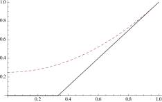
Figure 1. Separable states take zero values, while entangled states take positive values according to the concurrence $\mathcal{C}(\rho_{W})$ (straight line). The purity $\mathrm{Tr}(\rho_{W}\widetilde{\rho_{W}})=\mathrm{Tr}(\rho_{W}^{2})$ yields an entanglement monotone, which provides a fair approximation of the concurrence $\mathcal{C}(\rho_{W})$ for $x\rightarrow 1$.

4.2. A two-parameter subclass of entangled states

By recalling the Schmidt-decomposed family of pure states associated to the vector

$$\left|\alpha_{0}\right\rangle:=\cos(\alpha_{0})\begin{pmatrix}1\\ 0\end{pmatrix}\otimes\begin{pmatrix}1\\ 0\end{pmatrix}+\sin(\alpha_{0})\begin{pmatrix}0\\ 1\end{pmatrix}\otimes\begin{pmatrix}0\\ 1\end{pmatrix},$$ (4.23)

having been used in the previous work for the identification of pull-back tensor fields on Schmidt-equivalence classes [2], we may now consider a convex combination

$$\rho_{x,\alpha_{0}}:=x\left|\alpha_{0}\right\rangle\left\langle\alpha_{0}\right|+(1-x)\rho^{*},$$ (4.24)

with a maximal mixed state $\rho^{*}$. Such a convex combination contains the 1-parameter family of Werner states as special case for $\alpha_{0}=\pi/4$. Computing here, the purity-related invariant $f_{2}^{R}(\rho)\equiv\left\langle\theta^{\rho}_{R}\vphantom{\theta^{\rho}_{R}}\right.\left|\vphantom{\theta^{\rho}_{R}}\theta^{\rho}_{R}\right\rangle$ yields

$$f_{2}^{R}(\rho_{x,\alpha_{0}})=f_{2}^{R}(\rho_{Werner})=6\left(x^{2}+1\right).$$ (4.25)

Next we shall consider in addition, the non-linear realization, given by

$$f_{2}^{\tilde{R}}(\rho)=\left\langle\theta^{\rho}_{\tilde{R}}\vphantom{\theta^{\rho}_{\tilde{R}}}\right.\left|\vphantom{\theta^{\rho}_{\tilde{R}}}\theta^{\rho}_{\tilde{R}}\right\rangle\quad\mbox{ with }\tilde{R}(X_{j})=[R(X_{j})-\rho(R(X_{j}))\mathds{1}]\rho$$ (4.26)

to see what happens. Here we find

$$f_{2}^{\tilde{R}}(\rho_{x,\alpha_{0}})=2\cos\left(4\alpha_{0}\right)x^{4}+\frac{1}{2}\cos\left(8\alpha_{0}\right)x^{4}+\frac{3x^{4}}{2}$$

$$-2\cos\left(4\alpha_{0}\right)x^{3}-2x^{3}-2\cos\left(4\alpha_{0}\right)x^{2}+4x^{2}+6.$$ (4.27)

Hence, in contrast to the Hermitian representation $R$, the non-linear realization $\tilde{R}$ is able to captures the information on the additional parameter $\alpha_{0}$. Moreover it involves a $x$-dependence beyond quadratic order. This suggests to introduce a ‘non-linear’ extended version of the purity measure by

$$\mathcal{D}(\rho):=\frac{1}{8}f_{2}^{\tilde{R}}(\rho_{x,\alpha_{0}})-\frac{1}{2}.$$ (4.28)

This quantity shall now be compared with the concurrence $\mathcal{C}(\rho)$ by applying both functions on the considered two-parameter subclass of states $\rho_{x,\alpha_{0}}$. The concurrence $\mathcal{C}(\rho_{x,\alpha_{0}})$ yields here

$$\mbox{max}[-\frac{x^{2}}{8}+\frac{x}{4}+\frac{1}{2}\sqrt{-x^{2}\left(2\cos\left(4\alpha_{0}\right)x^{2}+(x-2)x-1\right)\sin^{2}\left(2\alpha_{0}\right)}-\frac{1}{8},0].$$ (4.29)

The latter function is plotted in figure 2, while the ‘non-linear’ extended version of the purity is given in figure 3.

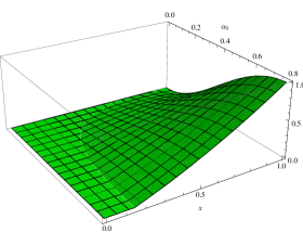
Figure 2. Separable states take zero values, while entangled states take positive values according to the concurrence $\mathcal{C}(\rho_{x,\alpha_{0}})$.

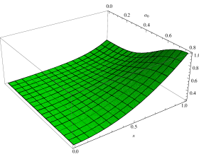
Figure 3. A possible approximation of the concurrence measure derived from an non-linear realization-dependent IOVT, giving rise to the invariant $\mathcal{D}(\rho_{x,\alpha_{0}})$.

In this regard we may compute the functional dependence between both functions by

$$d\mathcal{C}\wedge d\mathcal{D}=0:\Leftrightarrow\mbox{$\mathcal{C}$ and $\mathcal{D}$ are functional dependent,}$$ (4.30)

as it has been considered in [5]. The corresponding plot is given in figure 4, where a region of functional independence exists.

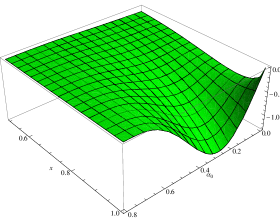
Figure 4. The functional dependence $d\mathcal{C}\wedge d\mathcal{D}$ between both functions is given for all parameter combinations with vanishing values.

5. Conclusions and Outlook

In this work we have approached the separability problem of entangled mixed states $\rho$ on finite-dimensional product Hilbert spaces by means of an evaluation on invariant operator-valued tensor fields (IOVTs)

$$\theta_{R}:=\bigg{(}\prod_{a=1}^{k}R(X_{i_{a}})\bigg{)}\bigotimes_{a=1}^{k}\theta^{i_{a}}$$ (5.1)

on the unitary group $SU(n)\times SU(n)$. By mapping the resulting invariant classical tensor fields

$$\quad\theta^{\rho}_{R}:=\rho\bigg{(}\prod_{a=1}^{k}R(X_{i_{a}})\bigg{)}\bigotimes_{a=1}^{k}\theta^{i_{a}}$$ (5.2)

in terms of Hermitian inner product contractions to real-valued polynomial functions

$$f_{k}^{R}(\rho):=\sum_{n}a_{n}\left\langle\theta^{\rho}_{R}\vphantom{\theta^{\rho}_{R}}\right.\left|\vphantom{\theta^{\rho}_{R}}\theta^{\rho}_{R}\right\rangle^{n},$$

the concept of $R$-classes of entanglement monotones candidates emerged in dependence of the choice of a realization $R$ of the underlying Lie algebra. Let us outline in detail the two possible main practical merits of this approach for future works.
First, in the case of pure states, we may deal with the idea of an algorithmic procedure to identify $SU(n)\times SU(n)$-invariant functions on Schmidt-equivalence classes (i.e. local-unitarily generated orbits) which crucially evades the computational effort of a singular value decomposition into Schmidt-coefficients. This idea might be illustrated by the fact that Schmidt-equivalence classes provide homogenous spaces [23, 24, 25], suggesting a local, rather than a global, approach to be sufficient for extracting the information on the entanglement of the state which belongs to the corresponding orbit. Invariant covariant tensor field constructions on $SU(n)\times SU(n)$, as discussed in part I.  in [2], relate to pull-back tensor fields from the ‘quotient’, i.e. from a Schmidt-equivalence class orbit and provide therefore clearly, the most natural tool for extracting this information.
Second, within the generalized case of mixed states, one may foresee the existence a ‘functorial’ correspondence between certain classes of separability criteria and $R$-classes of entanglement monotones candidates. To illustrate such a relation, we observe that we recover for the non-linear realization

$$\tilde{R}(X_{j})=R(X_{j})-\rho(R(X_{j}))\mathds{1},$$ (5.3)

and the associated covariance matrix-tensor field

$$\theta^{\rho}_{\tilde{R}}=(\rho(R(X_{j})R(X_{k}))-\rho(R(X_{j}))\rho(R(X_{k}))\theta^{j}\otimes\theta^{k},$$ (5.4)

a class of separability criteria having their origin in the so-called covariance matrix criterion [26]. While the corresponding ‘linear $R$-subclass’ of criteria in the Bloch-representation proposed by de Vicente [21], has been illustrated here in section 3.3, we find for $n=2$,

$$\frac{1}{8}\big{(}\left\langle L^{\rho}_{R}\vphantom{L^{\rho}_{R}}\right.\left|\vphantom{L^{\rho}_{R}}L^{\rho}_{R}\right\rangle+(-1)^{j}\left\langle\Omega^{\rho}_{R}\vphantom{\Omega^{\rho}_{R}}\right.\left|\vphantom{\Omega^{\rho}_{R}}\Omega^{\rho}_{R}\right\rangle\big{)}-\frac{1}{2}=\begin{cases}\mbox{Tr}(\rho^{2})&\text{ for }j=0\\ \mbox{Tr}(\rho\tilde{\rho})&\text{ for }j=1.\end{cases}$$ (5.5)

and therefore the purity $\mathrm{Tr}(\rho^{2})$, the linear entropy $1-\mathrm{Tr}(\rho^{2})$ and the concurrence related quantity

$$4\mathrm{Tr}(\rho\widetilde{\rho})=1-\sum_{j=1}^{3}m_{j}^{2}-\sum_{j=1}^{3}n_{j}^{2}+\sum_{j,k=1}^{3}C_{j,k}^{2},$$ (5.6)

to be in such a linear $R$-subclass according to our classification of entanglement monotone candidates. A generalization of (5.6) to higher dimensions may shed some light on the geometric origin of the sufficient separability criterion based on the Bloch-representation in Proposition 3.8. The latter reads for two qubits

$$\sqrt{\sum_{k=1}^{3}n_{j}^{2}}+\sqrt{\sum_{k=1}^{3}m_{k}^{2}}+\mathrm{Tr}(\sqrt{C^{\dagger}C})\leq 1$$ (5.7)

and clearly outlines a link to (5.6). The tensorial picture may therefore allow to face the open problem (as given in [26]) to relate the ‘non-linear $\tilde{R}$-class’ of covariance matrix separability criteria to quantitative statements. In what has been said here, this could now be approached by a $\tilde{R}$-class of entanglement monotone candidates in terms of associated polynomials

$$f_{2}^{\tilde{R}}(\rho)=\sum_{n}a_{n}\left\langle\theta^{\rho}_{\tilde{R}}\vphantom{\theta^{\rho}_{\tilde{R}}}\right.\left|\vphantom{\theta^{\rho}_{\tilde{R}}}\theta^{\rho}_{\tilde{R}}\right\rangle^{n}.$$ (5.8)

In particular, the ‘first order term’ $\left\langle\theta^{\rho}_{\tilde{R}}\vphantom{\theta^{\rho}_{\tilde{R}}}\right.\left|\vphantom{\theta^{\rho}_{\tilde{R}}}\theta^{\rho}_{\tilde{R}}\right\rangle$ indicated within the examples of a two-parameter family of entangled states in the previous section, a possible approximation to the concurrence measure.
The identification of non-linear structures of higher order being hidden in the description of quantum entanglement may turn out to be crucial to tackle the separability problem in both necessary and sufficient directions. This can be seen, already for the case of two qubits, by taking into account the relation between the Peres-Horodecki PPT-criterion [27, 28] and the role of so-called local filtering operations within the class of covariance matrix criteria [26].

The relation to the PPT-criterion

For this purposes, let us observe, that within the linear $R$-class, we are let to consider either sufficient or necessary criteria, where we found a strong indication that the anti-symmetric IOVT

$$\Omega:=[R(X_{j}),R(X_{k})]_{-}\theta^{j}\wedge\theta^{k}$$

associated with the coefficients

$$\Omega^{A}_{[jk]}(\rho)=\mathrm{Tr}(\rho^{A}[\sigma_{j},\sigma_{k}]_{-}),\qquad\Omega^{B}_{[jk]}(\rho)=\mathrm{Tr}(\rho^{B}[\sigma_{j-n^{2}},\sigma_{k-n^{2}}]_{-})$$ (5.9)

plays a fundamental role to measure ‘how far’ the necessary criterion (Theorem 3.9) is from being also a sufficient criterion (Theorem 3.10). Specifically for a qubit system, we may identify the imaginary ‘eigenvalues’ of $(\Omega^{A}_{[jk]}(\rho))$ and $(\Omega^{B}_{[jk]}(\rho))$ in dependence of the subsystem’s Bloch-representation coefficients $n_{j}$ and $m_{k}$ by

$$\pm i\sqrt{\sum_{k=1}^{3}n_{j}^{2}},\qquad\pm i\sqrt{\sum_{k=1}^{3}m_{k}^{2}}.$$ (5.10)

For generic entangled mixed states in $n=2$, having not maximal mixed subsystems as in the case of Werner states used in the previous section, the criterion in corollary 3.11 fails to be both sufficient and necessary. A way of making this criterion stronger is given by considering the complexification of the local special unitary transformations to $SL(2,\mathbb{C})\times SL(2,\mathbb{C})$. In particular, as it has been shown in [29], any state $\rho\in D(\mathbb{C}^{2}\otimes\mathbb{C}^{2})$ can be transformed via $SL(2,\mathbb{C})\times SL(2,\mathbb{C})$ into the so called standard form

$$\rho_{S}:=\frac{1}{4}(\sigma_{0}\otimes\sigma_{0}+d_{j}\sigma_{j}\otimes\sigma_{j})$$ (5.11)

with $(d_{1},d_{2},d_{3})\in\triangle_{2}\subset\mathbb{R}^{3},$ parametrizing points on a 3-dimensional convex subset given by a tetrahedron, i.e. a 2-simplex $\triangle_{2}$. By evaluating the resulting standard form (5.11) on a symmetric IOVT

$$L:=[R(X_{j}),R(X_{k})]_{+}\theta^{j}\odot\theta^{k}$$ (5.12)

associated as in the previous sections to a product representation $SU(2)\times SU(2)\rightarrow U(4)$, we find a matrix of coefficients decomposed in submatrices by

$$(L_{(jk)})(\rho_{S})=\left(\begin{array}[]{cc}A&C\\ C&B\end{array}\right),$$ (5.13)

with $A(\rho_{S})=B(\rho_{S})=\mathds{1}$ and

$$C(\rho_{S})=\left(\begin{array}[]{lll}d_{1}&0&0\\ 0&d_{2}&0\\ 0&0&d_{3}\end{array}\right).$$ (5.14)

By comparing with (4.7), it becomes evident that the class of Werner states are recovered here by the constraint

$$d_{1}=d_{3}=-d_{2}.$$ (5.15)

In contrast to the symmetric IOVT, the evaluation on an anti-symmetric IOVT $\Omega:=[R(X_{j}),R(X_{k})]_{-}\theta^{j}\wedge\theta^{k}$ will in general yield a maximal degenerate tensor field

$$(\Omega_{(jk)})(\rho_{S})=0.$$ (5.16)

Now one may observe the following. A partial transposition (PT) of the matrix representation of $\rho_{S}$ induces a transformation on $C(\rho_{S})$ given by a reflection on the second diagonal element

$$C(\rho_{S})=\left(\begin{array}[]{lll}d_{1}&0&0\\ 0&d_{2}&0\\ 0&0&d_{3}\end{array}\right)\mapsto C(\rho_{S}^{PT})=\left(\begin{array}[]{lll}d_{1}&0&0\\ 0&-d_{2}&0\\ 0&0&d_{3}\end{array}\right).$$ (5.17)

As it has been argued in [29], the intersection

$$\triangle_{2}\cap PT^{*}(\triangle_{2})\equiv\mathcal{S}$$ (5.18)

of the 2-simplex $\triangle_{2}$ with its PT-induced reflection $PT^{*}(\triangle_{2})$ is identical to the set $\mathcal{S}$ of separable states, which provides an octahedron, defined by the constraint

$$\sum_{j=1}^{3}|d_{j}|\leq 1.$$ (5.19)

The later condition turns out to be equivalent to

$$\|C(\rho_{S})\|_{KF}\leq 1,$$ (5.20)

and crucially, generalizes the separability criterion in corollary 3.11 for states with maximal mixed subsystems to generic states, whenever one makes use of a ‘local filtering’ operation $\rho\mapsto\rho_{S}$ induced by $SL(2,\mathbb{C})\times SL(2,\mathbb{C})\subset SL(4,\mathbb{C})$.
The latter group preserves the positive cone structure in $u^{*}(\mathbb{C}^{2}\otimes\mathbb{C}^{2})\cong u^{*}(\mathbb{C}^{4})$, which may allow to recover here as a consequence the Peres-Horodecki criterion [27, 28], which states that a state in $D(\mathbb{C}^{2}\otimes\mathbb{C}^{2})$ is separable iff its matrix representation remains positive under partial transposition.
In this regard it would be interesting to construct IOVTs, on the Lie group $\mathcal{G}\equiv SL(2,\mathbb{C})\times SL(2,\mathbb{C})$ to identify pull-back tensor fields from homogeneous space manifolds $\mathcal{G}/\mathcal{G}_{0}$. The latter may become identified in this regard with distinguished strata $D^{k}(\mathcal{H})\subset D(\mathcal{H})$ of mixed states $\rho$ with fixed rank $k$, whenever one considers the non-linear action

$$\rho\mapsto\frac{T\rho T^{\dagger}}{\mathrm{Tr}(T\rho T^{\dagger})},\quad T\in G=GL(\mathcal{H})$$ (5.21)

as shown in [30, 31]. By identifying the corresponding infinitesimal action of this non-linear action, in terms of vector fields resp. non-linear operators, one may build a corresponding IOVT, whose evaluation on a state with fixed rank $k$ may gives rise to a pull-back tensor from $D^{k}(\mathcal{H})$ to $\mathcal{G}=GL(\mathcal{H})$.
Such a construction could provide a tensor field which is invariant under the so called ‘local filtering operations’ associated to the subgroup

$$SL(2,\mathbb{C})\times SL(2,\mathbb{C})\subset GL(4,\mathbb{C}),$$ (5.22)

which transforms a given state $\rho$ to its standard form (5.11). Invariant tensor field on these orbits could pave the way to reduce the computational effort of a local filtering operation, in analogy to invariant tensor fields on Schmidt-equivalence classes, which reduce the computational effort of a Schmidt-decomposition. This issue shall be worked out in detail, both for two qubits, but also in higher dimensional composite systems in a forthcoming paper.

References

- [1] P. Aniello, G. Marmo, and G. F. Volkert. Classical tensors from quantum states. Int. J. Geom. Meth. Mod. Phys., 07:369–383, 2009.
- [2] P. Aniello, J. Clemente-Gallardo, G. Marmo, and G. F. Volkert. Classical Tensors and Quantum Entanglement I: Pure States. Int. J. Geom. Meth. Mod. Phys., 7:485, 2010.
- [3] A. M. Perelomov. Coherent states for arbitrary Lie group. Communications in Mathematical Physics, 26:222, 1972.
- [4] A. Ashtekar and T. A. Schilling. Geometrical Formulation of Quantum Mechanics. In A. Harvey, editor, On Einstein’s Path: Essays in honor of Engelbert Schucking, page 23, (1999).
- [5] J. Clemente-Gallardo and G. Marmo. Basics of Quantum Mechanics, Geometrization and Some Applications to Quantum Information. International Journal of Geometric Methods in Modern Physics, 5:989, 2008.
- [6] D. C. Brody and L. P. Hughston. Geometric quantum mechanics. Journal of Geometry and Physics, 38:19–53, April 2001.
- [7] J. F. Cariñena, J. Clemente-Gallardo, and G. Marmo. Geometrization of quantum mechanics. Theoretical and Mathematical Physics, 152:894–903, July 2007.
- [8] D. Chruscinski and G. Marmo. Remarks on the GNS Representation and the Geometry of Quantum States. Open Syst. Info. Dyn., 16:157–177, 2009.
- [9] A. Ibort, V. I. Man’ko, G. Marmo, A. Simoni, and F. Ventriglia. An introduction to the tomographic picture of quantum mechanics. Physica Scripta, 79(6):065013, June 2009.
- [10] P. Aniello. Star products: a group-theoretical point of view. Journal of Physics A Mathematical General, 42:5210, November 2009.
- [11] G. F. Volkert. Tensor fields on orbits of quantum states and applications. Dissertation, LMU München: Fakultät für Mathematik, Informatik und Statistik, Aug 2010.
- [12] S. Helgason. Differential geometry and symmetric spaces. Pure Appl. Math. Academic Press, New York, NY, 1962.
- [13] V. I. Arnold. Les methodes mathematiques de la Mecanique Classique. Editions Mir, Moscow, 1976.
- [14] I. Bengtsson. A Curious Geometrical Fact about Entanglement. In G. Adenier, A. Y. Khrennikov, P. Lahti, & V. I. Man’ko, editor, Quantum Theory: Reconsideration of Foundations, volume 962 of American Institute of Physics Conference Series, pages 34–38, (2007).
- [15] G. Vidal. Entanglement monotones. Journal of Modern Optics, 47:355–376, February 2000.
- [16] William K. Wootters. Entanglement of Formation of an Arbitrary State of Two Qubits. Phys. Rev. Lett., 80(10):2245–2248, Mar 1998.
- [17] V. Coffman, J. Kundu, and W. K. Wootters. Distributed entanglement. Phys. Rev. A, 61(5):052306, Apr 2000.
- [18] G. Jaeger, A. V. Sergienko, B. E. A. Saleh, and M. C. Teich. Entanglement, mixedness, and spin-flip symmetry in multiple-qubit systems. Phys. Rev. A, 68(2):022318, Aug 2003.
- [19] I. Bengtsson and K. Życzkowski. Geometry of Quantum States. Cambridge University Press, New York, 2006.
- [20] L. Gurvits. Classical deterministic complexity of Edmonds’ Problem and quantum entanglement. In STOC ’03: Proceedings of the thirty-fifth annual ACM symposium on Theory of computing, ACM, New York, pages 10–19, (2003).
- [21] J. I. De Vicente. Separability criteria based on the Bloch representation of density matrices. Quantum Inf. Comput., 7:624, 2007.
- [22] R. F. Werner. Quantum states with Einstein-Podolsky-Rosen correlations admitting a hidden-variable model. Phys. Rev. A, 40(8):4277–4281, Oct 1989.
- [23] Marek Kuś and Karol Życzkowski. Geometry of entangled states. Phys. Rev. A, 63(3):032307, Feb 2001.
- [24] M. M. Sinolecka, K. Życzkowski, and M. Kuś. Manifolds of Equal Entanglement for Composite Quantum Systems. Acta Physica Polonica B, 33:2081, August 2002.
- [25] P. Aniello and C. Lupo. On the relation between Schmidt coefficients and entanglement. Open Sys. Information Dyn., 16:127, 2009.
- [26] O. Gittsovich, O. Gühne, P. Hyllus, and J. Eisert. Unifying several separability conditions using the covariance matrix criterion. Phys. Rev. A, 78(5):052319, Nov 2008.
- [27] A. Peres. Separability criterion for density matrices. Phys. Rev. Lett., 77(8):1413–1415, Aug 1996.
- [28] M. Horodecki, P. Horodecki, and R. Horodecki. Separability of mixed states: necessary and sufficient conditions. Physics Letters A, 223:1–8, February 1996.
- [29] J. M. Leinaas, J. Myrheim, and E. Ovrum. Geometrical aspects of entanglement. Phys. Rev. A, 74(1):012313, Jul 2006.
- [30] J. Grabowski, M. Kuś, and G. Marmo. Symmetries, group actions, and entanglement. Open Sys. Information Dyn., 13:343–362, 2006.
- [31] J. Grabowski, M. Kuś, and G. Marmo. Geometry of quantum systems: density states and entanglement. Journal of Physics A Mathematical General, 38:10217–10244, December 2005.