Convergence of a renormalization group approach to dimer-dimer scattering

Abstract

We study the convergence of a functional renormalisation group technique by looking at the ratio between the fermion-fermion scattering length and the dimer-dimer scattering length for a system of nonrelativistic fermions. We find that in a systematic expansion in powers of the fields there is a rapid convergence of the result that agrees with know exact results.

I introduction

The atomic physics of ultra-cold Fermi gases is one of the places where we can make a detailed link few-particle and many-body physics. In fermionic systems we can trace the effect of an attractive force from the bound states or resonances in few-body systems to the pairing occurring in the many-body sector. At low energy and in cold gases this physics is governed by a single parameter, the central $S$-wave scattering length $a_{F}$, determining the scattering at threshold. We can also tune the value of this scattering length making use of recent advances using Feshbach resonances. For negative scattering length the gas is in the weak-coupling BCS state. For positive values of $a_{F}$ bound states of two fermions–“dimers”–form and these can lead to a Bose-Einstein condensate (BEC) Zwe . The size of dimers is determined by the fermion-fermion scattering length and their binding energy is of order $1/a_{F}^{2}$.

If we concentrate on the case of deeply-bound dimers, then for a sufficiently dilute and cold gas of dimers the main dynamical quantity characterising their interaction is now the dimer-dimer scattering length $a_{B}$, which is a induced by the fermionic scattering. The exact relation between dimer-dimer and fermion-fermion scattering lengths $a_{B}=0.6a_{F}$ was established in Ref. Shl by solving the Schr dinger equation for two composite bosons interacting with an attractive zero-range potential. Unfortunately, this method is difficult to extend to the many-body case. Therefore, it is useful to study the ratio $a_{B}/a_{F}$ in an approach which can be used both for few and many-body problems.

One such method is the functional or “exact” renormalisation group (ERG) for the one-particle irreducible effective action, which is the approach applied in this paper to calculate $a_{B}$. (For reviews, see Refs. BTW ; DMT ). This technique has been previously used to study a variety of physical systems, from systems of nonrelativistic fermions Kri ; Kri2 ; Diehl ; Bir ; DKS ; Flo ; Flo2 and bosons SandM to quark models JW and gauge theories LPG . It is based on the scale-dependent quantum effective action $\Gamma_{k}$, where the action at scale $k$ contains the effects of field fluctuations with momenta $q$ larger than $k$ only. In the limit $k\rightarrow 0^{+}$ all fluctuations are included and the full effective action is recovered. In practice the scale dependence is introduced by a set of $k$-dependent cutoff functions $R(q)$, which suppress the effect of modes with $q<k$ in the path integral for the action by giving them a large $k$ dependent mass. The minimal conditions satisfied by the functions $R(q)$ are then that they should vanish in the limit $k\rightarrow 0^{+}$ and scale like $k^{\alpha}$ with $\alpha>0$ when $k\rightarrow\infty$ .

With this prescription the average effective action at very large $k$ converges to the classical action of the theory—here nonrelativistic fermions with a local zero-range interaction. Since one can show that we get the effective action for the theory as $k\rightarrow 0^{+}$, the endpoint at $k=0$ of the exact solution of the functional RG equation should be independent of the choice of cutoff. However, in practice, truncations of the action inevitably lead to some cutoff dependence of the results. We can use this dependence as one possible measure of the quality of the truncation. With this tool, we shall analyse the convergence of a low-energy long-wavelength expansion as we increase the complexity of the many-body truncation in the effective action.

As discussed in great detail in the literature, e.g. Ref. (Wein2, , Chapter 16), the idea of the (quantum) effective action $\Gamma$ is to introduce an object that generalises the concept of the classical action of a field theory to include all quantum effects, but still depends on a set of classical external fields (the dual of the usual external sources in the partition function). The ground state is the minimum of the action, and we can generate all Green functions by appropriate derivatives of $\Gamma$. Apart from for very simple models, it is very hard to explicitly evaluate the full effective action, which is given by a complicated path integral. The ERG technique used here gives a scale-dependent mass-gap to the low-momentum modes in the path integral, so that their fluctuations are suppressed. The action then flows from the trivial case of all fluctuations suppressed (scale $k$ is infinite) to the full quantum effective action for zero scale. Since this approach in principle incorporates the full quantum dynamics of the underlying theory, it is called “exact”.

The flow of the effective action satisfies the functional differential equation BTW

$$\partial_{k}\Gamma=-\frac{i}{2}\,\operatorname{STr}\left[(\partial_{k}R)\,(\Gamma^{(2)}-R)^{-1}\right].$$ (1)

where $\Gamma^{(2)}$ is the second functional derivative with respect to the fields, and the cutoff functions in the mass-like term $R(k)$ drive the RG evolution. The operation $\operatorname{STr}$ denotes the supertrace Ma taken over energy-momentum variables and internal indices and is defined by

$$\operatorname{STr}\left(\begin{array}[]{cc}A_{BB}&A_{BF}\\ A_{FB}&A_{FF}\end{array}\right)=\operatorname{Tr}(A_{BB})-\operatorname{Tr}(A_{FF}).$$ (2)

The evolution equation for the average effective action thus has a one-loop structure, but contains a fully dressed, scale-dependent propagator $(\Gamma^{(2)}-R)^{-1}$. Thus, despite its apparently simple form, Eq. (1) is actually a complex functional differential equation. In the absence of general methods to numerically solve such equations we must resort to approximations. One common approach is to parametrise the effective action with a small number of terms, which turns the evolution equation into a system of coupled ordinary differential equations for the numerical coefficient of each term. These equations can then be solved numerically. Here we study possible truncations for fermionic few-body systems, and our choice of ansatz for the action is motivated by both ERG studies of many-body systems Kri ; Diehl and effective field theories (EFTs) for few-fermion systems EFT . The technique we use is similar to the one used in Ref. Bir and Ref. Kri2 . The parametrisation of the effective action is given by a local expansion in fundamental and induced fields, with a simple gradient expansion for non-local terms.

There are a number of questions about the approximations made in writing down the action. We shall try and answer two of these in this paper: Firstly, does the low-energy truncation, where we expand to first order in energy and to first order in field-gradient squared converge? Secondly, are these results independent of the choice of cut-off function? These two questions are not independent: If we have a converged truncation of the effective action, we must have independence of the cut-off function. Reversing this, we can hope that the dependence on the cut-off can be used as one of the signals of convergence.

The renormalisation functions $R(q)$ is not completely arbitrary: as the cutoff scale tends to infinity, we demand that the action be purely fermionic, containing a contact two-body interaction without derivatives. Such interactions are of interest also for interacting nucleons EFT . In both these cases, it is convenient to add an auxiliary composite boson field (which is really the dimer field) to the problem by making a Hubbard-Stratonovich transformation. This then replaces the two-body interaction by a Yukawa-type coupling between the fermions and the auxiliary boson. At the extreme end of the scale, the boson is not dynamic (there is no energy or momentum dependence of this field in the action), but a kinetic term for the boson is generated in the RG evolution.

II Building blocks

We define the low-energy effective action following previous work (see Kri ; Diehl ; Bir ; Kri2 ; SandM ) as an expansion in the fermion fields $\psi$–a two-component spinor field, where the index denotes fermion spin– and the scalar dimer boson field $\phi$ obtained from bosonising the bilinear fermion field $\psi^{{\rm T}}(x)\sigma_{2}\psi(x)$

$$\Gamma[\psi,\psi^{\dagger},\phi,\phi^{\dagger},k]$$

$$=\int d^{4}x\,\Biggl{[}\int d^{4}x^{\prime}\,\phi^{\dagger}(x)\Pi(x,x^{\prime};k)\phi(x^{\prime})$$

$$\quad+\psi^{\dagger}(x)\left(i\partial_{t}+\frac{1}{2M}\,\nabla^{2}\right)\psi(x)$$

$$\quad-\frac{i}{2}\,g\biggl{(}\psi^{{\rm T}}(x)\sigma_{2}\psi(x)\phi^{\dagger}(x)-\psi^{\dagger}(x)\sigma_{2}\psi^{\dagger{\rm T}}(x)\phi(x)\biggr{)}$$

$$\quad-\frac{1}{2}\,u_{2}\,\Bigl{(}\phi^{\dagger}(x)\phi(x)\Bigr{)}^{2}$$

$$\quad-\lambda\,\phi^{\dagger}(x)\phi(x)\psi^{\dagger}(x)\psi(x)$$

$$\quad-\frac{i}{4}\,g^{\prime}\Bigl{(}\phi^{\dagger}(x)\phi(x)\Bigr{)}$$

$$\qquad\biggl{(}\psi^{{\rm T}}(x)\sigma_{2}\psi(x)\phi^{\dagger}(x)-\psi^{\dagger}(x)\sigma_{2}\psi^{\dagger{\rm T}}(x)\phi(x)\biggr{)}$$

$$\quad-\frac{1}{4}\,\nu\,\Bigl{(}\phi^{\dagger}(x)\phi(x)\Bigr{)}\psi^{\dagger}(x)\sigma_{2}\psi^{\dagger{\rm T}}(x)\psi^{{\rm T}}(x)\sigma_{2}\psi(x)\Biggr{]}.$$ (3)

In contrast with the many-body case, in the few-body sector there is no wavefunction and mass renormalisation of the fermion field. The quantity $\Pi(x,x^{\prime},k)$ is the scale-dependent boson self-energy and $u_{2}$ parametrises the boson-boson interaction which is generated by the evolution. The latter is equivalent to a four-body interaction in terms of the underlying fermions. The term proportional to $\lambda$ describes the fermion-dimer scattering (three body in the fermions). The final two terms are four-body again: the term proportional to $g^{\prime}$ describes the scattering of two dimers, where one dimer breaks up into two fermions, and finally the $\nu$ term describes the scattering of two fermions from a dimer, without changing character. We have not included the local two-fermion interaction, which has zero coupling constant due to our choice of starting model at large (infinite scale), where only $g$ is nonzero.

The evolution of the boson self-energy is given by

$$\partial_{k}\Pi(x,x^{\prime},k)=\frac{\delta^{2}}{\delta\phi(x^{\prime})\delta\phi^{\dagger}(x)}\,\partial_{k}\Gamma|_{\phi=0},$$ (4)

although from now on we shall express all evolution in momentum space. Note that only fermion loops contribute to the evolution of the boson self-energy in vacuum.

Using a gradient expansion of the action, we can define boson wave-function and mass renormalisation factors by

$$Z_{\phi}(k)=\frac{\partial}{\partial P_{0}}\,\Pi(P_{0},\boldsymbol{P},k)\Biggr{|}_{P_{0}=\mathcal{E}_{D},\boldsymbol{P}=0},$$ (5)

and

$$\frac{1}{4M}\,Z_{m}(k)=-\frac{\partial}{\partial P^{2}}\,\Pi(P_{0},\boldsymbol{P},k)\Biggr{|}_{P_{0}=\mathcal{E}_{D},\boldsymbol{P}=0},$$ (6)

where $\mathcal{E}_{D}=-1/(Ma_{F}^{2})$ denotes the bound-state energy of a pair of fermions. It is relatively straightforward to show that $Z_{m}(0)=Z_{\phi}(0)$, independent of the cut-off function. There are very few cut-off functions that preserve Galilean invariance to quadratic order in momenta, but one favourite sharp cut-off Litim

$$R_{F}({\boldsymbol{q}},k)=\frac{k^{2}-q^{2}}{2M}\,\theta(k-q),$$ (7)

can be shown to preserve the identity $Z_{\phi}(k)=Z_{m}(k)$. Such sharp cut-off functions are difficult to apply in medium, since the evolution of $Z_{m}$ will contain ambiguous terms containing $\delta$ functions and their derivatives arising from the first and second derivative of the cut-off function. Such difficulties can be bypassed here since $\Pi$ can be evaluated directly. We first impose the boundary condition that the scattering amplitude in the physical limit $k\rightarrow 0$ reproduces the fermion-fermion scattering length,

$$\frac{1}{T(p)}=\frac{1}{g^{2}}\,\Pi(P_{0},P,0)=\frac{M}{4\pi a_{F}}\,.$$ (8)

Here $P_{0}\ (P)$ denotes the total energy (momentum) flowing through the system and $p=\sqrt{2MP_{0}-P^{2}/2}$ is the relative momentum of the two fermions. Integrating the resulting ERG equation gives Bir

$$\Pi(P_{0},P,k) = \frac{g^{2}M}{4\pi^{2}}\biggl{[}-\frac{4}{3}\,k+\frac{\pi}{a_{F}}+\frac{16}{3k}\left(MP_{0}-\frac{P^{2}}{2}\right)$$ (9)

$$\qquad\qquad-\frac{P^{3}}{24k^{2}}+...\biggr{]}.$$

This shows that Galilean invariance is preserved only to lowest order.

The complexity of sharp cut-off functions in medium implies that it is of interest to study smooth cut-offs, where both $Z$’s must now be calculated independently. A suitable set of smooth functions can be parametrised as

$$R_{F}({\boldsymbol{q}},k) =\frac{k^{2}}{2M}\,\theta_{\sigma}(q,k),$$

$$\theta_{\sigma}(q,k) =\frac{\operatorname{erf}\left((-q/k+1)/\sigma\right)+\operatorname{erf}\left((q/k+1)/\sigma\right)}{2\operatorname{erf}(1/\sigma)}.$$ (10)

II.1 Mean-field

In vacuum, it is easy to show that

$$Z_{\phi}(k) =\frac{g^{2}}{4}\int\frac{d^{3}{\boldsymbol{q}}}{(2\pi)^{3}}\,\frac{1}{\left(E_{FR}(\boldsymbol{q},k)-\mathcal{E}_{D}/2\right)^{2}},$$

$$Z_{m}(k) =\frac{g^{2}}{6}\int\frac{d^{3}{\boldsymbol{q}}}{(2\pi)^{3}}\,\frac{1}{6q\left(E_{FR}(\boldsymbol{q},k)-\mathcal{E}_{D}/2\right)^{2}}$$

$$\qquad\times\left(2\partial_{q}E_{FR}(\boldsymbol{q},k)+q\partial_{qq}E_{FR}(\boldsymbol{q},k)\right).$$

Thus

$$Z_{\phi}(0)=Z_{m}(0)=\frac{g^{2}a_{F}}{8\pi}.$$

The evolution of the boson-boson scattering amplitude follows from

$$-\frac{2}{(2\pi)^{4}}\partial_{k}u_{2}(\mathcal{E}_{D},k)=\frac{\delta^{4}}{\delta\phi^{2}(\mathcal{E}_{D},0)\delta\phi^{\dagger 2}(\mathcal{E}_{D},0)}\,\partial_{k}\Gamma|_{\phi=0}.$$ (11)

The driving term of this equation can be separated into fermionic and bosonic contributions containing $\partial_{k}R_{F}$ and $\partial_{k}R_{B}$, respectively. We first look at the “mean-field” result, where bosonic contributions are neglected. The evolution of $u_{2}$ is then given by

$$\partial_{k}u_{2}=-\frac{3g^{4}}{4}\int\frac{d^{3}{\boldsymbol{q}}}{(2\pi)^{3}}\,\frac{\partial_{k}R_{F}}{\left[(E_{FR}(\boldsymbol{q},k)-\mathcal{E}_{D}/2\right)]^{4}},$$ (12)

where

$$E_{FR}(\boldsymbol{q},k)=\frac{1}{2M}\,q^{2}+R_{F}(q,k).$$ (13)

Equation (12) is integrable, and we find with $u_{2}(\infty)=0$ that

$$u_{2}(k) =\frac{3g^{4}}{16}\int\frac{d^{3}{\boldsymbol{q}}}{(2\pi)^{3}}\,\frac{1}{\left[(E_{FR}(\boldsymbol{q},k)-\mathcal{E}_{D}/2\right)]^{3}},$$ (14)

$$u_{2}(0) =\frac{1}{16\pi}\,M^{3}g^{4}a_{F}^{3}.$$ (15)

The scattering amplitude at threshold is

$$T_{BB}=\frac{8\pi}{2M}\,a_{B}=\frac{2u_{2}(0)}{Z_{\phi}^{2}}=\frac{8\pi a_{F}}{M},$$ (16)

giving the well-known mean-field result $a_{B}=2a_{F}$ Ha which is far from the exact value $a_{B}=0.6a_{F}$ Shl . This implies that beyond-mean-field effects such as dimer-dimer rescattering must be considered.

II.2 Boson and mixed loops

To include such effects we must take into account the loops containing boson propagators. After some algebra, we find the driving term

$$\partial_{k}u_{2}|_{B}=\frac{u_{2}^{2}(k)}{2Z_{\phi}(k)}\int\frac{d^{3}{\boldsymbol{q}}}{(2\pi)^{3}}\,\frac{\partial_{k}R_{B}}{\left[E_{BR}(\boldsymbol{q},k)-\mathcal{E}_{D}\right]^{2}},$$ (17)

where

$$E_{BR}(\boldsymbol{q},k)=\frac{Z_{m}(k)}{4M}\,q^{2}+u_{1}(k)+R_{B}(q,k)$$ (18)

and

$$u_{1}(k)=-\Pi(\mathcal{E}_{D},0,k).$$ (19)

In the case of a sharp cutoff, we choose the bosonic cutoff function to be as close as possible in form to the fermionic one,

$$R_{B}(\boldsymbol{q},k)=Z_{m}(k)\frac{(c_{B}k)^{2}-q^{2}}{4M}\,\theta(c_{B}k-q),$$ (20)

apart from the addition of a parameter $c_{B}$, which sets the relative scale of the fermionic and bosonic regulators, and a factor of $Z_{m}$. The latter has the important advantage of leading to a consistent scaling behaviour, so that all contributions to a single evolution equation decay with the same power of $k$ for large $k$. Moreover it also gives $a_{F}$-scaling, where all terms in a single equation have the same dependence on $a_{F}$. Neither of these two conditions is actually required, and we shall show below that removing such restrictions may give us access to interesting information.

It has been shown for bosonic systems SandM , and it also shown in detail in Fig. 2 below, that the simple two-body truncation is insufficient. The complete set of contact interactions in the four-body sector includes not just the dimer-dimer term $u_{2}$, but also terms where the dimer is broken into two fermions, Eq.  (3). The evolution equation for any of the couplings is described by an expansion about the energy of the bound state pole for bosons, and half that energy for fermions, e.g.,

$$\partial_{k}\lambda=-\frac{i}{2}\,\frac{\delta^{4}\operatorname{STr}\left[\partial_{k}R(\Gamma^{(2)}-R)^{-1}\right]}{\delta\phi^{\dagger}\!(\mathcal{E}_{D},0)\delta\phi(\mathcal{E}_{D},0)\delta\psi^{\dagger}\!(\mathcal{E}_{D}/2,0)\delta\psi(\mathcal{E}_{D}/2,0)}.$$ (21)

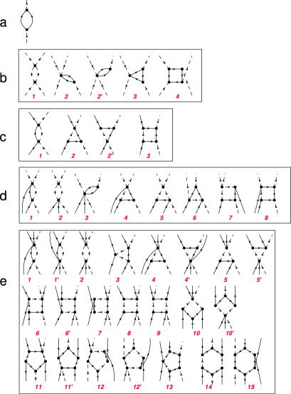
Figure 1: [Colour online] The skeletons of the diagrams that contribute to the evolution of the couplings. Dashed lines represent bosons, solid lines fermions. The dots represent the interaction vertices. In a) we show the diagrams for the evolution of $u_{1}$, $Z_{m}$ and $Z_{\phi}$ in b) for $u_{2}$, c) for $\lambda$, d) for $g^{\prime}$ and e) for $\nu$.

The technique to evaluate such contributions can most compactly be written as a combination of a diagrammatic and algebraic approach. We first evaluate the skeleton diagrams that contribute to a given vertex. There are three distinct contributions to the running of $\lambda$, coming from ladder, triangle and box diagrams, as shown in Fig. 1. For the other couplings, we have a large number of diagrams that can contribute. The most difficult calculation is for $g^{\prime}$, where we have loops with up to six internal lines. Each diagram involves a single integration over an internal four momentum. Since our cut-off function is only momentum-dependent, i..e., is independent of the energy variable, we can perform the energy integration by a contour integration, enumerating the poles by solving linear algebraic equations. The insertion of the $k$ derivative of the cut-off function on each leg can then be achieved afterwards, by a functional derivative of the resulting integrals with respect to the cut-off function.

The resulting equations can be written in a compact form as,

$$\partial_{\kappa}u_{2}(\kappa) =\frac{1}{2}I_{3,0,0}-\frac{1}{Z_{\phi}}I_{0,1,0}u_{2}(\kappa)^{2}+2I_{2,0,0}\lambda(\kappa)-2I_{1,0,0}g^{\prime}(\kappa),$$

$$\partial_{\kappa}\lambda(\kappa) =-\frac{1}{2}I_{2,0,1}-2I_{1,0,1}\lambda(\kappa)-2I_{0,0,1}\lambda(\kappa)^{2}$$

$$\partial_{\kappa}g^{\prime}(\kappa) =-2I_{1,0,1}g^{\prime}(\kappa)-4I_{0,0,1}g^{\prime}(\kappa)\lambda(\kappa)+\frac{-1}{Z_{\phi}}I_{0,1,0}g^{\prime}(\kappa)u_{2}(\kappa)$$

$$\quad+2I_{1,1,1}u_{2}(\kappa)+2I_{2,0,1}\lambda(\kappa)+4I_{1,0,1}u_{2}(\kappa)\lambda(\kappa)+4I_{1,0,1}\lambda(\kappa)^{2}-2I_{1,0,0}\nu(\kappa)$$

$$-\partial_{\kappa}\nu(\kappa) =-\left(\frac{1}{2}I_{3,1,1,}+\frac{3}{2}Z_{\phi}I_{2,1,2}\right)-4I_{1,0,1}\nu(\kappa)-8I_{0,0,1}\nu(\kappa)\lambda(\kappa)$$

$$\quad-(I_{2,1,1}+7Z_{\phi}I_{1,1,2})\lambda(\kappa)+2(I_{1,1,1}-5Z_{\phi}I_{0,1,2})\lambda(\kappa)^{2}+4I_{0,0,2}\lambda(\kappa)^{3}$$

$$\quad+2I_{1,1,1}g^{\prime}(\kappa)-\frac{1}{2Z_{\phi}}I_{0,1,0}g^{\prime}(\kappa)^{2}+4I_{0,1,1}g^{\prime}(\kappa)\lambda(\kappa),$$

with the basic integrals

$$I_{n_{1}n_{2}n_{3}} =\frac{1}{2}\int_{0}^{\infty}dq^{\prime}\left[\partial_{k}R_{F}(q^{\prime})\frac{\delta}{\delta R_{F}(q^{\prime})}+\partial_{k}R_{B}(q^{\prime})\frac{\delta}{\delta R_{B}(q^{\prime})}\right]_{Z_{\phi}}$$

$$\qquad\frac{1}{(2\pi)^{3}}\int\frac{d^{3}q}{E_{\text{FR}}(q,k)^{n_{1}}E_{\text{BR}}(q,k)^{n_{2}}(E_{\text{BR}}(q,k)+Z_{\phi}E_{\text{FR}}(q,k))^{n_{3}}}.$$ (22)

III Results

III.1 Full evolution

In theory we should start integration of the evolution equations at infinity–in practice the results are numerically independent of the starting scale provided this is chosen to be at least $ka_{F}\simeq 100$. For $k\gg 1/a_{F}$ the system is in the universal “scaling regime”, and a stable fixed point, see below, governs the evolution until $k$ becomes comparable with $1/a_{F}$.

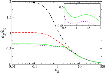
Figure 2: [Colour online] Ratio of dimer-dimer to fermion-fermion scattering lengths as a function of the relative scale parameter $c_{B}$. The black (dash-dotted) curve shows results for the minimal action; the red (dashed) curve shows the effect of adding the local three-body term; The green (solid) curve displays the full local four-body calculation, and is enlarged in the inset. The purple (dotted) line shows the effect of using a smooth cut-off ($\sigma=0.5$) on the full results.

In this scaling regime, we can determine the behaviour most easily in terms of dimensionless “scaling variable” $\kappa=ka_{F}$ by defining the four dimensionless functions $c_{i}(\kappa)$

$$u_{2}(\kappa) \to g^{4}M^{3}a_{F}^{3}\kappa^{-3}c_{0}(\kappa),$$

$$\lambda(\kappa) \to g^{2}Ma_{F}^{2}\kappa^{-2}c_{1}(\kappa),$$

$$g^{\prime}(\kappa) \to g^{3}M^{2}a_{F}^{4}\kappa^{-4}c_{2}(\kappa),$$

$$\nu(\kappa) \to g^{2}Ma_{F}^{5}\kappa^{-5}c_{3}(\kappa).$$ (23)

The functions $c_{i}$ satisfy a set of dimensionless differential equations. For each level of truncation of the effective action we can determine the resulting nontrivial fixed points, and the evolution close to these points, as given by the anomalous dimensions $\eta_{j}$,

$$c_{i}(\kappa)=c_{i}^{\text{fp}}+\sum_{j}a_{ij}\kappa^{\eta_{j}}.$$

For each truncation considered here we find only one stable fixed point, see Table 1. There we give the value for fixed point and anomalous dimensions for the sharp cut-off (7) with the parameter $c_{B}=1$ in the bosonic cut-off (20). These results are somewhat dependent on $c_{B}$, as expected, and are also not totally cut-off independent, but seem to be reasonably stable under perturbations.

Table 1: The coefficients and the eigenvalues of the stable fixed point for various level of truncation

truncation	fixed point	anomalous dimensions
$u_{2}$	$c_{0}=0.0656565$	$3.1728$
$u_{2},\lambda$	$c_{0}=0.037878,c_{1}=-0.322441$	$3.09969,3.10355$
$u_{2},\lambda,g^{\prime},\nu$	$\qquad c_{0}=0.0356522,c_{1}=-0.322441,\qquad$	$6.10943,5.15046,4.19149,3.10355$
	$c_{2}=0.102042,c_{3}=-10.488$

The dimension for $\lambda$,

$$\eta_{\lambda}=\frac{2}{5}\sqrt{\frac{301}{3}}\approx 3.10355$$ (24)

should be compared to the exact result $4.32244$, found by Griesshammer and others Grie ; Bir06 ; WeCa . The lowest anomalous dimension for the four-fermion sector, $4.19149$, should be compared with the value $5.0184$ obtained numerically by Stecher and Greene StG (see also Ref. ABF ).

If we start the evolution from the stable fixed point, we can then carefully trace this back to finite $k$. The behaviour of $a_{B}/a_{F}$ as a function of $c_{B}$ for both a sharp and a smooth cut-off with $\sigma=0.5$, Eqs. (7) and (10), is presented in Fig. 2. As we increase the complexity of the truncation, we see a rapid convergence: the inclusion of $\lambda$ reduces the size of $a_{B}$ by a factor of about 2 (for small $c_{B}$), and adding the remaining terms in the action pushes the result down even further to agree with the Schr dinger equation results; in that case we also see a very weak dependence on $c_{B}$ in the region around 1.

Note that in all cases the dominant contributions to $a_{B}/a_{F}$ for large $c_{B}$ come from the boson-loop terms in the equation for $u_{2}$. Since these do not depend on the three-body coupling $\lambda$, the curves approach each other. Moreover, this limit corresponds to integrating out the fermions first, which generates a non-zero value for $u_{2}$ at the start of the bosonic integration. In the limit $c_{B}\rightarrow\infty$, this coupling is driven to the trivial fixed point of the RG equations, $u_{2}=0$, since we have no terms to cancel the linearly divergent boson-boson loop diagram and the diagrams with three-body and four-body couplings are all too weak to alter this behaviour.

On the other hand, the main contributions for small $c_{B}$ come not only from the fermion loops, but also from mixed fermion-boson loops, which appear in the equations for the many-body couplings. In particular, the mixed boson-fermion loop diagrams containing the fermionic cut-off contribute to the evolution of $\lambda$, $\nu$ and $g^{\prime}$, even when the bosonic degrees of freedom have been integrated out. As a result, inclusion of the three-body term $\lambda$ already leads to a significant deviation from the mean-field result, $a_{B}/a_{F}=2$, that persists in the limit $c_{B}\rightarrow 0$. With $g^{\prime}$ and $\nu$ included we see convergence close to the exact result, even when $c_{B}=0$. We seem to have approximate convergence for a range of values of $c_{B}$, probably best near $c_{B}=1$, but we can probably use any $c_{B}\leq 1.5$. The strange results obtained for very large values of $c_{B}$ should not be taken too seriously, since they are based on an incorrect approach: we make the induced bosonic degrees of freedom dominate in the early stages of evolution (large $k$). The other extreme, albeit naively equally incorrect, actually seems to produce sensible results. This corresponds to freezing the renormalisation of the bosonic degrees of freedom, while still allowing an evolution of the coupling constants driven by the evolution of the fundamental fermionic fields, suggesting that this may be a sensible and simplifying approach. This may have important practical consequences for calculating in the many-body system: If we can integrate out the bosons at every stage, and only let the fermions evolve, the calculations become much simpler.

Arguments based on “optimisation” of the cut-off function, see Ref. Pawlowski , indicate that one should choose the cut-off to try to maximise the rate of convergence for our expansion of the action. In this case there is a stationary point for $c_{B}$ close to 1, which agrees with the natural assumption that $c_{B}=1$, where bosons and fermions are renormalised at the same rate is the optimal choice.

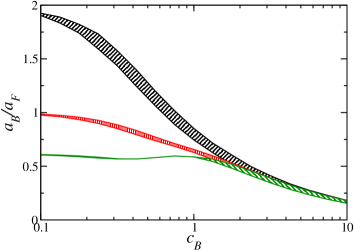
Figure 3: [Colour online] Ratio of dimer-dimer to fermion-fermion scattering lengths as a function of the relative scale parameter $c_{B}$. The black (right-slanted hash) curve shows results for the minimal action; the red (vertical hash) curve shows the effect of adding the local three-body term; The green (left-leaning hash) curve displays the full local four-body calculation. The width of each curve denotes the sensitivity of the result to changes in $a_{F}$ at $a_{F}=gM/\hbar^{2}$

To provide a further check of convergence, it pays to use a different form for the boson regulator, and purposefully violate both the uniform $a_{F}$-dependence and the uniform scaling for large $k$. If we have convergence, the results should remain independent of the cut-off, and thus also independent of $a_{F}$ and the shape of the cut-off function.. The simplest form we can choose uses the smooth cut-off function (10), where we renormalise the bosons as (note the absence of $Z_{m}$)

$$R_{B}=\frac{(kc_{B})^{2}}{2m_{D}}\theta_{\sigma}(q,kc_{B}).$$

With this choice we expect the ratio $a_{B}/a_{F}$ to be a function of $a_{F}$; we have first performed calculations at $a_{F}=1$, and looked at the sensitivity to changes in $a_{F}$. In Fig. 3 we see a strong dependence on $a_{F}$ for any value of $c_{B}\neq 0$ for the two-body truncation, a weaker dependence for the three-body case, and a very weak dependence for the four-body case, as long as we consider $c_{B}<1$. For large $c_{B}\geq 2$, where we let the bosons dominate, we have universally poor result whatever the truncation, in agreement with the discussion above.

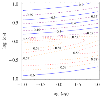
Figure 4: [Colour online] Ratio of dimer-dimer to fermion-fermion scattering lengths as a function of the relative scale parameter $c_{B}$, and the logarithm of the scattering length $a_{F}$ (divided by $gM/\hbar^{2}$). Notice the insensitivity to $a_{F}$ for $c_{B}<1$, a clear indication of convergence.

The convergence for the full four-body truncation can be seen even more clearly in Fig. 4, where we show a contour plot of the ratio of dimer-dimer and fermion-fermion scattering lengths as a function of $a_{F}$ and $c_{B}$. We note the excellent convergence in a large region of the parameter space, with allows a conservative estimate $a_{B}/a_{F}=0.58\pm 0.02$, in excellent agreement with the exact result.

IV Discussion

We have gathered considerable evidence for the convergence of a gradient expansion of the quantum effective action for a system of a few dilute fermions interacting through a pairwise attractive force. The resulting dimers, fermion-fermion bound states, scatter in the way predicted by exact calculations, if we expand the polarisation to second order in momenta, and include all the local four-body terms in the fermion and dimer fields.

Of course the expansion is only complete in terms of the number of fields that enter the action: we have neglected non-locality of all but the simplest terms, and have only included time derivatives to match the momentum dependence. In principle, we can add any momentum-dependence to any terms without problems; it is much more difficult to add energy dependent terms; with a momentum-dependent cut-off we are limited to first order terms only. Fortunately, it appears that we do not need such complications! As long as we study low-energy physics, which is exactly the situation here and in the many-body situation, that is not too surprising.

What does come as a surprise is that we seem to be able to fix the bosonic fields, and have an RG flow driven by the evolution of the fermionic fields only, while still obtaining good results. This is probably due to the fact that the evolution of the induced dimer degrees of freedom can be thought of as driven from the basic fermionic degrees of freedom through the coupling constants. This requires confirmation for finite density many-body systems.

- (1) M. Greiner, C. A. Regal and D. S. Jin, Nature 426, 537 (2003); S. Jochim, et al., Science 302, 2101 (2003); M. W. Zwierlein, et al., Phys. Rev. Lett. 91, 250401 (2003).
- (2) D. S. Petrov, C. Salomon and G. V. Shlyapnikov, Phys. Rev. Lett. 93, 090404 (2004).
- (3) J. Berges, N. Tetradis and C. Wetterich, Phys. Rept. 363, 223 (2002).
- (4) B. Delamotte, D. Mouhanna and M. Tissier, Phys. Rev. B 69, 134413 (2004).
- (5) M. C. Birse, B. Krippa, J. A. McGovern and N. R. Walet, Phys. Lett. B 605, 287 (2005).
- (6) B. Krippa, N. R. Walet, and M. C. Birse, Phys. Rev. A 81, 043628 (2010)
- (7) S. Diehl, H. Gies, J. M. Pawlowski and C. Wetterich, Phys. Rev. A 76, 021602(R) (2007); S. Diehl, H. Gies, J. M. Pawlowski and C. Wetterich, Phys. Rev. A 76, 053627 (2007).
- (8) M. C. Birse, Phys. Rev. C 77, 047001 (2008).
- (9) S. Diehl, H. C. Krahl, and M. Scherer, Phys. Rev. C 78, 034001 (2008).
- (10) S. Floerchinger, R. Schmidt, S. Moroz and C. Wetterich, Phys. Rev. A 79, 013603 (2009).
- (11) S. Floerchinger, M. M. Scherer and C. Wetterich, arXiv:0912.4050
- (12) R. Schmidt and S. Moroz, Phys. Rev. A81, 052709 (2010)
- (13) D.-U. Jungnickel and C. Wetterich, Phys. Rev. D53, 5142 (1996).
- (14) D. F. Litim and J. M. Pawlowski, Phys. Rev. D 66, 025030 (2002); H. Gies, Phys. Rev. D 66, 025006 (2002).
- (15) S. Weinberg, The quantum theory of fields, Vol 2 (Cambridge UP, Cambridge, 1996)
- (16) S. P. Martin, “A supersymmetry primer”, arXiv:hep-ph/9709356.
- (17) P. F. Bedaque and U. van Kolck, Ann. Rev. Nucl. Part. Sci. 52, 339 (2002).
- (18) S. Moroz, S. Floerchinger, R. Schmidt, C. Wetterich, Phys. Rev. A79, 042705 (2009).
- (19) D. F. Litim, Phys. Lett B 486, 92 (2000).
- (20) H. Griesshammer, Nucl. Phys. A 710, 110 (2005).
- (21) M. C. Birse, J. Phys. A: Math. Gen. 39, 249 (2006).
- (22) F. Werner and Y. Castin, Phys. Rev. Lett. 97, 150401 (2006)
- (23) J. von Stecker and C. H. Greene, Phys. Rev. A80, 022504 (2009).
- (24) Y. Alhassid, G. F. Bertsch and I. Fang, Phys. rev. Lett. 100, 230401 (2008)
- (25) R. Haussmann, Z. Phys. B 91, 291 (1993).
- (26) J. M. Pawlowski, Ann. Phys. 322, 2831 (2007).