An alternative to the plasma emission model: Particle-In-Cell, self-consistent electromagnetic wave emission simulations of solar type III radio bursts

Abstract

High-resolution (sub-Debye length grid size and 10000 particle species per cell), 1.5D Particle-in-Cell, relativistic, fully electromagnetic simulations are used to model electromagnetic wave emission generation in the context of solar type III radio bursts. The model studies generation of electromagnetic waves by a super-thermal, hot beam of electrons injected into a plasma thread that contains uniform longitudinal magnetic field and a parabolic density gradient. In effect, a single magnetic line connecting Sun to earth is considered, for which five cases are studied. (i) We find that the physical system without a beam is stable and only low amplitude level electromagnetic drift waves (noise) are excited. (ii) The beam injection direction is controlled by setting either longitudinal or oblique electron initial drift speed, i.e. by setting the beam pitch angle (the angle between the beam velocity vector and the direction of background magnetic field). In the case of zero pitch angle i.e. when $\vec{v}_{b}\cdot\vec{E}_{\perp}=0$, the beam excites only electrostatic, standing waves, oscillating at local plasma frequency, in the beam injection spatial location, and only low level electromagnetic drift wave noise is also generated. (iii) In the case of oblique beam pitch angles, i.e. when $\vec{v}_{b}\cdot\vec{E}_{\perp}\not=0$, again electrostatic waves with same properties are excited. However, now the beam also generates the electromagnetic waves with the properties commensurate to type III radio bursts. The latter is evidenced by the wavelet analysis of transverse electric field component, which shows that as the beam moves to the regions of lower density and hence lower plasma frequency, frequency of the electromagnetic waves drops accordingly. (iv) When the density gradient is removed, an electron beam with an oblique pitch angle still generates the electromagnetic radiation. However, in the latter case no frequency decrease is seen. (v) Since in most of the presented results the ratio of electron plasma and cyclotron frequencies is close to unity near the beam injection location, in order to prove that the generated by the non-zero pitch angle beam electromagnetic emission oscillates at the plasma frequency, we also consider a case when the magnetic field (and the cyclotron frequency) is ten times smaller. Within the limitations of the model, the study presents the first attempt to produce synthetic (simulated) dynamical spectrum of the type III radio bursts in the fully kinetic plasma model. The latter is based on 1.5D non-zero pitch angle (non-gyrotropic) electron beam, that is an alternative to the plasma emission classical mechanism for which two spatial dimensions are needed.

I Introduction

The type III solar radio bursts are known to be generated by the super-thermal beams of electrons that travel away from the Sun on open magnetic field lines Lin et al. (1981, 1986); Dulk et al. (1984). The beams are likely to be manifestations of magnetic reconnection which, in turn, is driven by solar flares. However, flares can also drive dispersive Alfven waves which also can serve as a source of super-thermal beams. In this work we do not focus on a question what is an actual source of a beam. Instead, we consider a situation when a hot $6\times 10^{6}$K, super-thermal ($v_{b}=0.5c$) beam is injected into a cool $3\times 10^{5}$K, Maxwellian plasma with parabolically decreasing density gradient, along an open magnetic field line with $B=30$ gauss. The latter mimics a magnetic field line that connects Sun to Earth. There is large body of work done from the observational, modelling and theoretical viewpoint. We refer the interested reader to appropriate reviews Melrose (1987); Aschwanden (2002); Nindos et al. (2008); Pick and Vilmer (2008) and to references in Ref. Tsiklauri (2010). Also Introduction section of Ref. Malaspina et al. (2010) provides a good, critical overview of possible mechanisms which generate the type III burst electromagnetic (EM) radiation. In brief, there are three categories of models of type III solar radio bursts: (i) Quasilinear theory that uses kinetic Fokker-Planck type equation for describing the dynamics of an electron beam, in conjunction with the spectral energy density evolutionary equations for Langmuir and ion-sound waves. In these models the spectral energy density of the Langmuir wave packets (that are excited by the bump-on-tail unstable beam) travels along the open magnetic field lines with a constant speed and this is despite the quasilinear relaxation (formation of a plateau in the electron distribution function). This implies some sort of beam marginal stabilisation Kaplan and Tsytovich (1968); Smith (1970); Zaitsev et al. (1972); Mel’Nik et al. (1999); Kontar (2001); Kontar and Pécseli (2002). Some models also include EM emission into the quasilinear theory based on so-called drift approximation Hillaris et al. (1988, 1990, 1999), where nonlinear beam stabilisation during its propagation (so called free streaming) is based on Langmuir-ion acoustic wave coupling via ponder-motive force and EM emission is prescribed by a power law of the beam to ambient plasma number density ratio. Such models can be used to construct and constrain the observed dynamical spectra physical parameters. (ii) Stochastic growth theory Robinson (1992); Robinson et al. (1992), where density irregularities produce a random growth, in such a way that Langmuir waves are generated stochastically and quasilinear interactions within the Langmuir clumps cause the beam to fluctuate about marginal stability. Such models can be also used for direct comparison with the solar type III bursts Li et al. (2008). (iii) Direct, kinetic simulation approach of type III bursts Kasaba et al. (2001); Sakai et al. (2005); Rhee et al. (2009); Umeda (2010) to this date used Particle-In-Cell (PIC) numerical method. These models mainly focus on the understanding of basic physics rather than direct comparison with the observations. This is due to the size of simulation domain of the models being too small (only few 1000 Debye lengths which is roughly $1/10^{10}$th of 1 AU).

In Ref.Tsiklauri (2010) we have used 1.5D Vlasov-Maxwell simulations to model EM emission generation in a fully self-consistent plasma kinetic model in the solar physics context. The simulations presented the generation of EM emission by the beam-generated Langmuir waves and Larmor drift instability in a plasma thread that connects the Sun to Earth with the spatial scales compressed appropriately. We investigated the effects of spatial density gradients on the generation of EM radiation. In the case without an electron beam, we found that the inhomogeneous plasma with a uniform background magnetic field directed transverse to the density gradient is aperiodically unstable to the Larmor-drift instability. The latter produced a novel effect of generation of EM emission at plasma frequency. The main results of Ref.Tsiklauri (2010) can be summarised as following: In the case without an electron beam, the induced perturbations consist of two parts: (i) non-escaping Langmuir-type oscillations which are localised in the regions of density inhomogeneity, and are highly filamentary, with the period of appearance of the filaments close to electron plasma frequency in the dense regions; and (ii) escaping EM radiation with phase speeds close to the speed of light. When we removed the density gradient (i.e. which then makes the plasma stable to Larmor-drift instability) and a low density, super-thermal, hot beam is injected along the domain, in the direction perpendicular to the magnetic field (as in solar coronal magnetic traps which tend to accelerate the particles in the direction perpendicular to the magnetic field Karlický and Kosugi (2004)), the electron beam quasilinear relaxation generates non-escaping Langmuir type oscillations which in turn generate escaping EM radiation. We found that in the spatial location where the beam is injected, the standing waves, oscillating at the plasma frequency, are excited. It was suggested that these can be used to interpret the horizontal strips (the narrow-band line emission) observed in some dynamical spectra Aurass et al. (2010). We have also corroborated quasilinear theory predictions: (i) the electron free streaming and (ii) the beam long relaxation time, in accord with the analytic expressions. We also studied the interplay of Larmor-drift instability and the generation of EM emission by the Langmuir waves by considering dense electron beam in the Larmor-drift unstable (inhomogeneous) plasma. This enabled us to study the deviations from the quasilinear theory.

In the present study we consider a situation that is more relevant to type III radio bursts. The VALIS, 1.5D Vlasov-Maxwell code used in Ref.Tsiklauri (2010) did not allow us to set the background magnetic field along the physical domain (along $x$-axis) because it only solves for $(E_{x},E_{y},0)$ and $(0,0,B_{z})$ EM field components. For this reason the results of Ref.Tsiklauri (2010) were affected by the Larmor-drift instability. Thus, they were more applicable to interpreting the narrow-band line emission. Because, we considered spatially 1D situation in Ref.Tsiklauri (2010) we had to set only one grid in the ignorable $y$-direction. In the latter case, in the VALIS code a fluid equation is used to update the fluid velocity in the $y$- direction rather than Vlasov’s equation. Since there is no pressure gradient in the $y$-direction, which is ignorable, the temperature plays no role. Thus, it was not possible to set the electron beam velocity/momentum $y$-component. In turn, the only option to set finite $k_{\perp}$ for the beam (which is a requirement to excite EM wave, i.e. to couple the beam to EM emission) was to set small, finite perpendicular background magnetic field $B_{z0}$. In effect, having finite $k_{\perp}$ for the beam means that $\vec{v}_{b}\cdot\vec{E}_{\perp}\not=0$, i.e. the beam velocity/momentum vector has a projection on the transverse EM component. Only in this case (in the case of non-zero pitch angle) the beam can couple to EM wave Alexandrov et al. (1988). Another way to look at the case considered in Ref.Tsiklauri (2010) is to realise that $\vec{v}_{b}\times\vec{B}_{z0}=\vec{E}$ (because the resistivity is zero and plasma beta is small, electrons tend to be magnetised, ’frozen-into’ plasma). In this case the latter vector product gives $v_{x}B_{z0}=E_{\perp}=E_{y}$. This is of course plausible in the solar corona, as the magnetic field has all three components, but then the situation does not adequately describe type III bursts in which the electron beams are believed to propagate along (not across!) the magnetic field lines. For these reasons, now using EPOCH Particle-In-Cell (PIC) code, which can update all EM components, and allows to set non-zero $B_{0x}$, we can (a) suppress the Larmor drift instability; (b) set a finite electron beam velocity $y$-component at $t=0$ (hence to have $\vec{v}_{b}\cdot\vec{E}_{\perp}\not=0$) which can readily excite EM waves; (c) hence consider the physical system that adequately describes type III radio burst magnetic field geometry.

We would like to stress that the EM emission in our model is different from the classical plasma emission mechanism. We elaborate on the difference in the conclusions section.

The paper is organised as following: In sections III.a–III.c and III.e we consider the inhomogeneous density plasma, with the density profile commensurate to type III radio bursts. In Section III.a we present the results of an equilibrium test run where the initial conditions described below are evolved without imposing an electron beam; In Section III.b we inject an electron beam strictly along the background magnetic field, $B_{0x}$, with $p_{0x}=0.5\gamma m_{e}c$ ($\gamma=1/\sqrt{1-0.5^{2}}=1.155$ everywhere) and $p_{0y}=0$, thus setting $\vec{v}_{b}\cdot\vec{E}_{\perp}=0$, in turn expecting that only electrostatic (ES) plasma waves to be excited. In Section III.c the electron beam is injected at an oblique angle with $p_{0x}=0.5\gamma m_{e}c$ and $p_{0y}=0.5\gamma m_{e}c$, thus setting $\vec{v}_{b}\cdot\vec{E}_{\perp}\not=0$, in turn expecting that EM waves to be excited. For Section III.c we produce the synthetic (simulated) dynamical spectrum for the EM waves by studying the behaviour of frequency of the EM emission generated by the beam as a function of time, which is expected to decrease, as the beam movies into the regions of decreased density (hence decreased plasma frequency $\omega_{pe}$). Because as we will show below in our model the EM emission has frequency close to the plasma frequency, $\omega_{pe}$, the fact that $\omega_{pe}\propto\sqrt{n_{e}}$ ensures that the frequency of the EM emission decreases in time as the non-zero pitch angle electron beam moves towards the regions of progressively smaller background plasma density. In Section III.d we consider the situation identical to Section III.c, except we set a uniform density to test the behaviour of frequency as function of time. In Section III.e we consider case similar to III.c but with 10 times weaker magnetic field such that near the beam injection location $\omega_{ce}/\omega_{pe}(x=0)=0.094$, unlike in the rest of the paper where $\omega_{ce}/\omega_{pe}(x=0)=0.94$ (which is commensurate to solar coronal conditions). This is to prove that the present study is indeed modelling the situation relevant for the type III radio bursts, which emit near the plasma frequency, $\omega_{pe}$, rather than electron gyro-frequency, $\omega_{ce}$.

II The model

We use EPOCH (Extendible Open PIC Collaboration) a multi-dimensional, fully electromagnetic, relativistic particle-in-cell code which was developed by EPSRC-funded Collaborative Computational Plasma Physics (CCPP) consortium of 30 UK researchers. EPOCH uses second order accurate FDTD scheme to advance EM fields. EPOCH’s particle pusher is based on the Plasma-Simulation-Code (PSC) by Hartmut Ruhl, and is a Birdsall and Landon type PIC scheme Birdsall and Langdon (2005) using Villasenor and Buneman current weighting. EPOCH uses a triangular shape function with the peak of the triangle located at the position of the pseudo-particle and a width of twice the spatial grid length. EPOCH utilises the Villasenor and Buneman Villasenor and Buneman (1992) current calculating scheme which solves the additional equation $\partial\rho/\partial t=\nabla\cdot\vec{J}$ to calculate the current at each time step. The main advantage of this scheme is that it conserves charge on the grid rather than just globally conserving charge of the particles. This means that the solution of Poisson’s equation is accurate to the machine precision, and when Poisson’s equation is satisfied for $t=0$ it remains satisfied for all times. EPOCH has been thoroughly tested and benchmarked.

We use 1.5D version of the EPOCH code which means that we have one spatial component along $x$-axis and there are all three $V_{x},V_{y},V_{z}$ particle velocity components present (for electrons, ions and electron beam). Using these, the relativistic equations of motion are solved for each individual plasma particle. The code also solves Maxwell’s equations, with self-consistent currents, using the full component set of EM fields $E_{x},E_{y},E_{z}$ and $B_{x},B_{y},B_{z}$. EPOCH uses un-normalised SI units, however, in order for our results to be generic, we use the normalisation for the graphical presentation of the results as follows. Distance and time are normalised to $c/\omega_{pe}$ and $\omega_{pe}^{-1}$, while electric and magnetic fields to $\omega_{pe}cm_{e}/e$ and $\omega_{pe}m_{e}/e$ respectively. Note that when visualising the normalised results we use $n_{0}=10^{14}$ m^-3 in the densest parts of the domain, which are located at the leftmost and rightmost edges of the simulation domain (i.e. fix $\omega_{pe}=5.64\times 10^{8}$ Hz radian in the densest regions). Here $\omega_{pe}=\sqrt{n_{e}e^{2}/(\varepsilon_{0}m_{e})}$ is the electron plasma frequency, $n_{\alpha}$ is the number density of species $\alpha$ and all other symbols have their usual meaning. We intend to consider a single plasma thread (i.e. to use 1.5D geometry), therefore space component considered here has $x=65000$ grid points, with the grid size is $\lambda_{D}/2$ for the two long runs (Sections III.c and III.e) making maximal value for $x$, $x_{max}=231.170c/\omega_{pe}$, while in the short runs (Sections III.a-b and III.d) the grid size is $\lambda_{D}/4$ yielding the maximal value for $x$, $x_{max}=115.585c/\omega_{pe}$. Here $\lambda_{D}=v_{th,e}/\omega_{pe}$ is the Debye length ($v_{th,e}=\sqrt{kT/m_{e}}$ is electron thermal speed). Since we would like to resolve full plasma kinetics, our choice of the grid size is 2 to 4 times better than in Ref.Tsiklauri (2010) where only spatial grid size of $1\lambda_{D}$ was used. Thus, the presented results can be regarded as high resolution (sub-Debye length scale), guaranteeing a superior capture of kinetic physics.

We do not fix plasma number density and hence $\omega_{pe}$ deliberately, because we wish our results to stay general. We demonstrate this on the following example, if we set plasma number density to $n_{0}=10^{14}$ m^-3 (i.e. fix $\omega_{pe}=5.64\times 10^{8}$ Hz radian), this sets Debye length at $\lambda_{D}=3.78\times 10^{-3}$m=$7.11\times 10^{-3}c/\omega_{pe}$ (using $T=3\times 10^{5}$K). If we set plasma number density to $n_{0}=10^{-5}$ m^-3, this sets Debye length at $\lambda_{D}=1.20\times 10^{7}$m=$7.11\times 10^{-3}c/\omega_{pe}$. Thus, appropriately adjusting plasma number density $n_{0}$, physical domain can have arbitrary size e.g. Sun-earth distance (but then unrealistically low density has to be assumed). Background plasma in our numerical simulation is assumed to be Maxwellian, cool $T=3\times 10^{5}=const$ with parabolically decreasing density gradient, along the uniform magnetic field line. The latter mimics a field line that connects Sun to Earth. The only physical parameters that should be regarded as fixed are the temperatures of the background plasma, that of the electron beam and magnetic field ($B_{0x}=30$ gauss). These are set to, plausible for the type III bursts values, $T=3\times 10^{5}$K for the background plasma and $T_{b}=6\times 10^{6}$K for the beam. This fixes respective electron thermal speeds to $v_{th,e}=7.11\times 10^{-3}c$ and $v_{th,b}=3.18\times 10^{-2}c$. If an attempt is made to interpret some type III burst observations, one should keep in mind whilst density and hence $\omega_{pe}$ can be regarded as variable (arbitrary), $T$, $T_{b}$ and $B_{0x}$ are fixed (model specific). Ref.Cairns et al. (2009) have shown that parabolic density profile $n_{e}(r)$ describes the electron number density to a good approximation within few solar radii, $R_{\odot}$. Generally, $n_{e}(r)\propto r^{-2}$ plasma number density profile can be well understood based on conservation of mass for a spherically symmetric constant speed outflow such as Parker’s solar wind solution. For large radii, $r\gg R_{\odot}$, practically all models predict $n_{e}(r)\propto r^{-\delta}$ scaling with $\delta$ being close to two, e.g. 2.16 in Ref.Mann et al. (1999) or 2.19 in Ref.Robinson and Cairns (1998). Therefore, to a good approximation, we use following density profile for the background electrons (and ions):

$$n_{0}(x)=\left((x-x_{max}/2)/(x_{max}/2+n_{+})\right)^{2}+n_{-},$$ (1)

where $n_{0}(x)$ is the normalised plasma number density, such that for the left and right edges of the simulation domain, $x=0$ and $x=x_{max}$, $n_{0}(0)=n_{0}(x_{max})=1$, while in the middle, $x=x_{max}/2$, the parameters $n_{+}=(x_{max}/2)\times(1-\sqrt{1-n_{-}})/\sqrt{1-n_{-}}$ and $n_{-}=10^{-8}$ where chosen such that $n_{0}(x)$ drops $10^{-8}$ times compared to the edges. This density profile effectively mimics a factor of $10^{8}$ density drop from the corona $n_{0}=10^{14}$ m^-3 to $n_{AU}=10^{6}$ m^-3 at 1 AU. Because numerically most precisely implementable boundary conditions are the periodic ones, this density profile represents mirror-periodic situation when the domain size is effectively doubled, i.e. at $n_{0}(x=0)=n_{0}(x=x_{max})=1$ while $n_{0}(x=x_{max}/2)=10^{-8}$. This way ”useful” or ”working” part of the simulation domain is $0\leq x\leq x_{max}/2$. When cases with the beam are considered we set its following density profile:

$$n_{b}(x)={\tilde{n}_{b}}e^{-[({x-x_{max}/25})/({x_{max}/40})]^{8}}$$ (2)

which means that the beam is injected at $x=x_{max}/25$ and its full width at half maximum (FWHM) is $\approx x_{max}/20$ (see Figure 4(c) dashed curve).

As, we impose background magnetic field $B_{0x}=30=const$ gauss along $x$-axis, plasma beta in this study, based on the above parameters, is set to $\beta=2(v_{th,i}/c)^{2}(\omega_{pi}/\omega_{ci})^{2}=n_{0}(0)kT/(B_{0}^{2}/(2\mu_{0}))=1.16\times 10^{-2}$ at $x=0$. It should be noted that the pressure balance in the initial conditions is not kept. There are two reasons for this: (i) solar wind is not in ”pressure balance” and it is a continually expanding solar atmosphere solution; (ii) plasma beta is small therefore it is not crucial to keep thermodynamic pressure in balance (because its effect on total balance is negligible) and the initial background density stays intact throughout the simulation time (see e.g. Figure 4(c), thick solid curve).

EPOCH code allows to set an arbitrary number of plasma particle species. Thus, since we intend to study spatially localised electron beam injected into the inhomogeneous or homogeneous Maxwellian electron-ion plasma, we solve for three plasma species electrons, ions and the electron beam. The dynamics of the three species, which mutually interact via EM interaction, can be studied independently in the numerical code. Velocity distribution function for electrons and ions is always set to

$$f_{e,i}=e^{-(p_{x}^{2}+p_{y}^{2}+p_{z}^{2})/(2m_{e,i}kT)},$$ (3)

where the momenta components, $p_{x},p_{y},p_{z}$, include the correct electron and ion masses which are different by the usual factor of $m_{i}/m_{e}=1836$. When cases with the beam are considered we set its following distribution

$$f_{b}={\tilde{n}_{b}}e^{-((p_{x}-p_{x0})^{2}+(p_{y}-p_{y0})^{2}+p_{z}^{2})/(2m_{e,i}kT)}.$$ (4)

where ${\tilde{n}_{b}}$ is normalised beam number density (${\tilde{n}_{b}}=n_{b}/n_{e0}$ ) and it is ${\tilde{n}_{b}}=10^{-3}$ throughout this study. This choice is on the limit of available current computational facilities used – 64 Dual Quad-core Xeon $=64\times 8=512$ processor cores with 4 Tb of RAM. Typical run takes 28 hours on 512 processors. We have used $6.5\times 10^{8}$ electrons, $6.5\times 10^{8}$ ions and $6.5\times 10^{5}$ beam electrons giving a total of $1.30065\times 10^{9}$ particles in the simulation. with 65000 spatial grid points this means that we sample electron and ion phase space very well with 10000 per simulation cell. With ${\tilde{n}_{b}}=10^{-3}$ this means that globally (on average) we only have $10000\times 10^{-3}=10$ electrons to represent the beam. Thus, we cannot consider a realistic ${\tilde{n}_{b}}=10^{-5}-10^{-7}$ commensurate to type III bursts. However as can be seen from Figure 4(c), dashed curve, the beam is quite localised, about 1/10th of the domain length (i.e. twice the FWHM $\approx 2x_{max}/20=x_{max}/10$). Thus, in reality $6.5\times 10^{5}$ beam electrons are loaded into $65000/10=6500$ cells providing reasonably good $6.5\times 10^{5}/6500=100$ beam particles per cell.

III Results

Below we present numerical simulation results for the four runs. We use the beam injection initial momentum components $p_{x0}$ and $p_{y0}$ to control what type of waves can be excited by the beam, as well as study the effect of the background plasma density gradient on the generation and properties of EM waves.

III.1 Inhomogeneous plasma without an electron beam

  

  

  

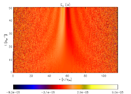
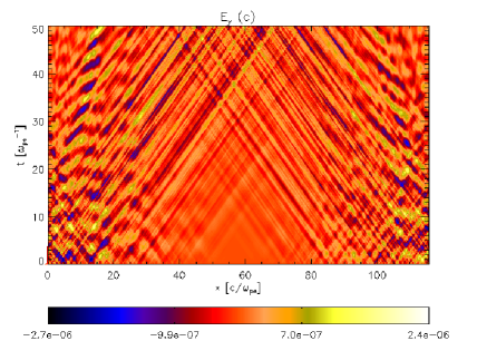
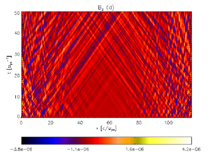
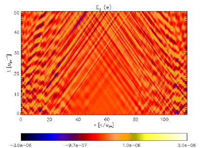
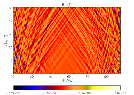
Figure 1: Time-distance plots for: (a) $E_{x}$, (b) $n_{e}-n_{e0}$, (c) $E_{y}$, (d) $B_{z}$, (e) $E_{z}$ and (f) $B_{y}$. This figure pertains to Section III.a.

In this section we present an equilibrium test run where the above described initial conditions are evolved for $50\omega_{pe}^{-1}$ without imposing an electron beam. The results are presented in Figure 1 where we show time-distance plots for the electrostatic (longitudinal to both background magnetic field and density gradient) electric field $E_{x}$ 1(a) and associated density perturbation, $n_{e}-n_{e0}$ 1(b); and two components of the transverse electromagnetic fields: ($E_{y}$ 1(c), $B_{z}$ 1(d)) and ($E_{z}$ 1(e), $B_{y}$ 1(f)). We gather from Figures 1(a) and 1(b) that only low level noise (with amplitudes $\sim 9\times 10^{-5}$ for $E_{x}$ and $\sim 3\times 10^{-2}$ for $n_{e}-n_{e0}$) is generated. This can be attributed to so called ”shot noise” that is normally present in PIC simulations. Figures 1(c)–1(f) demonstrate that in the electromagnetic emission component also low level (with amplitudes few $10^{-6}$) drift EM wave noise is generated. This can be evidenced by the fact that the slope of bright and dark strips is roughly the speed of light. Hence the perturbations are travelling with the speed of light. Note that the perturbations are generated in all parts of the density gradient but they are more prominent in the densest parts of the simulation domain, because their amplitudes are also expected to be largest there. No regular perturbations of longitudinal magnetic field ($B_{x}-B_{0x}$) are found (not shown here). Thus, we conclude that the equilibrium without the electron beam is fairly stable (apart from the low level EM drift wave noise).

III.2 Inhomogeneous plasma with electron beam injected along the magnetic field ($\theta=0^{\circ}$)

  

  

  

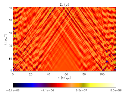
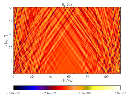
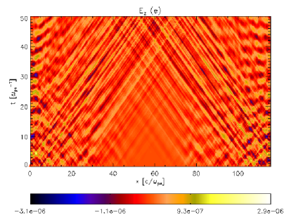
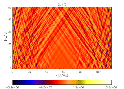
Figure 2: Time-distance plots for: (a) $E_{x}$, (b) $n_{b}$, the electron beam number density, (c) $E_{y}$, (d) $B_{z}$, (e) $E_{z}$ and (f) $B_{y}$. Here the beam pitch angle $\theta=0$. This figure pertains to Section III.b.

In this section we present the results when we inject the electron beam along the background magnetic field ($\theta=0^{\circ}$), where $\theta$ is the beam pitch angle (the angle between the initial beam velocity/momentum vector and the direction of background magnetic field). Here in Eq.(4) at $t=0$ we set $p_{0x}=0.5\gamma m_{e}c$ and $p_{0y}=0$. Note that in all cases with the injected beam we solve the initial value problem, i.e. electron beam initial drift momentum is applied only at $t=0$ – we do not re-inject the beam at every time step. The results are shown in Figure 2 where physical quantities shown are similar to that of Figure 1 except for 1(b) where instead we now present the time-distance plot for the electron beam, $n_{b}$. The reason why we have chosen to trace the dynamics of $n_{b}$ rather than full electron number density perturbation (background electron population plus the beam) is because as it was show in Section 2.3 of Ref.Tsiklauri (2010), when the beam is relatively dense ($n_{b}/n_{e}\approx$ few $10^{-2}$), the electron number density perturbation is dominated by a wake created by the beam. In Ref.Tsiklauri (2010) it was shown that when an electron beam, with the properties similar to considered here, is injected perpendicular to the background magnetic field, the beam excites electrostatic, standing waves, oscillating at local plasma frequency, in the beam injection spatial location. Here physical situation is different in that now the beam is injected along the magnetic field which is more plausible for the type III radio bursts. However, surprisingly we still see in Figure 2(a) the similar effect, that the standing ES waves are generated in the beam injection location. We can estimate the oscillation frequency by counting bright yellow strips in the region $2c/\omega_{pe}<x<8c/\omega_{pe}$ which is seven starting from the first strip. The time elapsed is $50\omega_{pe}^{-1}$, thus $50/2\pi=7.96$ and the conclusion is that this standing wave has approximately the plasma frequency. Note that the small mismatch is due to the fact that $\omega_{pe}$ in all normalisations is taken at the edges of the simulation domain where $n_{0}(0)=n_{0}(x_{max})=1$, while the beam injection location is centred on $x_{max}/25$ where $n_{0}(x_{max}/25)=0.846$. (The beam spatial spread here is within $2c/\omega_{pe}<x<8c/\omega_{pe}$). In Figure 2(a) $10c/\omega_{pe}<x<35c/\omega_{pe}$ we see series of oblique strips which is ES wake created by the beam. This can be evidenced by the fact that slope of these oblique strips is $(35-10)(c/\omega_{pe})/(50/\omega_{pe})=0.5c$ which coincides with the electron beam injection speed. Similar conclusion is reached from Figure 2(b) as well where the inferred slope of the beam is the same ($0.5c$). Note that for the times $t>30\omega_{pe}^{-1}$ there is small dip formed on the top of the beam (see Figure 2(b)). However the beam seems to stay intact which would be expected in the quasilinear theory (due to so called beam free streaming). This is despite the fact that $n_{b}/n_{e}=10^{-3}$ and the criterion of weak turbulence regime of quasilinear theory $\varepsilon\equiv n_{b}m_{e}v_{b}^{2}/(n_{0}m_{e}v_{th,e}^{2})\ll 1$ Mel’Nik et al. (1999) is actually not met: In our case $\varepsilon=4.94$ and also the quasilinear relaxation time, $\tau$, (time of establishing the plateau in the electron longitudinal velocity distribution function) is given by $\tau=n_{e}/({n_{b}}\omega_{pe})$ (e.g. Mel’Nik et al. (1999)). In our cause $\tau=10^{3}\omega_{pe}^{-1}$. Thus, no substantial quasilinear relaxation is expected to take place within $50\omega_{pe}^{-1}$. We gather from Figures 2(c)–2(f) as in Section III.a that only low level EM drift wave noise is generated and we see no generation of regular EM waves, commensurate to type III bursts. As discussed in the Introduction section when the beam pitch angle is zero then no EM waves should be generated; and it is only for the oblique pitch angles the EM emission generation is possible because then $\vec{v}_{b}\cdot\vec{E}_{\perp}\not=0$.

III.3 Inhomogeneous plasma with electron beam injected obliquely to the magnetic field ($\theta=45^{\circ}$)

  

  

  

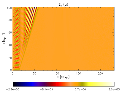
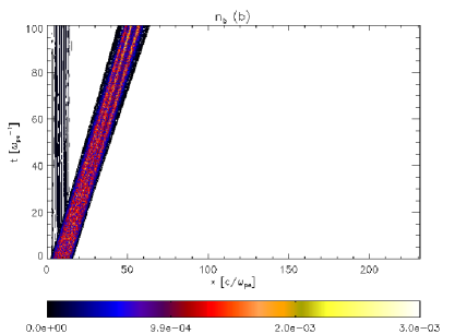
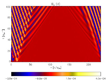
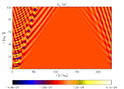
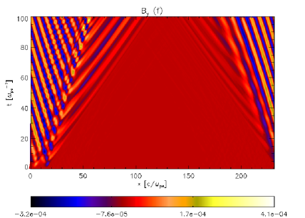
Figure 3: As in Figure 2 but for the beam pitch angle $\theta=45^{\circ}$. This figure pertains to Section III.c.

In this section we present results when we inject the electron beam obliquely to the background magnetic field ($\theta=45^{\circ}$). Here this is achieved by setting $p_{0x}=0.5\gamma m_{e}c$ and $p_{0y}=0.5\gamma m_{e}c$ in Eq.(4) at $t=0$. Note that since we intended to consider a numerical run for a twice longer time ($100\omega_{pe}^{-1}$) than in other above Sections, we have doubled the spatial domain size whilst keeping the same total number of particles $1.30065\times 10^{9}$. This implies that now the spatial grid size is $\lambda_{D}/2$, not $\lambda_{D}/4$ as in other above Sections. We gather from Figure 3(a) that again in the beam injection spatial location standing ES wave oscillating at local plasma frequency is excited. However, the ES wake of the beam, oblique yellow lines between $30c/\omega_{pe}<x<65c/\omega_{pe}$, detaches from the standing ES wave and becomes localised. The ES wake also travels with the correct speed of $\approx 0.5c$. Similar conclusions can be reached from analysing Figure 4(a) which reveals more detailed spatial structure of the ES wave oscillation and the ES beam wake. Figure 3(b) corroborates the beam travel speed of $0.5c$ as well as reveals minor deviation from the quasilinear theory free streaming, by appearance of spikes on the top of the beam. Figures 3(c)–3(f) present time-distance plots for the two components of the transverse electromagnetic fields: ($E_{y}$ 3(c), $B_{z}$ 3(d)) and ($E_{z}$ 3(e), $B_{y}$ 3(f)). We learn that as the beam pitch angle now is $\theta=45^{\circ}\not=0$ escaping EM radiation is generated. In the beam injection spatial location, $4c/\omega_{pe}<x<15c/\omega_{pe}$, we see strong interference pattern between the standing (trapped) ES and escaping EM radiation. The EM waves travel in both directions, and because of the periodic boundary conditions, waves that travel to the left, appear on the right side of the simulation domain ($x>150c/\omega_{pe}$). Figure 4(c) shows normalised electron number density at $t=100\omega_{pe}^{-1}$ (thick solid curve), beam spatial profiles at $t=0$ (dashed curve) and $t=100\omega_{pe}^{-1}$ (thin sold curve). Note that when plotting the spatial profiles of $n_{b}$, we scale it by a factor of $10^{3}$ so that it is clearly visible. We gather that the background electron population number density stays unchanged throughout the simulation, compared to $t=0$. This serves as additional proof that our initial conditions without the beam are stable. Also, comparing Figures 4(a) and 4(c) we confirm that indeed the beam and ES wake travel the same distance at the same speed of $\approx(65-15)c/\omega_{pe}/(100/\omega_{pe})=0.5c$. Figures 4(b) and 4(d) show a more detailed spatial structure of the transverse, escaping EM radiation components. We gather that these actually consist of two parts: (i) the part within $0<x<65c/\omega_{pe}$ corresponds to the non-escaping ES standing waves and the ES wake of the beam; and (ii) the part within $65c/\omega_{pe}<x<115c/\omega_{pe}$ that corresponds to the escaping EM radiation. Figures 4(e) and 4(f) show electron (including the electron beam) and ion longitudinal velocity distribution function time evolution. The considered momentum range is $3v_{th,i}m_{i}$, which is then converted to the velocities (in the relevant Figures) by using $3v_{th,i}m_{i}/(\gamma m_{e,i}c)$. We gather from Figure 4(e) that background electron population distribution remains unchanged (dashed ($t=0$) and solid ($t=100\omega_{pe}^{-1}$) curves, centred on $v_{x}=0$ do overlap to a plotting accuracy), while the electron beam starts to show a tendency of plateau formation, according to the quasi-linear theory. Note that in this Section simulation end time is 100 $\omega_{pe}^{-1}$ while the quasi-linear relaxation time is 1000 $\omega_{pe}^{-1}$. Recall however that we are not strictly speaking in the quasi-linear regime because $\varepsilon\approx 5$. The ion distribution function (Figure 4(f)) shows no noticeable by-eye change. Thus despite the fact that ions in the simulation are treated as mobile, the ion population shows no dynamics in the velocity space.

Next we attempt to produce a synthetic (simulated) dynamical spectrum. We take a snapshot of the spatial profile of one of the transverse EM components, $E_{y}(x,t=100\omega_{pe}^{-1})$, and cast it into the temporal dependence by putting $x=ct$. Thus in Figure 5(a) we see the same pattern in $E_{y}$ as in Figure 4(b) but now it appears as function of $t$ normalised to $\omega_{pe}^{-1}$. Note that we do not include EM wave which appear on the right due to the periodic boundary condition, i.e. we restrict ourselves to the range $x=[0,128c/\omega_{pe}]$ (i.e. the same as $t=[0,128\omega_{pe}^{-1}]$). We then generate a wavelet power spectrum for the $E_{y}(t)$. Wavelet software was provided by C. Torrence and G. Compo, and is available at URL: http://atoc.colorado.edu/research/wavelets/. We gather from Figure 5(b) that in the time interval $0<x<65\omega_{pe}^{-1}$ the wavelet power spectrum is flat (period/frequency does not change in time). This corresponds to ES oscillation part, oscillating at the plasma frequency (with a prefactor of $2\pi$). In the time interval $65<x<128\omega_{pe}^{-1}$ wavelet power spectrum corresponds to escaping EM radiation part and we clearly see a decrease of EM signal frequency in time. One has to realise however that in the Figure 5(b) it appears that large period $P_{LF}=15/(2\pi)$ (low frequency) at $t\approx 65\omega_{pe}^{-1}$ shows up first and then low period $P_{HF}=9/(2\pi)$ (high frequency) at $t\approx 115\omega_{pe}^{-1}$ follows. This has a simple explanation that we obtained the time series of $E_{y}$ by putting $x=ct$. In reality for a distant observer located in a point, the high frequency (high density) would appear first followed by a low frequency radio signal. Note also that the frequency decrease nicely follows the number density decrease. In Figure 4(c) dashed line peak which represents the beam at $t=0$ is located at the normalised background electron number density (thick solid line) of 0.846. By the time beam reaches its final destination by time $t=100\omega_{pe}^{-1}$ (thin solid line) the density has dropped to $\approx 0.3$. Therefore we would have expected that the corresponding plasma frequency has dropped by a factor $\sqrt{0.3/0.846}=0.595$. Indeed we gather from Figure 5(b) that $P_{HF}/P_{LF}=9/15=0.6$. In other words, $\omega_{p,LF}/\omega_{p,HF}=\sqrt{n_{LF}/n_{HF}}=\sqrt{0.3/0.846}=0.595\approx P_{HF}/P_{LF}=9/15=0.6$, where the notation is straightforward. Therefore we conclude that the frequency decrease in the synthetic dynamical spectrum is commensurate to the plasma frequency (electron number density) decrease along the beam propagation path. Note that it is only in the interplanetary type III radio bursts the frequency drops by many orders of magnitude. However, the bursts that occur in the solar corona show frequency drops by about a factor of two (as in our simulation), are not uncommon. For example decameter type II bursts which have a fine structure in the form of type III-like bursts. The drift rates of these sub-bursts are close to the ordinary type III bursts velocity, but their duration is essentially lesser Mel’nik et al. (2004).

Figure 4: (a) $E_{x}(x,t=100\omega_{pe}^{-1})$, (b) $E_{y}(x,t=100\omega_{pe}^{-1})$, (c) $n_{e}(x,t=100\omega_{pe}^{-1})$ (thick solid curve), $n_{b}(x,t=100\omega_{pe}^{-1})$ (thin solid curve), $n_{b}(x,t=0)$ (dashed curve) (Note that $n_{b}$ is scaled by a factor of $10^{3}$ so that it is clearly visible.), (d) $B_{z}(x,t=100\omega_{pe}^{-1})$, (e) background and beam electron longitudinal ($v_{x}$) velocity distribution functions $f_{e}(v_{x},t=100\omega_{pe}^{-1})+f_{b}(v_{x},t=100\omega_{pe}^{-1})$ (solid curve) and $f_{e}(v_{x},t=0)+f_{b}(v_{x},t=0)$ (dashed curve), (f) ion longitudinal ($v_{x}$) velocity distribution functions $f_{i}(v_{x},t=100\omega_{pe}^{-1})$ (solid curve) and $f_{i}(v_{x},t=0)$ (dashed curve) (Note that to a plotting precision the two curves overlap). This figure pertains to Section III.c.

Figure 5: (a) Time evolution of $E_{y}$ (see text how spatial $x$-dependence was cast into time $t$-dependence), (b) wavelet power spectrum of (a). This figure pertains to Section III.c.

III.4 Homogeneous plasma with electron beam injected obliquely to the magnetic field ($\theta=45^{\circ}$)

  

  

  

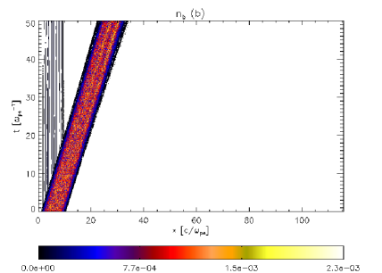
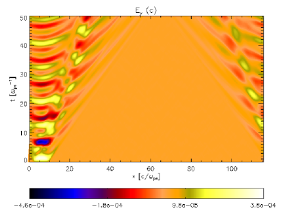
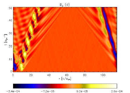
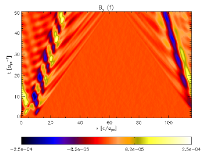
Figure 6: As in Figure 2 but for the beam pitch angle $\theta=45^{\circ}$ and homogeneous background number density. This figure pertains to Section III.d.

Figure 7: (a) $E_{x}(x,t=50\omega_{pe}^{-1})$, (b) $E_{y}(x,t=50\omega_{pe}^{-1})$, (c) $n_{e}(x,t=50\omega_{pe}^{-1})$ (thick solid line), $n_{b}(x,t=50\omega_{pe}^{-1})$ (thin solid curve), $n_{b}(x,t=0)$ (dashed curve) (Note that $n_{b}$ is scaled by a factor of $10^{3}$ so that it is clearly visible.), (d) $B_{z}(x,t=50\omega_{pe}^{-1})$, (e) background and beam electron longitudinal ($v_{x}$) velocity distribution functions $f_{e}(v_{x},t=50\omega_{pe}^{-1})+f_{b}(v_{x},t=50\omega_{pe}^{-1})$ (solid curve) and $f_{e}(v_{x},t=0)+f_{b}(v_{x},t=0)$ (dashed curve), (f) ion longitudinal ($v_{x}$) velocity distribution functions $f_{i}(v_{x},t=50\omega_{pe}^{-1})$ (solid curve) and $f_{i}(v_{x},t=0)$ (dashed curve) (Note that to a plotting precision the two curves overlap). This figure pertains to Section III.d.

In this section we present the results when we inject the electron beam obliquely to the background magnetic field ($\theta=45^{\circ}$) as in Section III.c. However, contrary to the Section III.c here we consider a plasma with uniform background number density $n_{0}=1$. We see from Figure 6(a) that as in Section III.c in the location where the beam was injected standing ES waves are generated, oscillating at local plasma frequency. However, as better seen from Figure 7(a) now the ES wake created by the beam does not have enough time to detach itself from the standing wave. This is due to the fact that this is a shorter run ($t_{end}=50\omega_{pe}^{-1}$). We also gather from Figures 6(b) and 7(c) that the beam travels the correct distance, commensurate to its speed. Figures 6(c)–6(f) show time distance plots of transverse EM components that are generated by the Langmuir (ES) waves. Their more detailed spatial profiles are shown in Figures 7(b) and 7(d). It is evident by eye that in the uniform plasma case there is no frequency decrease with time for the generated EM components. Therefore we do not produce the synthetic dynamical spectrum as in Section III.c. Figures 7(e) confirms that the predictions of the quasilinear theory, that by time $t=50\omega_{pe}^{-1}$ we see (i) no noticeable quasi-linear relaxation because the plateau is expected to develop in quasi-linear relaxation time of 1000 $\omega_{pe}^{-1}$; (ii) electron free streaming is also evident. No noticeable change in ion velocity distribution function is seen either. Note that the escaping EM radiation is generated in the uniform plasma density case too. This indicates that the density gradient plays no role in the EM emission generation.

III.5 Inhomogeneous plasma with electron beam injected obliquely to the magnetic field ($\theta=45^{\circ}$), weak magnetic field case

In this Section we consider the case similar to III.c but with ten times weaker magnetic field, $B=3$ gauss, such that $\omega_{ce}/\omega_{pe}(x=0)=0.094$, unlike in the rest of the paper where $\omega_{ce}/\omega_{pe}(x=0)=0.94$ (which is more appropriate to solar coronal conditions). This is to unambiguously demonstrate that the present study is indeed relevant for the type III radio burst emission, via the 1.5D non-zero pitch angle (non-gyrotropic) electron beam quasilinear relaxation, and subsequent emission at the plasma frequency rather than the electron gyro-frequency emission. In the laboratory plasma there are microwave generation devices, such as Gyrotron, in which EM radiation is produced at electron gyro-frequency, $\omega_{ce}$. At first sight, it would seem probable that since for the considered model parameters throughout this paper $\omega_{ce}/\omega_{pe}(x=0)=0.94$, what we report is the Gyrotron type EM radiation. The issue can be settled by e.g. lowering the magnetic field value. The results are presented in Figs. 8-10, which are mirror analogs to Figs.3-5, except that here $\omega_{ce}/\omega_{pe}(x=0)=0.094$. We gather from Fig.8a that the generated ES (Langmuir) component behaviour is nearly identical to that of Fig.3a, i.e. we again see the generation of standing ES waves, oscillating at plasma frequency, $\omega_{pe}$, in the beam injection spatial location, $4c/\omega_{pe}<x<15c/\omega_{pe}$. The electron beam dynamics is also identical (cf. Fig.8b and Fig.3b). There are notable differences in the generated transverse to the magnetic field EM components: By comparing Figs.8c–8f to Figs.3c–3f, we see that in the escaping EM ration there is no interference pattern, i.e. there is no interference between the standing (trapped) ES and escaping EM radiation. This is because now ES oscillation no longer appears in $E_{y}$, $E_{z}$, $B_{y}$, and $B_{z}$ transverse EM components. What is crucial that in the time-distance plots, Figs.8c–8f, we still see the same number of bright (and dark) strips, which is indicative of the fact that the escaping EM radiation oscillates again at approximately plasma frequency, $\omega_{pe}$, and not at electron cyclotron frequency $\omega_{ce}$.

  

  

  

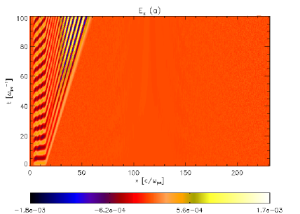
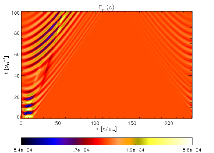
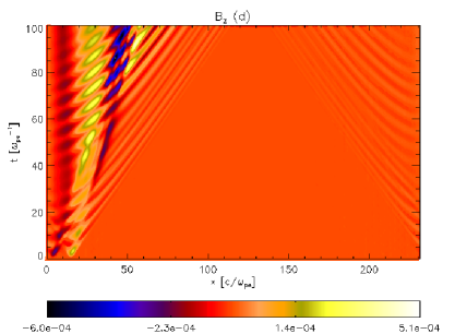
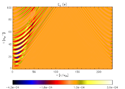
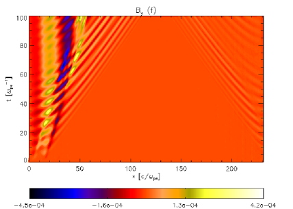
Figure 8: As in Figure 3 but for 10 times weaker magnetic field such that $\omega_{ce}/\omega_{pe}(x=0)=0.094$. This figure pertains to Section III.e.

We gather from Fig.9, which corresponds closely to Fig.4, but here $\omega_{ce}/\omega_{pe}(x=0)=0.094$, that most of the conclusions reached when considering Fig. 4 apply here too. However, a notable difference is that by comparing Figs.4b and 9b we deduce that in transverse electric field component $E_{y}$, for $0<x<65c/\omega_{pe}$, we no longer see the standing (trapped) ES component, i.e. only the escaping EM radiation is present.

Figure 9: As in Fig.4 but for 10 times weaker magnetic field such that $\omega_{ce}/\omega_{pe}(x=0)=0.094$. This figure pertains to Section III.e.

Fig.10 has been produced in the same way as Fig.5, except that now $\omega_{ce}/\omega_{pe}(x=0)=0.094$. We gather from Fig.10 that, contrary to Fig.5 in which both the ES oscillation and escaping EM component were present, now we see only escaping EM wave which clearly shows the drift towards lower frequencies. We also observe that as in Fig.5, $\omega_{p,LF}/\omega_{p,HF}\approx 0.6$ that is commensurate to the background plasma density decrease.

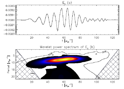
Figure 10: As in Fig.5 but for 10 times weaker magnetic field such that $\omega_{ce}/\omega_{pe}(x=0)=0.094$. This figure pertains to Section III.e.

IV Conclusions

A quote from Melrose (1999), p.95, summarises the state of the matters in theoretical understanding of solar type III radio bursts rather well: ”Our understanding of plasma emission is in an unsatisfactory state. It seems that the problems with our understanding of plasma emission are of an astrophysical nature and will eventually be solved through new observational data. There are several different possible mechanisms which can lead to fundamental plasma emission and it is still not clear which is the relevant one in practice. Although this leaves the theory of fundamental plasma emission in a somewhat uncertain state, the theory for second harmonic is well understood; there seems to be no reasonable alternative for the coalescence process $L+L\to T$”. Also Introduction section of Ref. Malaspina et al. (2010) provides a good, critical overview of the possible mechanisms which generate the type III burst EM radiation. These include, (i) the classical plasma emission mechanism that is based on non-linear wave-wave interaction between Langmuir, ion-acoustic and EM waves; (ii) a linear mode conversion, in which almost monochromatic Langmuir z-mode interacts with the density gradient, partly reflecting and partly converting into the EM radiation; (iii) the quasimode mechanism in which forward- and backward- propagating Langmuir waves generate a quasinormal electrostatic mode at $2\omega_{pe}$ which further converts into EM harmonic radiation and (iv) the antenna radiation model which involves direct radiation of charged particles that oscillate at $\omega_{pe}$ and drive currents at $2\omega_{pe}$. In this work we presented the results which show that 1.5D non-zero pitch angle (non-gyrotropic) electron beam can also produce escaping EM radiation at $\omega_{pe}$ which seems to successfully mimic the observed solar type III radio bursts. A clear distinction needs to be drawn between the best studied type III burst mechanism, the classical plasma emission Ginzburg and Zhelezniakov (1958), and the model presented in this work. In the plasma emission mechanism non-linear wave-wave interaction between Langmuir, ion-acoustic and EM waves requires that the beat conditions $\omega_{1}+\omega_{2}=\omega$ and $\vec{k}_{1}+\vec{k}_{2}=\vec{k}$ to be satisfied. The emission formula (i.e. the three wave interaction probability) for the relevant process $L+s\to T$ (coalescence of Langmuir and ion-sound wave to produce transverse EM wave) includes a cross vector product factor $|\vec{k}_{L}\times\vec{k}_{T}|^{2}$ (see e.g. Eqs.(26.24) and (26.25) from Ref.Melrose and McPhedran (2005). This implies that, whilst electron beam and Langmuir turbulence dynamics can be treated in 1D spatial dimensions (and there is large body of work that deals with the 1D quasilinear theory), the correct treatment of act of EM emission needs 2D spatial dimensions. This is because in 1D case the factor $|\vec{k}_{L}\times\vec{k}_{T}|^{2}$ is identically zero, because the angle between wave vectors of Langmuir wave, $\vec{k}_{L}$, and EM wave, $\vec{k}_{T}$, is zero. This has to be distinguished from the pitch angle $\theta$ which in our notation is the angle between the particle (electron) beam injection direction and the background magnetic field. We remark however that the plasma emission mechanism equations use ”random phase approximation” (see e.g. p.383 from Ref.Melrose and McPhedran (2005)). This is because the extraneous, quadratic non-linear current (see their Eq.(26.2)) depends on the phases of the beating fields and some assumption needs to be made concerning the phase. A priori, it is not at all clear that in the case of our situation, in which non-zero pitch angle (non-gyrotropic) electron beam is injected, the phases are random. Hence whether the factor $|\vec{k}_{L}\times\vec{k}_{T}|^{2}$ is applicable in our case. Without further in-depth analysis it would be safe to conclude that our simulations do not involve the classical plasma emission processes.

We have performed-high resolution (sub-Debye length grid size and 10000 particle species per cell), 1.5D Particle-in-Cell, relativistic, fully electromagnetic simulations to model electromagnetic wave emission generation in the context of solar type III radio bursts. We studied the generation of EM waves by injecting a super-thermal, hot beam of electrons into a plasma thread that contains uniform longitudinal magnetic field and a parabolic density gradient along the magnetic field. We have considered five cases:

(i) As an initial equilibrium test, we find that the physical system without electron beam is stable and only low amplitude level electromagnetic drift waves (noise) are excited.

(ii) The beam injection direction is then controlled by setting either longitudinal or oblique initial electron drift speed/momentum. i.e. we set different beam pitch angles. In the case of zero beam pitch angle, i.e. when $\vec{v}_{b}\cdot\vec{E}_{\perp}=0$, the beam excites only ES standing waves, oscillating at local plasma frequency. This oscillation occurs strictly in the beam injection spatial location and only low level electromagnetic drift wave noise is present (no regular EM waves are generated by the beam).

(iii) In the case of oblique beam pitch angle, i.e. when $\vec{v}_{b}\cdot\vec{E}_{\perp}\not=0$ again ES waves with similar properties are excited. In this case however because the beam can interact with the EM waves, it generates EM waves with the properties commensurate to type III radio bursts. In particular, wavelet analysis of transverse electric field component shows that as the beam moves to the regions of lower density and hence lower plasma frequency, EM wave frequency drops accordingly.

(iv) When we remove the density gradient, an electron beam with an oblique pitch angle still generates the EM radiation, but now no frequency decrease is produced.

(v) In order to prove that the generated, by the non-zero pitch angle beam, EM emission oscillates at the plasma frequency, we also consider a case when the magnetic field (and hence the cyclotron frequency) is ten times smaller.

Using fully kinetic plasma model our results also broadly confirm (i) the fact that in order to excite escaping EM waves, the electron beam should have non-zero pitch angle; i.e. there should be a non-zero projection of the electron beam injection velocity vector on the transverse EM electric field vector. (ii) quasilinear theory predictions, namely quasilinear relaxation time-scale and free streaming assumptions were corroborated via fully kinetic simulation, in a realistic to the type III burst magnetic field geometry. (iii) The observational fact that there should be a EM emission frequency drift in time in the inhomogeneous plasma case has been also confirmed via production of the simulated (synthetic) dynamical spectrum for the first time.

The presented model will be used in the future for the forward modelling of the observed type III burst dynamical spectra (2D radio emission intensity plots where frequency is on $y$-axis and time on $x$-axis). The main forward modelling goal will be inferring the electron number density profile along the beam propagation paths.

We would like to close by pointing out some pertinent limitations of the considered model in its direct applicability to the solar type III radio burst observations. The issues are:

(i) In the solar type III bursts, electron beams propagate large distances without being depleted by the generated Langmuir waves due to bump-on-tail instability (also called beam-plasma instability). In the linear regime, the timescale for the quasilinear relaxation, $\tau=n_{e}/({n_{b}}\omega_{pe})$ and hence timescale of the beam depletion is prescribed by the ratio of the electron beam and background plasma densities. To be precise, $\tau$ is the inverse of the linear bump-on-tail instability growth rate $\gamma=\omega_{pe}(n_{b}/n_{e})(v_{b}^{2}/\delta v_{b}^{2})$, where $\delta v_{b}$ is the electron beam velocity thermal spread. Thus for $v_{b}\approx\delta v_{b}$, $\tau\approx 1/\gamma$. Due to the above described computational limitations, at present, it was impractical to set $n_{b}/n_{e}$ to the observed values $10^{-5}-10^{-8}$; This may affect the process of beam (re-)generation by the time-of-flight effects; Also, it is known that electron beam may be stabilised by non-linear effects Tsytovich and Shapiro (1965). In the non-linear stimulated scattering processes, the wavenumbers are drawn out of the resonance. This leads to energy transfer rate between the beam electrons and Langmuir wave at a much slower rate than quasilinear relaxation time, that effectively leads to the non-linear stabilisation of the bump-on-tail instability. For the parameters commensurate to the type III bursts, the condition for the stabilisation, $n_{b}/n_{e}\ll{v_{th,e}^{4}}/{v_{b}^{4}}\ll(m_{e}/m_{i})(\delta v_{b}/v_{b})$ is met in most cases. Therefore the non-linear stabilisation is likely to play a major role. (e.g. Ref.Tsytovich (1995), pp.184-187 or Tsytovich and Shapiro (1965))

(ii) The spatial scale of the density gradient (decrease of $\omega_{pe}$ by a factor of $10^{4}$ over 65,000 Debye length) is not realistic (we have to remember that in PIC simulations one uses a smaller than in reality number of ”super-particles” and not real electrons and protons). This may affect criteria for onset of instabilities caused by plasma density inhomogeneities; For example, when the electron beam moves along the density gradient, Langmuir wave phase velocity will change while the beam velocity remains constant when there is no strong relaxation Ryutov (1970). If the instability growth rate is much less than the reciprocal of the time of escape from the resonance, the beam stabilises as it no longer loses energy to the wave generation. The condition for the stabilisation is $L<(n_{e}/n_{b})(3v_{th,e}^{2}/(v_{b}\omega_{pe}))$, where $L$ is the characteristic spatial scale of the plasma density inhomogeneity (see e.g. Ref.Kaplan and Tsytovich (1973), p. 119). For the broad range of the solar coronal conditions as well as for the set of parameters considered in this paper (from Figure 4c, thick sold curve, we see that plasma density drops by a factor of 2 over a length scale of $L\approx 30c/\omega_{pe}$, whereas $(n_{e}/n_{b})(3v_{th,e}^{2}/(v_{b}\omega_{pe}))=0.3c/\omega_{pe}$) the latter inequality is not met.

(iii) Moreover the observed electron beam pitch angles are also much smaller Reiner et al. (2009) than considered in the present model. Despite these limitations, the present model provides a proof-of-concept for the EM emission generation in the context of type III solar radio bursts.

On a positive note, the considered regime may provide an important diagnostic to laboratory laser plasma or thermonuclear fusion studies as in both cases non-thermal beams of electrons are frequently present.