CaCu₂(SeO${}_{3})_{2}$Cl₂: spin-$\frac{1}{2}$ Heisenberg chain compound with complex frustrated interchain couplings

Abstract

We report the crystal structure, magnetization measurements, and band-structure calculations for the spin-$\frac{1}{2}$ quantum magnet CaCu₂(SeO${}_{3})_{2}$Cl₂. The magnetic behavior of this compound is well reproduced by a uniform spin-$\frac{1}{2}$ chain model with the nearest-neighbor exchange of about 133 K. Due to the peculiar crystal structure, spin chains run in the direction almost perpendicular to the structural chains. We find an exotic regime of frustrated interchain couplings owing to two inequivalent exchanges of 10 K each. Peculiar superexchange paths grant an opportunity to investigate bond-randomness effects under partial Cl–Br substitution.

I Introduction

Low-dimensional magnets remain an attractive playground to study quantum phenomenaBalents (2010) and to understand strongly correlated electronic systems on a model level.Lee (2008) Theoretical investigations disclose interesting features of numerous simple spin networks, such as a diamond chain,Takano et al. (1996) a kagomé lattice,Hastings (2000) or a pyrochlore lattice.Canals and Lacroix (1998) The transfer of these spin lattices to real systems and the subsequent experimental verification of theoretical results are, however, rather problematic and stimulate extensive studies of low-dimensional (or potentially low-dimensional) magnetic materials. Most of these studies are focused on Cu⁺² compounds, because the $d^{9}$ nature and the pronounced Jahn-Teller effect of Cu⁺² ion lead to insulating spin-$\frac{1}{2}$ compounds with diverse spin-lattice geometries.

Aiming to find hitherto unexplored examples of low-dimensional spin systems, we investigate copper selenite-chlorides. These compounds combine two important structural ingredients that lead to unusual physical behavior: i) SeO₃ selenite groups contain the lone-pair Se⁺⁴ cation that induces exotic (and potentially polar) crystal structures, as in the piezoelectric ferrimagnet Cu₂OSeO₃ (Refs. Bos et al., 2008; *cu2oseo3_nmr); ii) Cl atoms show strong hybridization with Cu $3d$ orbitals and mediate long-range exchange couplings, leading to highly entangled spin lattices in spin-tetrahedra compounds Cu₂Te₂O₅X₂ (X = Cl, Br)Zaharko et al. (2006) showing incommensurate magnetic order, or in the intricate spin-dimer system (CuCl)LaNb₂O₇ (Ref. Tsirlin and Rosner, 2009, 2010).

Here, we present an experimental and computational study of CaCu₂(SeO${}_{3})_{2}$Cl₂. X-ray diffraction, magnetization measurements, and band structure calculations are applied to elucidate crystal structure, electronic structure, and magnetic behavior of this compound. In our study, the complex structural arrangement of Cu polyhedra is readily disentangled by a microscopic approach. We find the conventional $x^{2}-y^{2}$ orbital ground state for both Cu sites, and establish a minimum magnetic model of uniform spin-1/2 chains with weak, frustrated interchain couplings.

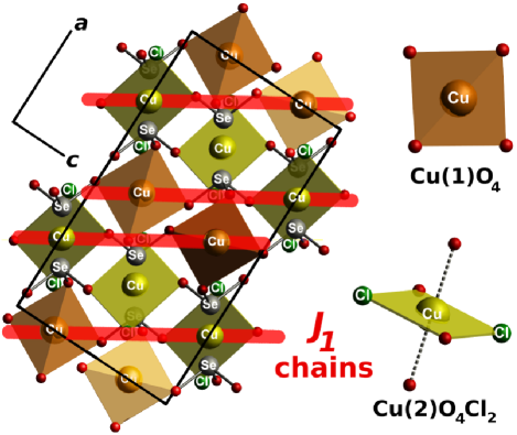
Figure 1: (Color online) Left: crystal structure of CaCu₂(SeO${}_{3})_{2}$Cl₂. The structural chains run along $[10\bar{1}]$ (not shown), whereas the magnetic chains range along $\sim[201]$, as shown by bold (red) lines. Small unlabeled spheres denote O atoms. Right: local environment of Cu(1) and Cu(2). The magnetically active Cu(1)O₄ and Cu(2)O₂Cl₂ plaquettes are highlighted.

II Synthesis and sample characterization

Calcium selenite CaSeO₃ was prepared via solution synthesis, as described in Ref. Dityatiev et al., 2007. The solutions of calcium nitrate Ca(NO${}_{3})_{2}$ (chemically pure) (6.214 g) and selenous acid H₂SeO₃ (98 %) (4.886 g) in a minimal amount of hot distilled water were mixed. The ammonia 1:5 water solution was added to fix pH of the solution in the range 7$-$8. The fine white powder was obtained as a precipitate. The precipitate was then dried at 150 ^∘C. According to X-ray powder diffraction (XRPD), the obtained powder was identified as a hydrate CaSeO${}_{3}\cdot$H₂O. The hydrate was further calcined on a gas burner in a ceramic plate for 30 min. The resulting product was identified as a single phase CaSeO₃ [space group $P2_{1}/n$, $a$ = 6.399(5) Å, $b$ = 6.782(4) Å, $c$ = 6.682(8) Å, $\beta$ = 102.84(6) ^∘].

SeO₂ was obtained from H₂SeO₃ by its decomposition under vacuum at 60 ^∘C and the sublimation of the resulting substance in a flow of anhydrous air and NO₂.

CuO (ultra pure) and CuCl₂ (Merck, $>$98 %) were used. The dark-greenish powder sample of CaCu₂(SeO${}_{3})_{2}$Cl₂ was obtained from a stoichiometric mixture of CaSeO₃, CuCl₂, CuO, and SeO₂. The mixture (about 0.5 g total) was prepared in Ar-filled camera, sealed in a quartz tube, and placed into the electronically controlled furnace. The sample was heated from room temperature to 300 ^∘C for 12 hours, exposed at 300 ^∘C for 24 hours, heated up to 500 ^∘C for 12 hours, and exposed at 500 ^∘C for 96 hours.

The resulting samples were single-phase, as confirmed by powder x-ray diffraction (STOE STADI-P diffractometer, CuK_α1 radiation, transmission geometry). The powder pattern was fully indexed in the monoclinic space group $C2/c$ with lattice parameters $a$ = 12.752(3) Å, $b$ = 9.036(2) Å, $c$ = 6.970(1) Å, $\beta$ = 91.02(1) ^∘. CaCu₂(SeO${}_{3})_{2}$Cl₂ is rather stable in air, although a prolonged exposure of about 3 months led to a partial decomposition towards crystalline CuSeO₃$\cdot$2H₂O and possible amorphous products.

Table 1: Data collection and structure refinement parameters for CaCu₂(SeO${}_{3})_{2}$Cl₂.

Parameter	Value
Temperature (K)	293(2)
Radiation, $\lambda$ (Å)	MoKα, 0.71069
Space group	$C2/c$ (No. 15)
$a$ (Å)	12.759(3)
$b$ (Å)	9.0450(18)
$c$ (Å)	6.9770(14)
$\beta$ (∘)	91.03(3)
$V$ (Å3)	805.1(3)
$Z$	4
Calculated density (g/cm3)	4.059
Absorption coefficient $\mu$ (mm-1)	15.612
Crystal size (mm)	$0.30\times 0.07\times 0.06$
Angle range (deg)	$2.76<\theta<31.96$
Index ranges	$-18{\leq}h{\leq}18$,
	$0{\leq}k{\leq}13$,
	$-10{\leq}l{\leq}2$
Reflections: total / independent	1512/1401
$R_{\text{int}}$	0.0171
Completeness to $\theta$ = 31.96 ∘	100.0 %
Absorption correction	$\psi$-scan corrections
Max./min. transmission	0.392/0.280
Parameters refined / restraints	63/0
Refinement method	full-matrix
	least-squares on $F^{2}$
Goodness of fit on $F^{2}$	1.016
$R_{1}$, $wR_{2}$ ($F_{o}>4\sigma(F_{o})$)	0.0279, 0.0761
$R_{1}$, $wR_{2}$ (all data)	0.0430, 0.0796
Extinction coefficient	0.00085(18)
Largest diff. peak and hole	$0.914,-1.188$

III Crystal structure

For the structure determination, a single crystal was picked up from the bulk polycrystalline sample. The data were collected at the CAD-4 (Nonius) diffractometer (MoK_α radiation) at room temperature. The analysis of systematic extinctions unambiguously pointed to the space group $C2/c$ (15). The lattice parameters $a=12.759(3)$ Å, $b=9.0450(18)$ Å, $c=6.9770(14)$ Å and $\beta=91.03(3)$ ^∘ were refined, based on 24 well-centered reflections in the angular range $12.01$ ^∘ $<$ $\theta$ $<$ 15.84 ^∘. The diffraction data were collected in an $\omega-2\theta$ mode with the data collection parameters listed in Table 1. A semiempirical absorption correction was applied to the data based on $\psi$-scans of seven reflections with $\lambda$ angles close to 90 ^∘.

Positions of metal and selenium atoms were found by direct methods (shelxs-97).Sheldrick (2008) Oxygen atoms were localized by a sequence of least-square cycles and difference Fourier syntheses $\Delta\rho(x,y,z)$. The final refinement with anisotropic atomic displacement parameters was based on $F^{2}$ (shelxl-97).Sheldrick (2008) Further information and the refinement residuals are given in Table 1. Atomic coordinates and atomic displacement parameters are listed in Table 2.

Table 2: Atomic coordinates and atomic displacement parameters $U_{\text{iso}}$.

Atom	Position	$x/a$	$y/b$	$z/c$	$U_{\text{iso}}$
Ca	$4e$	0	0.8425(1)	0.25	1.1(1)
Cu(1)	$4e$	0	0.6221(1)	0.75	1.2(1)
Cu(2)	$4c$	0.25	0.25	0	1.2(1)
Se	$8f$	0.1704(1)	0.6053(1)	0.0878(1)	0.8(1)
Cl	$8f$	0.6170(1)	0.5817(1)	0.1048(1)	1.7(1)
O1	$8f$	0.1609(2)	0.7153(3)	0.2852(4)	1.4(1)
O2	$8f$	0.0493(2)	0.6598(3)	0.0070(3)	1.3(1)
O3	$8f$	0.1455(2)	0.4342(3)	0.1704(4)	1.4(1)

The crystal structure of CaCu₂(SeO${}_{3})_{2}$Cl₂ is shown in Fig. 1. It comprises two inequivalent Cu positions (Table 2). The Cu(1) atoms show a slightly distorted square-planar Cu(1)O₄ environment, typical for Cu⁺² oxides (Table 3). In contrast, Cu(2) is six-fold coordinated, with four oxygens and two chlorines forming an octahedron, squeezed along Cu(2)–O1 (Table 3). Although such octahedral coordination of Cu(2) is rather unusual, it still allows for a square-planar-like crystal-field splitting of $3d$ levels and the conventional non-degenerate $3d^{9}$ orbital ground state with the half-filled $3d_{x^{2}-y^{2}}$ orbital lying in the plane of a Cu(2)O₂Cl₂ plaquette (Fig. 1). This plaquette is formed by two Cu(2)–Cl bonds and two Cu(2)–O1 bonds. The formation of the plaquette can be qualitatively understood in terms of different ionic radii for oxygen and chlorine. The larger size of the Cl atoms makes their effect on the Cu $3d$ orbitals similar to the effect of O1 with shorter distances to Cu. The resulting crystal-field splitting resembles that of a CuO₄ plaquette and drives one of the atomic $d$ orbitals half-filled as well as magnetic, that is $a$ $posteriori$ confirmed by our DFT calculations (Sec. V).

Table 3: Selected interatomic distances (in Å) in the CaCu₂(SeO${}_{3})_{2}$Cl₂ structure.

Atom pair	Distance		Atom pair	Distance
Ca–O1 ($\times{}2$)	$2.362(2)$		Cu(1)–O2 ($\times{}2$)	$1.920(2)$
Ca–O2 ($\times{}2$)	$2.458(3)$		Cu(1)–O3 ($\times{}2$)	$2.012(2)$
Ca–Cl ($\times{}2$)	$2.827(1)$
Ca–Cl ($\times{}2$)	$2.948(1)$		Cu(2)–O1 ($\times{}2$)	$1.891(2)$
Se–O1	1.705(2)		Cu(2)–O3 ($\times{}2$)	$2.455(2)$
Se–O2	1.707(2)		Cu(2)–Cl ($\times{}2$)	$2.404(1)$
Se–O3	1.684(3)

In general, the formation of CuO₂Cl₂ plaquettes is typical for copper oxychlorides.Tsirlin and Rosner (2010); Schmitt et al. (2009) However, a unique feature of CaCu₂(SeO${}_{3})_{2}$Cl₂ is the presence of two longer Cu(2)–O3 bonds which look similar to the Cu(2)–Cl bonds in terms of interatomic distances but are essentially inactive with respect to the magnetism, as will be shown in Sec. IV.

The Cu(1)O₄ plaquettes and the Cu(2)O₄Cl₂ octahedra share corners and form chains along $[10\bar{1}]$. However, the bridging O3 atoms do not belong to the Cu(2)O₂Cl₂ plaquettes, hence a simple Cu(1)–O3–Cu(2) superexchange is unlikely. Instead, the leading exchange couplings should run via SeO₃ trigonal pyramids which join the plaquettes into a framework. The Cl atoms shape tunnels that run along $c$ and accommodate the Ca cations. Surprisingly, CaCu₂(SeO${}_{3})_{2}$Cl₂ bears no relation to SrCu₂(SeO${}_{3})_{2}$Cl₂ (Ref. Berdonosov et al., 2009) owing to the smaller size of Ca and the high flexibility of Cu–Se–O–Cl framework. The arrangement of polyhedra does not resemble any known structure type either.

IV Magnetic properties

Magnetic susceptibility ($\chi$) of CaCu₂(SeO${}_{3})_{2}$Cl₂ was measured with a Quantum Design MPMS SQUID magnetometer in the temperature range $2-380$ K in applied fields $\mu_{0}H$ of 0.5, 2, and 5 T.

The $\chi(T)$ dependence (Fig. 2) shows a broad maximum at 83 K and a pronounced increase below 30 K. The susceptibility maximum is a signature of quantum fluctuations (low-dimensional and/or frustrated behavior), while the low-temperature upturn is caused by the paramagnetic contribution of defects and impurities. Above 230 K, we fit the data with the modified Curie-Weiss law $\chi$ = $\chi_{0}+C/(T+\theta)$ where $\chi_{0}$ = 6(1)$\times$10^-5 emu (mol Cu)^-1 accounts for the temperature-independent (e.g., van Vleck) contribution, $C$ = $0.42(1)$ emu K (mol Cu)^-1 is the Curie constant, and $\theta$ = 93(5) K is the Weiss temperature. The positive $\theta$ indicates predominant antiferromagnetic (AFM) interactions in the system. Using the expressions

$$C=\frac{N_{A}\mu_{\text{eff}}^{2}}{3k_{B}},\hskip 21.68231pt\mu_{\text{eff}}=g\mu_{B}\sqrt{S(S+1)}$$ (1)

we obtain the resulting effective magnetic moment $\mu_{\text{eff}}$ = $1.83(1)$ $\mu_{B}$ and the $g$-factor $g$ = $2.11(1)$, typical for spin-$\frac{1}{2}$ Cu⁺².Möller et al. (2009)

To fit the whole $\chi(T)$ dependence, we used different expressions for simple low-dimensional spin models. The best fit was obtained with the expression for the uniform spin-$\frac{1}{2}$ chain $\chi_{\text{ch}}$, given by Ref. Johnston et al., 2000 $[$see their Eq. (53) parameterized with the values provided in the third column of Table I$]$. The temperature range 2 $-$ 380 K fits to the validity condition of this parameterization 0 $\leq$ $J$ $\leq$5.Johnston et al. (2000) To account for temperature-independent and the low-temperature impurity contribution to $\chi(T)$, we supplemented $\chi_{\text{ch}}$ with the $\chi_{0}$ term and the Curie term $C_{\text{imp}}/T$, respectively:

$$\chi(T)=\chi_{0}+\dfrac{C_{\text{imp}}}{T}+\frac{N_{A}g^{2}\mu_{B}^{2}}{J}\,\chi_{\text{ch}}\left(\frac{T}{J}\right).$$ (2)

The fit yielded the intrachain exchange coupling $J$ = 133(1) K, the $g$-factor $g$ = 2.11(1), $\chi_{0}$ = 3(1)$\times$10^-5 emu (mol Cu)^-1, and $C_{\text{imp}}$ = 0.005(1) emu K (mol Cu)^-1 (about 1 % of spin-$\frac{1}{2}$ impurities). To check the applicability of the Heisenberg chain model to our system, we calculate $\chi^{\text{max}}_{\text{ch}}T^{\text{max}}g^{-2}$, that should amount to 0.0353229(3) emu K (mol Cu)^-1 for a Heisenberg chain system, independent of $J$ (see Eq. 31 from Ref. Johnston et al., 2000). For CaCu₂(SeO${}_{3})_{2}$Cl₂, $\chi_{\text{ch}}(T^{\text{max}})T^{\text{max}}g^{-2}$ = $0.0345(8)$ emu K (mol Cu)^-1 deviates only by few percent from the ideal value, justifying the mapping onto the Heisenberg spin chain model.

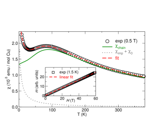
Figure 2: (Color online) Magnetic susceptibility (circles) and the fit (dashed line), see text for details. Intrinsic, i.e. Heisenberg chain (solid line) and impurity (dotted line) contributions to the fitted curve are shown. Inset: high-field magnetization curve (squares) with a linear fit (dashed line).

The extrinsic nature of the low-temperature Curie tail is supported by its suppression in magnetic field (Fig. 3). Temperature derivative of magnetic susceptibility exhibits a kink at 6 K, which is likely a signature of antiferromagnetic ordering. This issue is discussed in context of the microscopic spin model in Sec. VI.

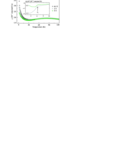
Figure 3: (Color online) Magnetic susceptibility of CaCu₂(SeO₃)₂Cl₂ measured in applied fields of 0.5 T, 2 T, and 5 T. The increase in the field leads to suppression of the low-temperature paramagnetic upturn. The inset shows the derivative of the magnetic susceptibility and a kink around 6 K, likely evidencing long-range magnetic ordering.

We also measured the magnetization curve of CaCu₂(SeO${}_{3})_{2}$Cl₂ in pulsed magnetic fields up to 60 T at a constant temperature of 1.5 K.not The linear change in the magnetization (see the inset of Fig. 2) is consistent with the proposed uniform-chain behavior, since the accessible field range is well below the saturation field ($\mu_{0}H_{s}$ = 188 T for $J$ = 133 K and $g$ = 2.11) for the parameters obtained above.

According to Sec. III, the spin chains cannot be assigned to the structural chains of the corner-sharing Cu(1)O₄ plaquettes and CuO₄Cl₂ octahedra. In Sec. V, we show that the uniform chains originate from a nontrivial superexchange pathway via SeO₃ groups.

V Microscopic model

Band structure calculations have been performed using the full-potential code fplo9.00-31.Koepernik and Eschrig (1999) For the exchange and correlation potential, the parameterization of Perdew and Wang has been chosen.Perdew and Wang (1992) For the calculations within the local density approximation (LDA), a well converged $k$-mesh of 10$\times$10$\times$12 points was used. For spin-polarized supercell local spin density approximation (LSDA)+$U$ calculations, we used $k$-meshes of 4$\times$4$\times$4 and 4$\times$4$\times$2 points. Convergence of total energy with respect to the $k$-mesh has been carefully checked.

LDA yields a valence band (Fig. 4, top) with the bandwidth of about 8 eV, typical for cuprates.Janson et al. (2007, 2009); Tsirlin et al. (2010); Janson et al. (2010) The band is clearly split into two parts: the region between $-8$ and $-5.5$ eV is dominated by Se $4p$ and O $2p$ states, while the rest of the valence band is formed by Cu, O, and Cl states. Non-zero density of states (DOS) at the Fermi level $\varepsilon_{\text{F}}$ indicates a metallic solution in contrast to the insulating behavior, expected from the green sample color. This well-known drawback of the LDA arises from a strong underestimation of correlations which are intrinsic for the $3d^{9}$ electronic configuration (Cu²⁺) and drive the system into the insulating regime.Pickett (1989)

The states relevant for magnetism are confined to the vicinity of $\varepsilon_{\text{F}}$. In most cuprates, these are the antibonding Cu $3d_{x^{2}-y^{2}}$ and O $2p_{\sigma}$ states (in the local coordinate system), typically well-separated from the rest of the valence band.Salguero et al. (2007); Janson et al. (2007, 2009); Tsirlin and Rosner (2010) However, CaCu₂(SeO${}_{3})_{2}$Cl₂ lacks a separated band complex around $\varepsilon_{\text{F}}$. This reflects the octahedral coordination for Cu(2) and makes a detailed analysis of the magnetically active orbitals necessary.

To evaluate the relevant states, we project the DOS onto a set of local orbitals. This way, we find the dominant $3d_{x^{2}-y^{2}}$ contribution to the Cu(1) DOS at $\varepsilon_{\text{F}}$ (Fig. 4, left bottom), as for almost all undoped cuprates. For the Cu(2) atom, the situation is less trivial, since the local environment of this atom implies two short Cu(2)–O bonds as well as four long (two Cu(2)–O and two Cu(2)–Cl) almost equidistant bonds, making the choice of the local coordinate system ambiguous. However, the analysis of local DOS for different situations readily yields the correct choice of the local axes and evidences that the two short Cu(2)–O and two Cu(2)–Cl bonds form a plaquette with the Cu $3d_{x^{2}-y^{2}}$ magnetically active orbital (Fig. 5). The local DOS of this orbital clearly dominates the states at $\varepsilon_{\text{F}}$ (Fig. 4, right bottom) and confirms our empirical considerations presented in Sec. III.

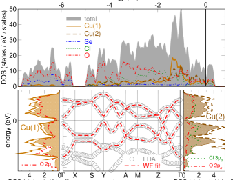
Figure 4: (Color online) Top: total (shaded) and atomic-resolved (lines) density of states (DOS) for CaCu₂(SeO${}_{3})_{2}$Cl₂. Bottom center: LDA band structure (circles) and the WF fit (dashed line). Bottom left and right: orbital-resolved density of states for Cu(1) and Cu(2). Solid $[$dashed$]$ lines denote total DOS for Cu(1) $[$Cu(2)$]$. Shaded regions show the $3d_{x^{2}-y^{2}}$ contribution. O 2p_σ (Cl 3p_σ) DOS are shown with dash-dotted (dotted) lines.

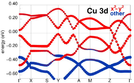
Figure 5: (Color online) Band weights for the magnetically active Cu $3d_{x^{2}-y^{2}}$ and other Cu $3d$ orbitals.

Since the magnetism of CaCu₂(SeO${}_{3})_{2}$Cl₂ is confined to Cu $3d_{x^{2}-y^{2}}$ orbitals, they can be used as a minimal basis for an effective tight-binding (TB) model. The total number of states (four) in the model corresponds to the number of magnetic Cu atoms in a unit cell: two Cu(1) and two Cu(2). To parameterize the model, we use the Wannier functions (WFs) technique, which yields numerical values for the leading hoppings $t_{i}$ (transfer integrals). This way, we obtain a perfect fit to the LDA bands (Fig. 4, bottom).

Within the effective one-orbital TB model, we find three relevant couplings (Table 4): $t_{1}$ (Figs. 6 and 7) running along Cu(1)-Cu(2) chains almost parallel to the $[201]$ direction, the short-range interchain coupling $t_{\text{ic}1}$ which connects Cu(1) atoms, as well as the long-range interchain coupling $t_{\text{ic}2}$ connecting Cu(2) atoms along $[10\bar{1}]$. The clearly dominant $t_{1}$ amounts to 139 meV, while $t_{\text{ic}1}$ and $t_{\text{ic}2}$ are found to be 47 and 30 meV, respectively. Due to the particular orientation of magnetically active orbitals, the hopping $t_{\text{nn}}$ along the “structural chains” is apparently small, does not affect the magnetic ground state, as will be shown later.

Table 4: Interatomic Cu–Cu distances ($d$, in Å), transfer integrals ($t_{i}$, in meV), as well as antiferromagnetic (AFM) and ferromagnetic (FM) contributions to the total exchange integrals ($J_{i}$, in K) for the leading couplings in CaCu₂(SeO${}_{3})_{2}$Cl₂. For notation of the paths see Fig. 7 ($J_{\text{nn}}$ stands for the nearest-neighbor coupling along the structural chains).

path	atoms	$d$	$t_{i}$	$J^{\text{AFM}}_{i}$	$J^{\text{FM}}_{i}$	$J_{i}$
$J_{\text{nn}}$	Cu(1), Cu(2)	3.84	19	4	$-$	4
$J_{\text{ic}1}$	Cu(1), Cu(1)	4.13	47	25	$-15$	10
$J_{1}$	Cu(1), Cu(2)	6.19	139	200	$-55$	145
$J_{\text{ic}2}$	Cu(2), Cu(2)	7.33	30	10	$-$	10

Figure 6: (Color online) Wannier functions marking the $J_{1}$ superexchange path. Cu(1)O₄ (left) and Cu(2)O₂Cl₂ (right) plaquettes are filled. The SeO₃ pyramid is visualized by Se–O bonds (lines). The projection is the same as in Fig. 1 (left).

To restore the insulating ground state, we map our TB model onto a Hubbard model with an effective on-site Coulomb repulsion $U_{\text{eff}}$. Since the strongly correlated limit ($U_{\text{eff}}$ ${\gg}$ $t_{i}$) and the half-filling are well-justified for undoped cuprates, the low-energy (magnetic) excitations of the Hubbard model can be well described by a Heisenberg model. Within the second-order perturbation theory, AFM exchange couplings are expressed as $J^{\text{AFM}}_{i}$ = $4t^{2}_{i}/U_{\text{eff}}$. Adopting a typical value $U_{\text{eff}}$ = 4.5 eV,Janson et al. (2009, 2007); Tsirlin and Rosner (2010) we obtain $J^{\text{AFM}}_{1}$ = 200 K, $J^{\text{AFM}}_{\text{ic}1}$ = 25 K and $J^{\text{AFM}}_{\text{ic}2}$ = 10 K.

The one-orbital approach yields only the AFM part $J^{\text{AFM}}_{i}$ of the total exchange $J_{i}$. However, particular geometrical configurations (Cu–O–Cu angle close to 90^∘, edge-sharing of CuO₄ plaquettes etc.) often lead to sizable ferromagnetic (FM) contributions to the total exchange, which can even outgrow $J^{\text{AFM}}_{i}$, resulting in a FM (negative) $J_{i}$. Based on structural considerations only, an appreciable FM contribution might be expected for the short-range coupling $J_{\text{ic}1}$ and the nearest-neighbor coupling $J_{\text{nn}}$, whereas $J_{1}$ and $J_{\text{ic}2}$ are rather long-range, and their FM contributions should be small. To challenge this conjecture, we perform supercell LSDA+$U$ calculations. This method gives access to the total exchange $J_{i}$, being the sum of the AFM and FM contributions, $J^{\text{AFM}}_{i}$ and $J^{\text{FM}}_{i}$, respectively. Combining the LSDA+$U$ results with $J^{\text{AFM}}_{i}$ estimates from the model approach described above, the FM contributions $J^{\text{FM}}_{i}$ can be evaluated.

Recent thorough studies on low-dimensional cuprates give evidence that quantitative magnetic models based on the results of LSDA+$U$ calculations are, in addition to the dependence on the Coulomb repulsion $U_{d}$, also dependent on the double-counting correction (DCC) scheme.Tsirlin et al. (2010); Janson et al. (2010) The influence of these two parameters is particularly large for systems with sizable $J^{\text{FM}}_{i}$. Yet, for cuprates with structurally isolated plaquettes, as in the case of CaCu₂(SeO${}_{3})_{2}$Cl₂, the around-mean-field (AMF) DCC with the $U_{d}$ value 6.5 $\pm$ 0.5 eV typically yields accurate ($\pm 10\%$) estimates for the leading couplings. Adopting the AMF DCC and $U_{d}$ = 6.5 eV, we obtain $J_{1}$ = 145 K, in excellent agreement with the experimental $J$ $\simeq$ 133 K from the fit to the magnetic susceptibility. In accordance with our expectations, the long-range interchain coupling $J_{\text{ic}2}$ has a tiny FM contribution only, while for the short-range coupling $J_{\text{ic}1}$ the FM contribution reaches $J^{\text{FM}}_{\text{ic}1}$ = $-$15 K (see Table 4). At first glance, the rather large $J^{\text{FM}}_{1}\sim-55$ K may look surprising. However, in the related quasi-1D system CuSe₂O₅, a similar intrachain coupling runs via two corner-sharing SeO₃ pyramids and the FM contribution $J^{\text{FM}}_{1}$ to this coupling amounts to even $-$100 K.Janson et al. (2009) Therefore, such high FM contributions are likely intrinsic to the superexchange realized via SeO₃ pyramids. Understanding the underlying mechanism of this complex superexchange deserves a separate study and lies beyond the scope of the present investigation. Presently, we note that the superexchange results from the overlap of oxygen orbitals, while Se states have only a minor contribution to the WFs.

The last remark concerns the short-range coupling between the nearest-neighbor Cu(1) and Cu(2) atoms that form the structural chains. The WFs analysis yielded a negligible $t$ associated with this coupling path. Still, the respective interatomic distance (3.84 Å) is relatively small, which could give rise to a FM coupling. Therefore, we evaluated the total exchange $J_{\text{nn}}$ using the LSDA+$U$ calculations. The resulting exchange of 4 K is in excellent agreement with the TB estimate (4 K), evidencing a negligible FM contribution and justifying our restriction to the three couplings $J_{1}$, $J_{\text{ic}1}$, and $J_{\text{ic}2}$ for a minimum model.

VI Discussion and summary

The spin model of CaCu₂(SeO${}_{3})_{2}$Cl₂ is depicted in Fig. 7. Its main element are Cu(1)–Cu(2) chains running almost parallel to the $[201]$ direction, which is different from the structural chains. The spin-$\frac{1}{2}$ chains are coupled by two inequivalent exchange interactions: $J_{\text{ic}1}$ is short-range and links the Cu(1) atoms of the two neighboring chains, while the long-range $J_{\text{ic}2}$ bridges the Cu(2) atoms of the fourth-neighbor chains. Another difference between $J_{\text{ic}1}$ and $J_{\text{ic}2}$ is that the former is responsible for a 3D coupling $[$connects Cu(1) atoms belonging to different layers, see Fig. 7$]$, whereas the latter is confined to the $ac$ plane. Either of inter-chain couplings alone, $J_{\text{ic}1}$ or $J_{\text{ic}2}$, leads to a 3D or 2D non-frustrated model, respectively. However, the combination of the two inter-chain couplings gives rise to magnetic frustration, evidenced by an odd number of AFM bonds along the closed, hourglass-shaped loop shown in Fig. 7.

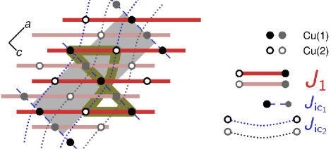
Figure 7: (Color online) Spin model for CaCu₂(SeO${}_{3})_{2}$Cl₂. Filled and empty circles show the Cu(1) and Cu(2) positions. Bold lines and circles denote couplings (see legend for notation; the same notation applies for Table 4) in the front plane, whereas gray circles and shaded lines correspond to the atoms lying in the back plane. The planes are connected by $J_{\text{ic}1}$ couplings only. A closed loop (bold line) having an odd number of AFM couplings indicates that the spin model is frustrated. The unit cell is depicted by the gray rectangle.

In general, most of the quasi-one-dimensional cuprates order AFM at low temperatures, while strong quantum fluctuations drastically reduce the value of the ordered moment compared to the classical value of 1 $\mu_{\text{B}}$.*[See; e.g.][andreferencestherein.]sr2cuo3 The AFM transition temperature can vary in a wide range, since it depends not only on the leading intrachain coupling $J_{1}$, but also on the absolute values and the topology of the interchain couplings. To emphasize the huge impact of the interchain coupling regime onto the transition temperature, we mention here two quasi-one-dimensional systems with similar intrachain coupling $J_{1}$ of 150–200 K, but different interchain coupling regimes: a frustrated interchain coupling in Sr₂Cu(PO₄)₂ leads to a very low ordering temperature of 85 mK ($T_{N}/J$ = 4.5$\times$10^-4) (Ref. Belik et al., 2005) despite an interchain coupling of 3 K.Johannes et al. (2006) On the contrary, a sizable and non-frustrated interchain coupling $J_{\text{ic}}$ $\sim$ 20 K in CuSe₂O₅ results in a long-range AFM ordering at rather high $T_{N}$ = 17 K ($T_{N}/J$ = 0.1).Janson et al. (2009)

Since CaCu₂(SeO${}_{3})_{2}$Cl₂ exhibits a similar energy scale ($J_{1}$ $\sim$ 133 K), it is natural to compare this compound to the aforementioned systems. The major difference here is the presence of two types of interchain couplings, $J_{\text{ic}1}$ and $J_{\text{ic}2}$, which form a 3D spin model, in contrast to Sr₂Cu(PO₄)₂ and CuSe₂O₅, where the leading interchain couplings are confined to 2D, while the coupling along the third direction $J_{\perp}$ is substantially smaller. This argument favors higher $T_{N}$ in CaCu₂(SeO${}_{3})_{2}$Cl₂. On the other hand, the interchain couplings in CaCu₂(SeO${}_{3})_{2}$Cl₂ are frustrated, which certainly inhibits the magnetic ordering and can considerably lower the $T_{N}$. We expect the combination of the 3D coupling regime and the frustration to result in a moderate $T_{N}$ of CaCu₂(SeO${}_{3})_{2}$Cl₂, comparable to that of CuSe₂O₅. Indeed, the kink of magnetic susceptibility at 6 K in Fig. 3 fits well to the energy scale of the anticipated long-range ordering in CaCu₂(SeO${}_{3})_{2}$Cl₂ (compare to $T_{N}$ = 17 K in CuSe₂O₅ with non-frustrated interchain couplings).

In general, magnetic specific heat $C_{p}^{\text{magn}}$ data provide an independent estimate for the leading exchange coupling and are sensitive to the long-range magnetic ordering. However, the measured specific heat contains, apart from $C_{p}^{\text{magn}}$, also a phonon contribution. The energy scale of magnetic interactions in CaCu₂(SeO${}_{3})_{2}$Cl₂ gives rise to a maximum in $C_{p}^{\text{magn}}(T)$ at rather high $T$ $\approx$ (0.48 $J$) = 64 K (Eq. 39 in Ref. Johnston et al., 2000). At this temperature, the phonon specific heat strongly dominates over $C_{p}^{\text{magn}}$, impeding an accurate disentanglement of magnetic and phonon contributions. Moreover, the large value of $J$ leads to only a small amount of magnetic entropy, which could be released at the transition temperature. Thus, the resulting magnetic specific heat anomaly would be rather small.*[See; e.g.][]HC_AgCuVO4 Therefore, considering large quantum fluctuations that substantially lower the ordered magnetic moment,Kojima et al. (1997) the method of choice are muon spin resonance ($\mu$SR) experiments that should be carried out in future to verify magnetic ordering in CaCu₂(SeO${}_{3})_{2}$Cl₂. For instance, long-range magnetic ordering in the square-lattice compounds Cu(Pz)₂(ClO₄)₂ and $[$Cu(Pz)₂(HF₂)$]$BF₄ was only revealed by $\mu$SR, while the heat capacity data lack any signatures of transition anomalies.Lancaster et al. (2007)

Magnetic frustration is one of the leading mechanisms that give rise to complex magnetic structures. It is therefore interesting to address the nature of the anticipated magnetically ordered ground state of CaCu₂(SeO${}_{3})_{2}$Cl₂. First, we consider the low-energy sector of a classical Heisenberg model on finite lattices of 16 coupled chains. For each chain, we impose a condition of the ideal antiferromagnetic arrangement of the neighboring spins. To keep the problem computationally feasible, we first restrict ourselves to collinear spin arrangements. The magnetic ground state is evalauted as a state with minimal energy. Adopting the ratios of the leading exchange couplings from our LSDA+$U$ calculations (Table 4, last column), we arrive at an AFM ground state, with the magnetic unit cell doubled along $a$ and quadrupled along $c$ with respect to the crystallographic unit cell, i.e. the propagation vector is $(\frac{1}{2},0,\frac{1}{4})$. To understand the particular way the frustration is lifted, we analyse which couplings are satisfied, by considering the products $-$4$[\vec{S}_{i}\cdot\vec{S}_{j}](J_{ij}/|J_{ij}|)$ for all $(i,j)$ spin pairs in a unit cell. For collinear configurations, such product amounts either to 1 (a satisfied coupling) or to $-1$ (an unsatisfied coupling). For a certain type of exchange coupling, the sum of such products can be divided by the total number of couplings of this type in the unit cell (note the multiplicities different from 1). This way, we can estimate the fraction of satisfied couplings. Such analysis yields that 100 % of $J_{1}$ and $J_{\text{ic2}}$, but only 75 % of $J_{\text{ic1}}$ couplings are satisfied in the proposed $(\frac{1}{2},0,\frac{1}{4})$ ground state.

Taking into account the restriction to collinear states, it is worth to address the stability of this ground state using alternative techniques. Thus, we use a classical Monte-Carlo code from the alps simulations packageAlbuquerque et al. (2007) and calculate diagonal spin correlations ${\langle}S^{z}_{i}S^{z}_{j}\rangle$, where $i$ and $j$ are spins coupled by a particular magnetic exchange. This way, we obtain $-$0.24452(1), $-$0.16716(1) and $-$0.23056(3) for the $J_{1}$, $J_{\text{ic}1}$ and $J_{\text{ic}2}$ couplings, respectively. These numbers should be compared to ${\langle}S^{z}_{i}S^{z}_{j}\rangle$ = $-$0.25 for a perfect antiferromagnetic arrangement. Despite the small deviations from this ideal number, the spins coupled by $J_{1}$ and $J_{\text{ic2}}$ can be regarded as antiferromagnetically arranged, corroborating our classical energy minimization result. On the contrary, the value for $J_{\text{ic1}}$ is substantially smaller, yielding the average angle of $\arccos{(0.16716/S^{2})}$ $\approx$ 48 ^∘ between the respective spins. The resulting angle is very close to $\pi/4$, hence spins in the fourth-neighbor chains are almost antiparallel to each other (the angle amounts to $\pi$). This is in accord with the almost antiparallel arrangement of spins coupled by $J_{\text{ic2}}$ (coupling between the fourth-neighbor chains).

In the classical model, the exotic regime of frustrated interchain couplings leads to a rather complex magnetic ordering in CaCu₂(SeO${}_{3})_{2}$Cl₂: the classical energy minimization yields the collinear $(\frac{1}{2},0,\frac{1}{4})$ state, while the classical Monte Carlo simulations are in favor of a non-collinear magnetic ground state. These two ground states differ only by the mutual arrangement of spins coupled by $J_{\text{ic1}}$.

Since for quasi-one-dimensional systems quantum fluctuations are crucial, the respective quantum model should be addressed. However, the study of a magnetic ordering for a three-dimensional frustrated quantum magnet is a challenging task, since standard methods, such as exact diagonalization, quantum Monte-Carlo, and the density matrix renormalization group technique, are either not applicable or do not account for the thermodynamic limit. Moreover, CaCu₂(SeO${}_{3})_{2}$Cl₂ features a non-negligible magnetic impurity contribution, as evidenced by the low-temperature upturn in $\chi(T)$ (Fig. 2). At low temperatures, these impurities can give rise to strong internal fields,[Similareffectwasrecentlydiscussedfortheanisotropictriangularlatticemodelintheone-dimensionallimit; see][]HC_Cs2CuCl4_theory and possibly affect the ground state. Therefore, the magnetic ordering in CaCu₂(SeO${}_{3})_{2}$Cl₂ deserves additional investigation using alternative techniques, both from the experimental as well as the theoretical side.

In contrast to well-known uniform-chain systems, CaCu₂(SeO${}_{3})_{2}$Cl₂ shows a complex crystal structure with two Cu positions revealing an apparently different local environment. Our DFT calculations evaluate the $3d_{x^{2}-y^{2}}$ magnetically active orbitals lying within the Cu(1)O₄ and Cu(2)O₂Cl₂ plaquettes. Although the Cu(2)–O3 bond lengths are similar to those of Cu(2)–Cl bonds, the symmetry of the magnetic orbitals renders the nearest-neighbor superexchange $J_{\text{nn}}$ path (along Cu(2)–O3 bonds) essentially inactive (Table 4). The spin chains run in a different direction which is dictated by the orbital state of Cu and by the suitable overlap of the ligand orbitals in the SeO₃ groups. This nontrivial situation is very typical for spin-1/2 systems where spin lattices are essentially decoupled from the low-dimensional features of the crystal structure: recall, for example, (CuCl)LaNb₂O₇,Tsirlin and Rosner (2010) BiCu₂PO₆,Tsirlin et al. (2010) Cu₂(PO${}_{3})_{2}$CH₂,Schmitt et al. (2010) and CuTe₂O₅.Ushakov and Streltsov (2009)

Although the intricate regime of the interchain couplings in CaCu₂(SeO${}_{3})_{2}$Cl₂ complicates theoretical studies, the nontrivial structural organization of this compound also has an important advantage. The Cl and Br atoms are known to be easily substitutable owing to their similar chemical nature. The substitution is commonly used to create bond randomness and to access the exotic behavior of partially disordered spin systems.[Forexample:][]manaka2008 If the Cl atoms take part in the superexchange, the chemical substitution inevitably changes the geometry of the superexchange pathways, and immediately leads to dramatic changes in the spin system. In CaCu₂(SeO${}_{3})_{2}$Cl₂, the Cl atoms lie away from the leading superexchange pathway (Fig. 6), and a moderate alteration of the magnetism should be expected. Partial Cl/Br substitution will basically modify the relevant microscopic parameters (such as the crystal-field splitting) without changing the superexchange geometry.

In summary, we have investigated the crystal structure, electronic structure, and magnetic behavior of CaCu₂(SeO${}_{3})_{2}$Cl₂. The compound comprises two Cu sites with essentially different local environment, but the same magnetically active orbital of local $x^{2}$ $-$ $y^{2}$ symmetry. A peculiar arrangement of magnetic plaquettes makes CaCu₂(SeO${}_{3})_{2}$Cl₂ a good realization of the spin-$\frac{1}{2}$ antiferromagnetic Heisenberg chain model with an intrachain exchange coupling of $\sim$133 K and frustrated interchain couplings realized via two inequivalent superexchange paths. A kink in the magnetic susceptibility at 6 K hints at long-range magnetic ordering, which is subject to future experimental verification. The good potential for a partial substitution of Cl by Br atoms allows to look at the material from a different point of view. In particular, Cl atoms located close to but not directly on the leading superexchange path make CaCu₂(SeO${}_{3})_{2}$Cl₂ a promising model system to study the bond-randomness effects — like glass formation — in low-dimensional magnets.