To synchronize or not to synchronize, that is the question: finite-size scaling and fluctuation effects in the Kuramoto model

Abstract

The entrainment transition of coupled random frequency oscillators presents a long-standing problem in nonlinear physics. The onset of entrainment in populations of large but finite size exhibits strong sensitivity to fluctuations in the oscillator density at the synchronizing frequency. This is the source for the unusual values assumed by the correlation size exponent $\nu^{\prime}$. Locally coupled oscillators on a $d$-dimensional lattice exhibit two types of frequency entrainment: symmetry-breaking at $d>4$, and aggregation of compact synchronized domains in three and four dimensions. Various critical properties of the transition are well captured by finite-size scaling relations with simple yet unconventional exponent values.

1 Introduction

Mathematical modeling of coherent oscillation in a large population of autonomous units has a long and interesting history, as discussed in several monographs[1, 2] and recent reviews[3, 4, 5]. One particular paradigm is the Kuramoto model of coupled random frequency oscillators[2]. In terms of the phase variables $\phi_{j},j=1,\ldots,N$, the dynamical equations take the form,

$${d\phi_{j}\over dt}=\omega_{j}-K\Delta\sin(\phi_{j}-\theta).$$ (1)

Here $K$ is the coupling strength among the oscillators, and $\Delta(>0)$ and $\theta$ are the amplitude and phase of the mean instantaneous phase factor,

$$\Delta e^{i\theta}\equiv N^{-1}\sum_{j=1}^{N}e^{i\phi_{j}},$$ (2)

which is also known as the order parameter for entrainment. The intrinsic frequencies $\omega_{j}$ are drawn from a distribution $g(\omega)$. In this paper we shall focus on the case where $g(\omega)$ is a gaussian function centered at $\omega_{\rm max}=0$ with unit variance.

In the classic work by Kuramoto[2], existence of an entrained state is established by considering solutions to (1) at a constant $\Delta$. Under this assumption, Eq. (1) is easily integrated. After an initial transient, oscillators with $|\omega_{j}|<K\Delta$ each reaches a fixed angle and together form the entrained group, while those with $|\omega_{j}|>K\Delta$ go into periodic motion at modified frequencies $\tilde{\omega}_{j}=\sqrt{\omega_{j}^{2}-(K\Delta)^{2}}$. In the limit $N\rightarrow\infty$, only the entrained population contributes to the sum (2). The resulting self-consistent condition

$$\Delta=\int_{-K\Delta}^{K\Delta}d\omega g(\omega)\sqrt{1-(\omega/K\Delta)^{2}}$$ (3)

has a nontrival solution $\Delta>0$ when $K>K_{c}=2/\pi g(0)$. Thus entrainment requires the product $Kg(0)$ to exceed a threshold value. On the supercritical side, $\Delta(K)\sim(K-K_{c})^{\beta}$ with the usual mean-field exponent $\beta=1/2$.

While the above predictions agree well with numerical solutions of the globally coupled Kuramoto model, there are several unresolved issues regarding the stability of the mean-field solution, as discussed elegantly in Ref. [3]. From a physicist’s point of view, one would like to understand how temporal fluctuations of $\Delta(t)$, which are present when the sum (2) contains only a finite number of terms, affect the behavior predicted by the mean-field treatment. When the oscillator frequencies $\omega_{j}$ are drawn independently from the distribution $g(\omega)$, sample-to-sample fluctuations in the time averaged $\Delta$ need to be considered as well. These effects culminate at $K=K_{c}$ where the size of the entrained group grows sub-linearly with the system size $N$.

Daido developed a perturbation theory[6] to calculate the susceptibility defined by,

$$\chi\equiv N\bigl{(}\overline{\Delta^{2}}-\overline{\Delta}^{2}\bigr{)}$$ (4)

Here the overline bar denotes time average. His calculation yielded a power-law divergence of $\chi$ at $K_{c}$, but the exponent $\gamma$ differs on the two sides of the transition: $\gamma=\gamma_{-}=1$ on the subcritical side and $\gamma=\gamma_{+}=1/4$ on the supercritical side. Daido has further suggested a finite-size scaling form based on his own numerical studies,

$$\chi=|k|^{-\gamma_{\pm}}\Phi(kN^{1/\nu_{\pm}^{\prime}}).$$ (5)

Here $k=(K-K_{c})/K_{c}$ is the distance to the transition, $\nu_{-}^{\prime}=2$ and $\nu_{+}^{\prime}=1/2$. These exponent values unfortunately do not agree with later numerical work[7].

Equations (1) have been adapted to describe synchronization phenomena in finite dimensions with local oscillator coupling[8],

$${d\phi_{j}\over dt}=\omega_{j}-K\sum_{l\in\Lambda_{j}}\sin(\phi_{j}-\phi_{l}).$$ (6)

Here $\Lambda_{j}$ denotes the set of the nearest neighbor sites of $j$ on a $d$-dimensional hypercubic lattice. Arguments have been presented to show that, as the linear system size $L\rightarrow\infty$, global entrainment is not possible when $d<2$[8]. Analytical and numerical studies of the model in three to six dimensions by Hong, Chatè, Park and Tang (HCPT)[9] have established the following. For $d>4$, the entrainment transition is of the symmetry-breaking type with exponents indicative of a mean-field behavior. At $d=3$ and 4, on the other hand, global entrainment is reached through aggregation of locally synchronized domains as the coupling strength $K$ increases beyond a critical value $K_{c}$. Although the aggregation process is continuous and can be associated with a length scale $\xi$ that diverges at $K_{c}$, the fraction of entrained oscillators may undergo a discontinuous jump at $K_{c}$ in the limit $L\rightarrow\infty$.

Below we shall give an overview of our current knowledge on the finite-size scaling properties in the all-to-all coupled Kuramoto model and discuss some fine differences between this case and the Kuramoto model on a random graph. We shall argue that the latter provides the correct mean-field description of the entrainment transition at $d>4$. Key features of the entrainment process in three and four dimensions are also discussed. However, no attempt is made to review the vast amount of related work in the literature. Fortunately, this role is partially fulfilled by several recent articles cited above.

2 Finite-size scaling in the globally coupled model

2.1 Anomalous behavior due to quenched frequency fluctuations

In typical numerical studies of (1), the frequencies $\omega_{j}$ are drawn independently from the distribution $g(\omega)$. HCPT have shown that, in this case, $\nu^{\prime}=5/2$ on either side of the transition. Since the argument is quite straightforward and relevant for the discussion of synchronization on complex networks and in finite dimensions, we reproduce it below.

Still assuming $\Delta$ in (1) to be time-independent and restricting the sum in (2) to the entrained oscillators in a finite population, Eq. (3) is replaced by

$$\Delta=\Psi(\Delta)\equiv{1\over N}\sum_{j,|\omega_{j}|<K\Delta}\sqrt{1-\Bigl{(}{\omega_{j}\over K\Delta}\Bigr{)}^{2}}.$$ (7)

Since the actual values of the $\omega_{j}$’s vary from sample to sample, the sum $\Psi$ has a “quenched” fluctuation $\delta\Psi\equiv\Psi-\langle\Psi\rangle\propto N_{s}^{1/2}/N$, where $N_{s}$ is the number of oscillators in the frequency interval $(-K\Delta,K\Delta)$. Here $\langle\cdot\rangle$ denotes average over different realizations of the random frequencies. Close to the transition, an expansion of Eq. (7) at small $\Delta$ yields,

$$\Delta=(K/K_{c})\Delta-c(K\Delta)^{3}+\delta\Psi,$$ (8)

where $c=-\pi g^{\prime\prime}(0)/16$. Mathematically, the variance of $\delta\Psi$ can be computed from (7) for independently drawn frequencies: $\langle(\delta\Psi)^{2}\rangle=4g(0)K\Delta/3N+O(\Delta^{2}/N)$. Thus solution to (8) takes the scaling form,

$$\Delta(K,N)=N^{-1/5}f(kN^{2/5}).$$ (9)

The scaling function $f(x)$ is sample-dependent and satisfies the equation,

$$xf-cK_{c}^{3}f^{3}+(8/3\pi)^{1/2}\epsilon f^{1/2}=0.$$ (10)

Here $\epsilon\equiv\delta\Psi/\langle(\delta\Psi)^{2}\rangle^{1/2}$ is a gaussian random variable with zero mean and unit variance.

Equation (9) suggests $\nu^{\prime}=5/2$ as seen in numerical experiments. Its origin lies in the fluctuations in the oscillator density at the peak frequency $\omega_{\rm max}$ of $g(\omega)$. This effect produces a sample-dependent shift $\delta K_{c}\sim N^{-2/5}$ of the entrainment threshold. At the nominal threshold $K=K_{c}$, $\Delta_{0}\sim\delta K_{c}^{\beta}\sim N^{-1/5}$. In other words, the number of entrained oscillators right at $K=K_{c}$ scales as $N^{4/5}$. (Note that, when the term $\epsilon$ in (10) is negative, there is only the trivial solution $f=0$ at $x=0$. For these samples, the entrained population size is much smaller than $N^{4/5}$.) Numerical simulations of (10) produced values of $\langle\Delta^{2}\rangle$ in quantitative agreement with that of the Kuramoto model for $K>K_{c}$[9].

2.2 Dynamic fluctuations in the subcritical region

For $K<K_{c}$, oscillators essentially run with their intrinsic frequencies. If the phase factors in the sum (2) were all statistically independent from each other, one would have $\overline{\Delta}^{2}=1/N$ and hence $\chi=1$. The perturbative calculation by Daido[6] yielded the following expression for $K$ close to $K_{c}$:

$$\chi={A\over K_{c}-K}+D.$$ (11)

Here $A=4/K_{c}$ for the gaussian $g(\omega)$, and $D$ is a numerical constant which can also be evaluated, though the calculation is rather tedious. Equation (11) was rederived recent by Hildebrand et al. using a different approach[10].

Numerical results by Hong et al.[11] are in good agreement with (11) when the system size $N>N_{c}\sim|K-K_{c}|^{-5/2}$. At smaller values of $N$, a sample-dependent behavior is seen, so the result depends on the averaging procedure. For example, the data for $\chi$ calculated from (4) for a given sample and then averaged over many samples obey the scaling $\langle\chi\rangle\simeq|k|^{-1}\Psi(kN^{2/5})$. This implies that, in the critical region $|k|<N^{-2/5}$, dynamic fluctuations of $\Delta$ have an amplitude $\delta\Delta_{\rm dyn}\sim N^{-3/10}$, which is weaker than the sample to sample fluctuation $\Delta_{0}\sim N^{-1/5}$. Due to this difference, the hyperscaling relation $\nu^{\prime}=2\beta+\gamma$ is violated. At present, there is no analytic theory that explains these numerical findings.

2.3 Finite-size scaling in the “pure” case

The oscillator density fluctuations on the frequency axis responsible for the anomalous $\nu^{\prime}=5/2$ can be eliminated when the frequency $\omega_{j}$ of the $j$’th oscillator is chosen according to the formula

$${j-0.5\over N}=\int_{-\infty}^{\omega_{j}}g(\omega)d\omega.$$ (12)

The intrinsic frequencies of the oscillators in this case are nearly uniformly spaced locally on the axis. In analogy with the discussion of disordered systems, we call this situation the “pure” case.

Numerical simulations of the Kuramoto model with frequencies given by (12) produced exactly the same $\Delta(K)$ function in the large size limit as the “disordered” case. On the other hand, measurement of fluctuations of $\Delta(t)$ yielded $\gamma_{\pm}=1/4$ and $\nu_{\pm}^{\prime}=5/4$ which are very different from the disordered case[11]. It thus appears that the subcritical behavior (11) requires extra assumptions which are not fulfilled in the pure case.

2.4 Entrainment transition on complex networks

The entrainment transition of the Kuramoto model has been studied on complex networks by several groups[5]. Here the dynamical equations are given by (6), with $\Lambda_{j}$ denoting the set of nodes connected to node $j$ on the network. In the case of scale-free networks where the degree $k$ of nodes satisfies a power-law distribution $P(k)\sim k^{-\alpha}$, both numerical and analytical studies show that the exponent $\beta=1/2$ for $\alpha\geq 5$, but increases sharply as $\beta=1/(\alpha-3)$ for $3<\alpha<5$[12]. The size of the critical region where finite-size effects become significant, as described by the exponent $\nu^{\prime}$, also broadens in the latter case. These two effects combine to give a broadened transition when the local connectivity of the network assumes a broad distribution.

Interestingly, for $\alpha>5$, and on the random graph with a fixed degree, the finite-size scaling form (5) is found to hold across the transition, with the exponents given by $\gamma_{\pm}=3/2$ and $\nu_{\pm}^{\prime}=5/2$[13]. This is in contrast to the behavior of the Kuramoto model with all-to-all coupling. To better illustrate the difference, let us examine the distribution of the mean phase velocity $v_{j}=\overline{d\phi_{j}/dt}$ of oscillators in the neighborhood of the transition. Figure 1(a) shows a comparison of the cumulative distributions obtained from the all-to-all coupling case and on a random graph at $k=6$. Both systems are in the critical region of their respective entrainment transitions. Entrained oscillators have the same phase velocity $v_{\rm syn}\simeq 0$ as indicated by the vertical jumps of the curves. Distinct behavior is seen right above and below $v_{\rm syn}$ in the two cases. For all-to-all coupling, the curve is nearly flat, suggesting a vanishing density of oscillators in the neighborhood of $v_{\rm syn}$. Thus the entrained population is well-separated from the running oscillators. On the random graph, the vertical jump joins smoothly with the detrained regions. The rise at small $|v|$ can be fitted to a $|v|^{1/2}$-law. Consequently, the oscillator density near $v_{\rm syn}$ diverges as $|v|^{-1/2}$. The boundary between the entrained and running populations is much less well-defined in this case.

The difference in the density of oscillators near the entrainment frequency can be appreciated from the following consideration. For all-to-all coupling, the fluctuation effect on a given oscillator is due to temporal variations in the system-averaged order parameter $\Delta$ which vanishes in the large size limit. In addition, from the scaling $\Delta_{\rm dyn}\sim N^{-3/10}$ and $\Delta_{0}\sim N^{-1/5}$ mentioned above, $\Delta$ can be regarded as a constant in the first approximation even in the critical region. The mean phase velocity of oscillators then essentially follows the behavior predicted by Kuramoto’s mean-field analysis, which is what the black curve in Fig. 1(a) suggests. In contrast, on the random graph, each oscillator is coupled to a small number of other oscillators. Hence the fluctuation effect has a finite strength and does not decrease significantly in the infinite size limit. Oscillators with the “right environment” first become entrained, but due to the presence of fluctuations, they undergo diffusive phase motion in a weak ordering field $\Delta$, punctuated with phase slips. This diffusive background is present even on the entrained side.

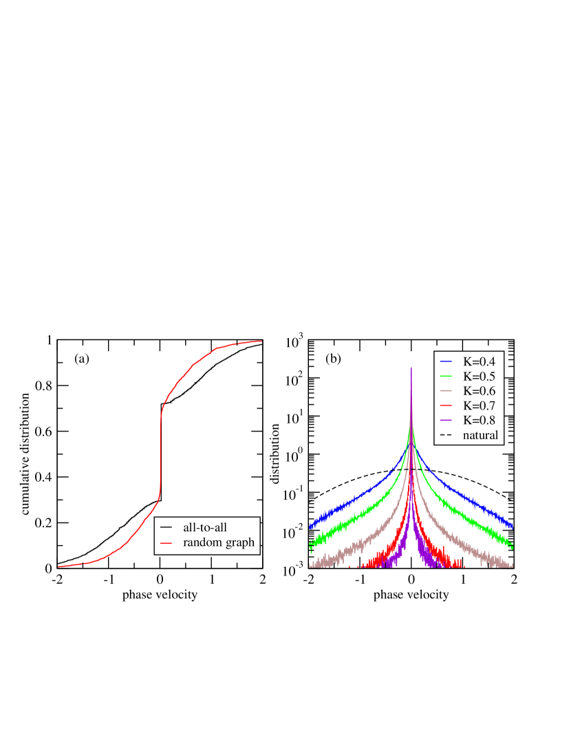
Figure 1: (Color online) (a) The cumulative distribution of the phase velocity at criticality for all-to-all (black, $K=\sqrt{8/\pi}$) and random-graph (red, $K=0.38$, degree = 6) couplings. Here $N=3200$ in both cases. (b) The phase velocity distribution in a given sample in three dimensions at different coupling strength $K$. Here $N=128^{3}$ and $K_{c}\simeq 0.7$. Dashed line indicates the frequency distribution at $K=0$.

3 The Kuramoto model in finite dimensions

The “quenched” random frequencies in (6) introduce a static phase deformation $\phi_{j}^{(0)}$ whose spatial structure has been argued to be responsible for the different types of entrainment behavior in finite dimensions[9]. Salient features of this static phase field are captured by a linear analysis carried out by Sakaguchi et al.[8] and by Hong et al.[14] The resulting dynamic equations, which reduces to the “quenched Edwards-Wilkinson equation”[15] in the continuum limit, exhibit a diffusive relaxation towards a “fully entrained” state with vanishing phase velocity for all oscillators. As the linear system size $L\rightarrow\infty$, fluctuations of $\phi_{j}^{(0)}$ remain bounded when the system dimension $d>4$, but diverge when $d\leq 4$. In addition, the gradient of $\phi_{j}^{(0)}$ diverges when $d\leq 2$.

HCPT proposed a plausible scenario for the entrainment transition based on the linear analysis. The linear approximation is justified at sufficiently large $K$ and above the lower critical dimension $d_{l}=2$, where the run-away oscillators are absent. (We assume here that the intrinsic frequencies are bounded.) As the coupling strength $K$ decreases, more and more oscillators break away from entrainment. The question is whether the remaining oscillators can stay phase-locked as their fraction in the population diminishes. For $d>4$, the entrained state has bounded phase fluctuations and hence breaks the phase symmetry $\phi\rightarrow\phi+c$. In this case, $\Delta$ as defined by Eq. (2) can still be used as a global order parameter and acts as a spontaneous ordering field on the oscillators as in the globally coupled case. On the other hand, for $d\leq 4$, the phase symmetry is not broken. Therefore phase-locking need to be maintained via a percolative network of entrained oscillators in space. The latter requires a finite density of these oscillators given the random assignment of the oscillator frequencies. The entrainment transition, when viewed in terms of the fraction of entrained oscillators in the system, is expected to be discontinuous.

The above picture is largely confirmed by extensive simulations carried out by HCPT in three to six dimensions which also yielded additional details of the entrainment transition[9]. In five and six dimensions, the distribution of the mean phase velocity shows essentially the same behavior as the Kuramoto model on a random graph as depicted in Fig. 1(a). On the other hand, a very different distribution of phase velocities is obtained in three and four dimensions. Figure 1(b) presents an example from a $N=128^{3}$ system in three dimensions. Significant narrowing of the distribution takes place at $K$ values well below the threshold $K_{c}\simeq 0.7$ at this size. The wings of the distribution can be fitted to a power-law $P(v)\sim|v|^{-2}$. The data is consistent with the picture that, below $K_{c}$, entrainment takes place locally through the formation of entrained clusters. The size of the clusters grow as $K$ increases, reaching the system size at $K_{c}$. The increase of the entrainment threshold with the system size, as observed in simulations, can be taken as further confirmation of this picture[9].

HCPT also examined various singular behavior of the system at the entrainment transition with the help of finite-size scaling analysis. For $d>4$, $\Delta$ as defined by Eq. (2) is a suitable order parameter. For $d=3$ and 4, static phase fluctuations in a sufficiently large system render $\Delta$ vanish even on the entrained side. Instead, the Edwards-Anderson order parameter

$$\Delta_{\rm EA}=\lim_{t-t_{0}\rightarrow\infty}{1\over N}\Bigl{|}\sum_{j}e^{i[\phi_{j}(t)-\phi_{j}(t_{0})]}\Bigr{|}$$ (13)

was found to be appropriate. Numerical results for a range of system sizes are in good agreement with the finite-size scaling

$$\langle\Delta^{2}\rangle,\langle\Delta^{2}_{\rm EA}\rangle=L^{-2\beta/\nu}\tilde{\Phi}(kL^{1/\nu}).$$ (14)

The exponent values extracted from the simulation data can be expressed as,

$$d \leq 4:\qquad\beta=0,\quad\nu=2/(d-2);$$

$$d > 4:\qquad\beta=1/2,\quad\nu=5/(2d),\quad\nu^{\prime}\equiv d\nu=5/2.$$ (15)

Note that in three and four dimensions, $\beta=0$ is consistent with a jump in the fraction of entrained oscillators at the transition.

4 Conclusions and outlook

Numerical investigations of the Kuramoto model with all-to-all coupling, on scale-free networks and random graphs, and on finite dimensional lattices, revealed a wealth of behavior at the onset of global entrainment. The usual finite-size scaling approach has been shown to be successful in capturing the key critical properties of these systems, including fluctuation effects and the size of the entrained population at the transition. Development of phenomenological arguments based on various approximations enhanced our understanding of the entrainment process. However, a full analytic theory of fluctuations is still lacking, even in the case of the Kuramoto model with all-to-all coupling.

The original Kuramoto model (1) has a small parameter $\Delta$ in the neighborhood of the transition which can be employed for systematic expansions. However, such a treatment need to be handled with care when considering oscillators with $\omega_{j}$’s comparable to $\Delta$. These oscillators are in fact the ones that become entrained first and contribute significantly to $\Delta$. The good news is that, as Fig. 1(a) shows, temporal fluctuations of $\Delta$ are weak when compared to $\Delta$ itself at sufficiently large $N$. Therefore one may try to adapt Daido’s scheme[6] on the supercritical side to a finite system at $K=K_{c}$ to compute the size of the entrained population, from which the exponent $\nu^{\prime}$ can be obtained. This work is in progress.

For the Kuramoto model on random graph and on finite-dimensional lattices with $d>4$, the above perturbative scheme can not be applied directly. However, since the entrainment transition is of the symmetry breaking type, a coarse-grained description is expected to be appropriate. For example, one may consider equations of the complex Ginzburg-Landau type with suitable thermal and quenched disorder terms that mimic the effects of the random frequencies. Standard field theoretic techniques can then be applied to perform the relevant calculations.

Existing analytic methods may not be able to treat the entrainment transition in three and four dimensions. To describe in detail the breakdown of entrained clusters as the coupling strength $K$ weakens, one needs to know the dynamic behavior of defects (grain boundaries and dislocations) that mediate phase slips between neighboring entrained domains. Establishment of relevant scaling relations will help one to sort out various types of complex spatiotemporal correlations, from which a better understanding of the entrainment process can be expected.

Acknowledgement: Many of the ideas presented here grew out of an enjoyable collaboration with Hugues Chatè, Hyunsuk Hong, and Hyunggyu Park. The work is supported in part by the Research Grants Council of the HKSAR under grant 202107.

References

References

- [1] A. T. Winfree, The Geometry of Biological Time (Springer-Verlag, New York, 1980); J. Theor. Biol. 16, 15 (1967).
- [2] Y. Kuramoto, in Proceedings of the International Symposium on Mathematical Problems in Theoretical Physics, edited by H. Araki (Springer-Verlag, New York, 1975); Chemical Oscillations, Waves, and Turbulence (Springer-Verlag, Berlin, 1984).
- [3] S. H. Strogatz, Physica D 143, 1 (2000).
- [4] J. A. Acebrón, L. L. Bonilla, C. J. P. Vicente, and F. Ritort, Rev. Mod. Phys. 77, 137 (2005).
- [5] S. N. Dorogovtsev, A. V. Goltsev, and J. F. Mendes, Rev. Mod. Phys. 80, 1275 (2008).
- [6] H. Daido, J. Stat. Phys. 60, 753 (1990).
- [7] H. Hong, M. Y. Choi, and B. J. Kim, Phys. Rev. E 65, 026139 (2002).
- [8] H. Sakaguchi, S. Shinomoto, and Y. Kuramoto, Prog. Theor. Phys. 77, 1005 (1987).
- [9] H. Hong, H. Chatè, H. Park, and L.-H. Tang, Phys. Rev. Lett. 99, 184101 (2007).
- [10] E. J. Hildebrand, M. A. Buice, and C. C. Chow, Phys. Rev. Lett. 98, 054101 (2007); M. A. Buice and C. C. Chow, Phys. Rev. E 76, 031118 (2007).
- [11] H. Hong, H. Chatè, H. Park, and L.-H. Tang, unpublished.
- [12] D.-S. Lee, Phys. Rev. E 72, 026208 (2005); E. Oh, D.-S. Lee, B. Kahng, and D. Kim, ibid. 75, 011104 (2007).
- [13] H. Hong, H. Park, and L.-H. Tang, Phys. Rev. E 76, 066104 (2007).
- [14] H. Hong, H. Park, and M. Y. Choi, Phys. Rev. E 70, 045204(R) (2004); Phys. Rev. E 72, 036217 (2005).
- [15] S. F. Edwards and D. R. Wilkinson, Proc. R. Soc. London, Ser. A 381, 17 (1982).