Disk Evolution in W5: Intermediate Mass Stars at 2–5 Myr

Abstract

We present the results of a survey of young intermediate mass stars (age $<$ 5 Myr, 1.5 $<M_{\star}\leq$ 15 $M_{\odot}$) in the W5 massive star forming region. We use combined optical, near-infrared and Spitzer Space Telescope photometry and optical spectroscopy to define a sample of stars of spectral type A and B and examine their infrared excess properties. We find objects with infrared excesses characteristic of optically thick disks, i.e. Herbig AeBe stars. These stars are rare: $<$1.5% of the entire spectroscopic sample of A and B stars, and absent among stars more massive than 2.4 $M_{\odot}$. 7.5% of the A and B stars possess infrared excesses in a variety of morphologies that suggest their disks are in some transitional phase between an initial, optically thick accretion state and later evolutionary states. We identify four morphological classes based on the wavelength dependence of the observed excess emission above theoretical photospheric levels: (a) the optically thick disks; (b) disks with an optically thin excess over the wavelength range 2 to 24 $\micron$, similar to that shown by Classical Be stars; (c) disks that are optically thin in their inner regions based on their infrared excess at 2–8 $\micron$ and optically thick in their outer regions based on the magnitude of the observed excess emission at 24 $\micron$; (d) disks that exhibit empty inner regions (no excess emission at $\lambda$ $\leq$ 8 $\micron$) and some measurable excess emission at 24 $\micron$. A sub-class of disks exhibit no significant excess emission at $\lambda\leq$ 5.8 $\micron$, have excess emission only in the Spitzer 8 $\micron$ band and no detection at 24 $\micron$. We discuss these spectral energy distribution (SED) types, suggest physical models for disks exhibiting these emission patterns and additional observations to test these theories.

1 Introduction

Recent observations have shown that planets exist around intermediate mass stars (spectral types A and B, 1.5 $<M_{\star}\leq$ 15 $M_{\odot}$, Rivera et al. 2005, Johnson et al. 2007) as well as around solar type ($<M_{\star}\sim$ 1 $M_{\odot}$) stars. Extensive near-infrared (IR), mid-infrared (IR) through submillimeter and millimeter observations of low mass star disks (stellar spectral type later than $\sim$K5) have shown that $\sim$90% of these stars lose their optically thick inner disks by an age of 5–7 Myr (Strom et al., 1989; Haisch et al., 2001; Hillenbrand, 2008). Early studies of the more massive Herbig Ae/Be stars (M_star = 2–8 M_⊙) indicate that their disks may be dissipated within a shorter timescale $\sim$3 Myr (Hernández et al., 2005). Such surveys however, have been constrained to small samples of intermediate mass stars in several nearby star forming regions. In order to better compare the low mass star studies with a large sample of intermediate mass stars in a single region we have embarked on a combined infrared and optical survey of the massive star forming region W5 (Westerhout, 1958; Koenig et al., 2008).

Combined optical, near-IR ($JHK_{S}$) and Spitzer spectral energy distribution (SED) analyses provide us with a simple diagnostic of the dust in young stellar disks. We have conducted a study of spectral types and H$\alpha$ equivalent widths from optical spectra, combined with a simple classification scheme for infrared disk SED morphologies of A and B stars in W5. $\S$ 2 describes our observations. In $\S$ 3.3 we present our analysis of the different types of disks we detect in the sample of B and A stars in W5, and our procedure for filtering foreground and background contamination. In $\S$ 4 we discuss our results for infrared disk types in the context of models of young stellar disk evolution.

2 Data

2.1 Spitzer Photometry

Our Spitzer IRAC and MIPS observations of W5 are described in detail in Koenig et al. (2008). The IRAC (Fazio et al., 2004) observations (PID 20300) were broken down into three rectangular Astronomical Observing Requests (AORs) covering $\sim$1.8° $\times$ 1.6°, in order to observe at multiple rotation angles and help minimize artifacts aligned along columns or rows of the array. Each AOR had a coverage of 1 High Dynamic Range (HDR) frame. HDR mode results in a 10.4 s and 0.4 s exposure being taken at each position in each map. We used the clustergrinder software tools developed by R. Gutermuth to produce final image mosaics from these data in each wavelength band. Clustergrinder incorporates all necessary image treatment steps, for example, saturated pixel processing and distortion corrections (see Gutermuth et al., 2008, for a more complete description of the processing performed). Clustergrinder uses the short 0.4 s exposures only in saturated or near-saturated regions, so that the combined map has an effective total integration time of 3$\times$10.4 s = 31.2 s in most of the overlapping areas. We also incorporated in our data processing archival data covering AFGL 4029 (from Spitzer GTO program PID 201, Allen et al., 2005), at the eastern end of W5.

The MIPS (Rieke et al., 2004) observations were carried out on 2006 February 23 UT under our GO-2 program, PID 20300. Images were taken in scan-map mode using the medium scan speed for an average exposure time of 41.9 s pixel^-1 once frames were combined. The raw data were processed with pipeline version S13.2.0. We produced final mosaics using the MIPS instrument team Data Analysis Tool, which calibrates the data and applies a distortion correction to each individual exposure before combining (Gordon et al., 2005). We used only the 24 $\micron$ band data for our analysis in this paper, since strong background emission dominates at the longer wavelength (70 and 160 $\micron$) bands of MIPS, and lower sensitivity reduces the number of detectable objects to a level not useful for the present study.

We carried out point source extraction and aperture photometry of all point sources on the final IRAC mosaics with PhotVis version 1.10beta3. PhotVis is an IDL GUI-based photometry visualization tool (see Gutermuth et al., 2004) that utilizes DAOPHOT modules ported to IDL in the IDL Astronomy User’s Library (Landsman, 1993). We used PhotVis to visually inspect the detected sources in IRAC bands 1, 3 and 4, adding sources not detected automatically, but clearly visible in the images with the GUI tool and rejected any structured nebulosity or cosmic rays mistaken for stellar sources by the automatic detection algorithm. To save time, we did not visually check the band 2 photometry in this manner. Instead, we took the cleaned band 1 source list as the starting point for finding objects in the image and extracted photometry at each position. Radii of the apertures and inner and outer limits of the sky annuli were 2.4″, 2.4″ and 7.2″ respectively. The photometry was calibrated using large-aperture in-flight measurements of standard stars, with an appropriate aperture correction in each channel to correct for the smaller apertures used in this study.

Averaged over the whole W5 field, our source catalog is 90% complete to a magnitude of 15.5 at 3.6 $\micron$, 15.5 at 4.5 $\micron$, 14.0 at 5.8 $\micron$ and 12.7 at 8 $\micron$. The completeness is less in regions of bright diffuse emission: $\sim$14 at 3.6 and 4.5 $\micron$, $\sim$11 at 5.8 $\micron$ and $\sim$9.5 at 8.0 $\micron$ (Koenig et al., 2008).

We conducted point source extraction and aperture photometry of point sources in the 24 $\micron$ MIPS mosaic using the point-spread-function fitting capability in IRAF DAOPHOT (Stetson, 1987). We visually inspected the image to pick out point sources not automatically detected due to bright diffuse emission evident throughout the image. We match the four-band IRAC source list to the MIPS catalog using a 2″ search radius, selecting the object closest to the MIPS point spread function centroid in cases where more than one IRAC object is a match.

2.2 Optical Photometry

We used KeplerCam (Szentgyorgyi et al., 2005) on the 1.2 m telescope at FLWO to image six fields in W5 in Sloan $r$ and $z$ filters on 2006 January 21. KeplerCam has a monolithic 4096² CCD detector giving a 23.1′$\times$23.1′ field of view. We binned the images 2 $\times$ 2, giving a scale of 0.68″ per binned pixel. Each field was imaged with a series of 10 s and 180 s exposures to detect both faint and bright objects. Sky subtraction was carried out by constructing sky images from median-combined data frames. We extracted simple aperture photometry with IRAF DAOPHOT daofind and phot tasks.

We observed a further 6 fields in W5 on 2006 September 25 with MegaCam (McLeod et al., 2000) on the MMT to fill in gaps left by the KeplerCam pointings. MMT/MegaCam has 36 chips with 2048$\times$4608 pixels, a pixel scale of 0.08″ pixel^-1 and a total field of view (FOV) of 24′. We obtained three 0.4 s and three 50 s dithered exposures in the MegaCam $r^{\prime}$ filter, and three 0.4 s and three 70 s dithered exposures in the MegaCam $z^{\prime}$ filter in gray conditions, with 0.8″–2.0″ image quality in the $r^{\prime}$ images and 0.96″–1.8″ image quality in the $z^{\prime}$ images. We reduced the data based on the method described in Matt Ashby’s MegaCam Reduction Guide. Our reduction relied in part on software written specifically for MMT/MegaCam data reduction by Brian McLeod. We used the Two Micron All Sky Survey (2MASS Skrutskie et al., 2006) stellar catalog to derive precise astrometric solutions for each science exposure. We used images of the SSA 22 field (Lilly et al., 1991) taken on the same night to construct sky frames for proper sky and fringe subtraction. We also used dithered images of the SSA 22 field to derive illumination correction images in $z^{\prime}$ and $r^{\prime}$ to divide out the variation in zero point across MegaCam’s FOV. We did a weighted coaddition of the reduced images using the IRAF imcombine task. We extracted photometry in $r^{\prime}$ and $z^{\prime}$ filters with the PhotVis tool as described above.

2.3 Optical Spectra

2.3.1 Hectospec/6.5m

We obtained optical spectra of candidate intermediate mass stars with the Hectospec multifiber spectrograph mounted on the 6.5 m MMT telescope on Mount Hopkins (Fabricant et al., 1994). Hectospec is a multi-object spectrograph with 300 fibers that can be placed within a 1° diameter circular field. We used the 270 groove mm^-1 grating, and obtained spectra in the range 3700–9000 Å with a resolution of 6.2 Å. The pointing is fixed using 2 to 3 guide stars. Hectospec requires better than 0$\farcs$3 coordinates for fiber positioning; the fibers subtend a 1$\farcs$5 diameter circle. We used guide stars drawn from 2MASS; our Spitzer and optical photometry coordinates are also registered to 2MASS. Hectospec allowed us to observe a large sample in a series of queue observing runs from October 2006 to December 2008.

Data reduction was performed by S. Tokarz through the CfA Telescope Data Center, using IRAF tasks and other customized reduction scripts. The reduction procedure was the standard for Hectospec data, with the addition of our special sky subtraction procedure. In order to avoid the difficulties encountered when subtracting a sky spectrum made from an average over the highly variable H ii region, we took exposures offset by $\sim$5″ after each one of the configurations. In this way we obtained a sky spectrum very close to each star through the same fiber. Background subtraction was performed in IDL to remove each wavelength calibrated sky offset spectrum from its corresponding wavelength calibrated object spectrum. Since each object spectrum was made up of three averaged observations and the sky spectra were only single exposures, a scale factor was calculated at 5600Å and 8400Å to completely remove the sky lines at these points. These two points were used to linearly interpolate a scale factor over the whole wavelength range to correct each sky offset spectrum.

2.3.2 FAST/1.5m

Additional spectra were obtained using the FAST slit spectrograph mounted on the 1.5 m telescope at FLWO (Fabricant, 1994; Fabricant et al., 1998), using a Loral 512$\times$2688 CCD. We used the standard FAST COMBO configuration, with a 300 groove mm^-1 grating and a 3″ wide slit. This setup gave spectra in the range 3800–7200 Å, with a resolution of $\sim$6 Å, comparable to the Hectospec spectra. The stars were observed during several queued runs from 2007 September until 2008 December (observers: P. Berlind & M. Calkins). The spectra were reduced at the CfA (S. Tokarz) using software developed specifically for the FAST COMBO observations (Tokarz & Roll, 1997). A sample of spectra is displayed in Figure 1.

Figure 1: Sample FAST (shorter wavelength scale) and sky-subtracted Hectospec spectra. Relative flux (offset by an arbitrary factor) is plotted against wavelength. Spectral types assigned by our automated code are given alongside each object.

2.4 Spectral Classification

We classified our objects using the spectral classification software SPTCLASS (Hernández et al., 2004). SPTCLASS works well over the FAST and Hectospec wavelength ranges for stars with spectral types in the range from $\sim$O9 to $\sim$L0. The main code includes three spectral classification schemes: the first is optimized to classify stars in the mass range of T Tauri stars (TTS, type K5 or later), the second is optimized to classify stars in the mass range of solar-type stars (late F to early K), and the third is optimized to classify stars in the mass range of HAeBe stars (F5 or earlier). The schemes are based on 66 spectral indices sensitive to changes in T_eff but insensitive to reddening, stellar rotation, luminosity class, and S/N. The code generates a postscript file which shows the individual results from the different spectral indices, and a closer view around the H$\alpha$ and Li I (6707Å) lines. The best result from the three schemes was selected for each spectrum by visual inspection—in some cases (about 5–10% of stars) where the code failed to accurately classify a spectrum, a type was assigned by visual comparison to standards in the literature (Jacoby et al., 1984; Andrillat et al., 1995; Carquillat et al., 1997).

3 Analysis

3.1 A and B Star Sample Selection

In this paper we specifically target stars of spectral type A and B, roughly corresponding to masses 1.5 $<M_{\star}\leq$ 15 $M_{\odot}$. We select an extinction-limited sample of A and B stars from our spectral catalog. Figure 2 shows the observed color-magnitude diagram for the optical photometric catalog in W5 (light gray points), overlaid with the photometry for the complete spectral catalog in dark gray. We show a theoretical main sequence in $r^{\prime}$ and $r^{\prime}-z^{\prime}$ (in red) derived from the absolute magnitude scale given in Schmidt-Kaler (1982) and the optical colors from Kenyon & Hartmann (1995) converted to the Sloan filter set using the color-transform relations given in Jordi et al. (2006). The main sequence is shown as it would appear at a distance of 2 kpc and extinction $A_{V}$=0 and $A_{V}$=4. We highlight in blue objects from the spectral catalog with spectral type A or B whose photometry $\pm$1$\sigma$ brings them within the trapezoidal region marked in the figure. This population of objects makes up our sample: a total of 610 spectroscopically confirmed A and B stars.

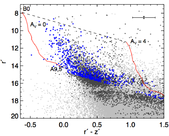
Figure 2: W5 optical photometric sample (light gray points) overlaid with dark gray points showing spectral sample.  Blue points mark A and B stars in the spectral catalog that fall within the extinction limit. A typical error bar is shown in upper right.

3.2 The Age of W5

The full spectroscopic sample in W5 comprises 4800 stars, ranging in spectral type from O9 to M6.5. Since we don’t have a good technique to establish membership of the region, we select objects which match the Spitzer excess source list from Koenig et al. (2008): a total of 389 stars. We calculate for each star the value of optical extinction $A_{V}$ from the observed optical photometry:

$$A_{V}=2.56\left(r^{\prime}-z^{\prime}-\left[1.584(R_{C}-I_{C})-0.386\right]\right)$$ (1)

We obtain $R_{C}-I_{C}$ from Kenyon & Hartmann (1995) according to spectral type. Equation 1 relies on the conversion between $R_{C}I_{C}$ and SDSS $r^{\prime}z^{\prime}$ given in Jordi et al. (2006) and the extinction versus wavelength values given in Schlegel et al. (1998) such that $A_{r^{\prime}}$ = 0.843 $A_{V}$ and $A_{z^{\prime}}$ = 0.453 $A_{V}$.

In Figure 3 (left panel) we present the dereddened optical color-magnitude diagram for this sub-sample. We overplot isochrones at 1, 5 and 100 Myr from Siess et al. (2000), assuming a distance of 2 kpc to W5 and using the conversion relations between $R_{C}I_{C}$ and SDSS $r^{\prime}z^{\prime}$ from Jordi et al. (2006). The distribution of the later spectral type stars at $(r^{\prime}-z^{\prime})_{0}>0.3$ suggests that W5 is at age 5 Myr or younger. This compares well with the age upper limit implied by the presence of the central O stars in the region (5 Myr, Karr & Martin, 2003) and with the bubble expansion ages presented in Vallée et al. (1979) (age $<$ 1.4 Myr). However, a trend of increasing stellar age with increasing mass is apparent in Fig. 3. In the right panel of the figure we show a zoomed-in portion of the diagram focusing on the massive stars, with A and B stars highlighted in blue. In this part of the color-magnitude diagram the stars lie fainter than where we would expect them at an age of 5 Myr given the models of Siess et al. (2000). Some small fraction of these objects may be background stars, but some are likely intrinsically fainter than the model prediction. This result is a common property of stellar ages derived using the HR diagram as noted by Hillenbrand et al. (2008). We believe this does not indicate a true difference in the ages of the low and high mass stars in W5.

The spectral sample was of sufficient resolution to detect Lithium $\lambda$6707 absorption, an indicator of youth (Randich et al., 2001; Hartmann, 2003) in 15 of these objects. We highlight these stars with green boxes in Figure 3.

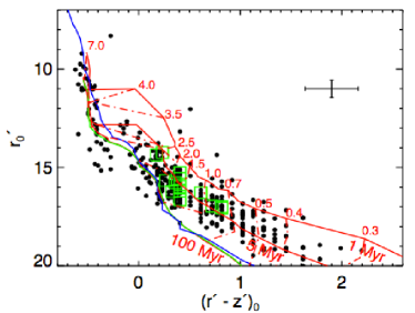
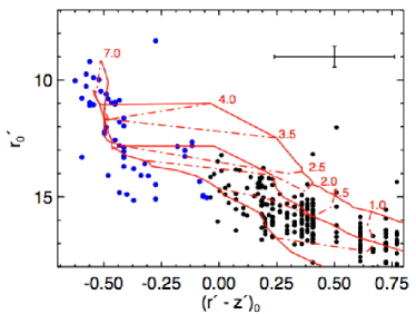
Figure 3: Left panel: dereddened color-magnitude diagram for all Spitzer excess sources (Koenig et al. 2008) detected in our spectroscopic survey. Green boxes indicate those objects with convincing Lithium absorption. Solid red lines: isochrones at 1, 5 and 100 Myr from Siess et al. (2000). Solid blue line: Main Sequence from Kenyon & Hartmann (1995) and Schmidt-Kaler (1982); solid green line: Main Sequence from Siess et al. (2000). Right panel: zoomed-in portion showing the A and B stars highlighted with blue points. A typical error bar is shown in upper right of each panel.

We present the photometry and derived spectral types, H$\alpha$ equivalent widths (EW) and $A_{V}$ extinction values for the list of 389 IR excess stars with spectral types described above in Table 1. Column 14 gives the spectral type and its respective error for each star. The uncertainty is a combination of error from the fit of each index to the standard main sequence and the error in the measurement of each index. We measured the equivalent width of the H$\alpha$ line using the splot task in the IRAF spectral reduction package noao.onedspec. In those cases where both emission and absorption components were visible in the spectrum, the EW was measured across the full line profile. The EW(H$\alpha$) is given in column 15 of Tab. 1. We list the extinction $A_{V}$ in column 16.

Table 1: W5 IR Excess Spectral Catalog

	RA	Dec	$J$	$H$	$K_{S}$	$[3.6]$	$[4.5]$	$[5.8]$	$[8.0]$	$[24]$	$r^{\prime}$	$z^{\prime}$	Sp. Type	EW(H$\alpha$)	$A_{V}$
ID	(deg)	(deg)	(mag)	(mag)	(mag)	(mag)	(mag)	(mag)	(mag)	(mag)	(mag)	(mag)	Type	(Å)	(mag)
1141	41.831320	60.498171	14.11(04)	13.38(03)	13.01(03)	12.52(01)	12.34(01)	10.35(01)	8.41(01)	5.98(15)	17.06(12)	15.89(12)	A8.0$\pm$1.0	8.12	3.22(50)
1473	41.922683	60.521748	14.05(04)	13.13(04)	12.30(03)	11.13(00)	10.78(00)	10.47(01)	9.91(01)	5.76(05)	17.21(12)	16.06(12)	F6.0$\pm$1.0	0.32	2.77(50)
1562	41.952386	60.964075	12.04(02)	10.94(02)	9.96(02)	8.85(00)	8.55(00)	8.08(00)	7.11(00)	3.59(07)	14.06(12)	13.50(12)	B9.0$\pm$0.5	-46.50	2.48(50)
1576	41.958330	60.679266	14.64(03)	13.93(04)	13.59(04)	13.41(01)	13.07(01)	13.38(07)	$\cdots$	$\cdots$	18.17(12)	16.52(13)	A1.0$\pm$0.5	4.31	5.19(52)
1675	41.986977	60.502611	16.26(11)	14.93(09)	14.22(06)	13.22(02)	12.87(01)	12.46(04)	11.85(08)	8.87(16)	18.58(15)	17.84(13)	M7.0$\pm$1.0	-26.38	$\cdots$
1848	42.036912	60.338789	14.45(03)	13.40(03)	13.08(03)	12.79(01)	12.75(01)	12.43(05)	11.76(12)	$\cdots$	18.50(12)	16.61(12)	K3.5$\pm$1.0	2.27	3.82(51)
1970	42.078841	60.337579	13.56(02)	13.12(02)	12.93(02)	12.78(01)	12.72(01)	12.40(09)	11.52(14)	$\cdots$	15.90(12)	15.12(12)	B9.0$\pm$0.5	9.35	3.06(50)
2068	42.115392	60.711151	13.92(03)	12.83(03)	12.05(02)	10.70(00)	10.02(00)	9.11(00)	7.58(01)	4.46(03)	17.33(12)	15.96(12)	F7.5$\pm$1.0	-27.17	3.22(50)
2234	42.175010	60.686677	14.04(03)	13.63(04)	13.49(04)	13.48(01)	13.45(01)	13.11(07)	12.77(20)	$\cdots$	15.71(12)	15.27(12)	F3.5$\pm$0.5	3.77	1.15(50)
2309	42.204412	60.792946	13.52(03)	12.55(03)	11.76(02)	10.31(00)	9.93(00)	9.60(01)	8.96(01)	4.92(06)	17.22(12)	15.61(12)	G7.0$\pm$1.0	-2.50	3.58(50)

Note. — This Table is published in its entirety in the electronic edition of the Astrophysical Journal. A portion is shown here for guidance regarding its form and content. Values in parentheses by photometry signify error in last two digits of magnitude value. Right Ascension and Declination coordinates are J2000.0. Please contact author for full table.

3.3 Disk Classification

We aim to quantify the relative fractions of different disk morphologies among the A and B stars in W5. The infrared spectral energy distributions of young stars can show a wide variety of morphologies, depending on the properties and evolutionary stage of the disk. In order to display this information, for each star we calculate the excess as a function of wavelength by deriving: $(J-[\lambda])_{dered}-(J-[\lambda])_{phot}$, i.e. the dereddened color at wavelength $\lambda$ minus the photospheric contribution at that wavelength. We assume that there is little or no excess emission at $J$ band. The photospheric colors for a given spectral type are calculated by convolving a simple Planck function at the stellar effective temperature given in Schmidt-Kaler (1982) with the appropriate filter-plus-telescope-plus-instrument response curves (as archived for 2MASS and Spitzer  ). The colors derived by our blackbody calculation agree with those in the literature, for example: Bessell & Brett (1988), within 0.05 mag. We use the infrared extinction law $A_{[\lambda]}/A_{V}$ given by Indebetouw et al. (2005) at near-infrared wavelengths and Flaherty et al. (2007) in the Spitzer bands to deredden our infrared photometry for this calculation. We require that objects possess a 3$\sigma$ excess in at least one filter to qualify as an excess object. Upper limit detections were not acceptable as evidence of an excess and we also reject objects that are visibly non-point-like in either the 8 or 24 $\micron$ images.

We identify four morphological classes based on the wavelength dependence of the observed excess emission above theoretical photospheric levels: (a) optically thick disks that resemble the known class of Herbig AeBe stars; (b) disks with an optically thin excess over the wavelength range 2 to 24 $\micron$, similar to that shown by Classical Be stars; (c) disks that are optically thin in their inner regions based on their infrared excess at 2–8 $\micron$ and optically thick in their outer regions based on the magnitude of the observed excess emission at 24 $\micron$; (d) disks that exhibit empty inner regions (no excess emission at $\lambda\leq$8 $\micron$) and some measurable excess emission at 24 $\micron$. A sub-class of disks exhibit no significant excess emission at $\lambda\leq$5.8 $\micron$, have excess emission only in the Spitzer 8 $\micron$ band and no detection at 24 $\micron$.

There already exists a plethora of classifications for disks around young stars, in particular for low mass stars (M${}_{\star}\leq$1 M_⊙) and the classes we have found in the A and B stars in W5 should be put into this context. In the low mass case, SEDs are classified according to their slope in the near to mid infrared into Class I (an optically thick disk and an envelope), Class II (an optically thick disk), Class III (no infrared excess) and ‘transitional disks’ (no infrared excess shortward of 24 $\micron$). Lada et al. (2006) found a further SED morphology of optically thin excesses in the IC 348 cluster that they labeled ‘anemic’ disks. A and B star disks in type (a) resemble the low mass Class I and II disks. Our type (b) disks are similar to the anemic disks seen in IC 348. The type (d) disks resemble the ‘transitional’ disks in low mass stars. The thin/thick disks in type (c) are not exactly like any of these definitions of disks, but a similar type was noted by Malfait, Bogaert, & Waelkens (1998) in their survey of nearby Herbig AeBe stars.

In Figure 4 we show the excess emission (in magnitudes) over the photospheric level as a function of wavelength for four A and B stars in our spectral sample showing excesses typical of our new classes. In the list of 610 AB stars in the extinction limited sample we found 46 (7.5%) with infrared emission consistent with one of these four morphologies: Optically thick/Herbig AeBe (a), Optically thin (b), Optically thin inner and thick outer (c) and ‘Inner Hole’ (d). The 9 optically thick disks constitute a fraction of 1.5% of the extinction limited sample. The remaining stars not grouped under the four categories above appeared photospheric over the viewable wavelength range although many objects lacked a detection at 8 or 24 $\micron$, thus we are likely missing some disks. Inner hole disks are detected around stars over the spectral type range A8.5 to B0 and mass range 1.6 $<M_{\star}\leq$ 15 $M_{\odot}$.

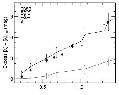
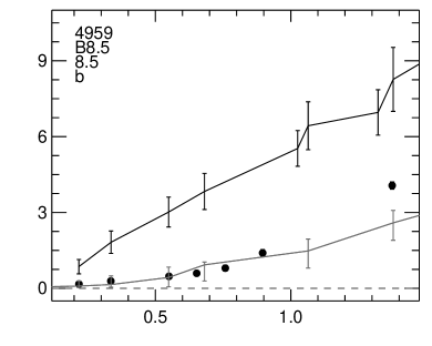
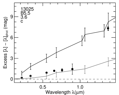
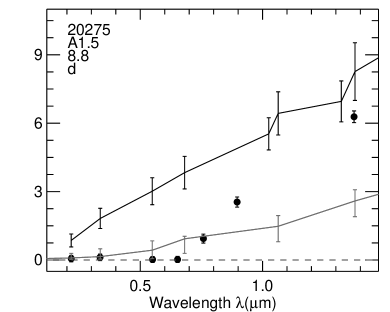
Figure 4: Distribution of excess emission in magnitudes: $[\lambda]_{dered}-[\lambda]_{phot}$ as a function of wavelength for four example stars (remaining objects are shown in the Appendix). Error bars include uncertainty in $A_{V}$ calculation. The zero level represents the photospheric level for that spectral type. In upper left are shown the spectral type and $W({\rm H\alpha})$ in Å. Black line: Herbig AeBe star median and quartiles from Hillenbrand et al. (1992), gray line: CBe star median and quartiles from Coté & Waters (1987), Waters et al. (1987) and Dougherty et al. (1991, 1994).

We present the properties of the 46 spectrally confirmed A and B stars with IR excess in Table 2. IR excess plots for all of these sources are shown in the Appendix, with the letter corresponding to the excess class in upper left of each plot. Disks in the sub-class with excess only at 8 $\micron$ and no 24 $\micron$ detection are marked as ’de’ in the plots.

Table 2: AB Stars With IR Excess

	RA	Dec	$J$	$H$	$K_{S}$	$[3.6]$	$[4.5]$	$[5.8]$	$[8.0]$	$[24]$	$r^{\prime}$	$z^{\prime}$	Sp. Type	EW(H$\alpha$)	$A_{V}$
ID	(deg)	(deg)	(mag)	(mag)	(mag)	(mag)	(mag)	(mag)	(mag)	(mag)	(mag)	(mag)	Type	(Å)	(mag)	Disk
9046	43.495831	60.666310	11.00(02)	10.43(03)	9.68(02)	8.49(00)	8.00(00)	7.49(00)	6.93(00)	5.48(07)	12.62(12)	12.24(12)	B8.5$\pm$0.5	6.42	2.08(50)	a
16953	45.339983	60.482399	11.79(03)	10.80(03)	9.87(02)	8.57(00)	8.08(00)	7.44(00)	6.30(00)	3.69(07)	14.04(12)	13.44(12)	B8.5$\pm$0.5	-17.82	2.67(50)	a
1562	41.952386	60.964075	12.04(02)	10.94(02)	9.96(02)	8.85(00)	8.55(00)	8.08(00)	7.11(00)	3.59(07)	14.06(12)	13.50(12)	B9.0$\pm$0.5	-46.50	2.48(50)	a
5084	42.808983	60.374804	11.68(03)	11.12(03)	10.44(02)	9.12(00)	8.60(00)	8.19(00)	7.70(00)	6.27(05)	13.23(12)	12.90(12)	B9.0$\pm$0.5	-0.42	1.91(50)	a
6388	43.009641	60.604807	14.03(04)	13.35(05)	$\cdots$	10.60(00)	10.16(00)	9.73(01)	8.51(01)	4.96(05)	16.25(12)	15.49(12)	B9.0$\pm$0.5	-8.40	3.03(50)	a
15405	44.933304	60.541502	13.23(02)	12.48(03)	11.60(02)	10.29(00)	9.70(00)	8.97(00)	7.63(00)	4.90(04)	15.11(12)	14.73(12)	A2.5$\pm$0.5	-14.19	1.80(50)	a
5232	42.827700	60.346598	12.50(03)	12.05(04)	11.60(02)	10.65(00)	10.16(00)	9.77(01)	9.09(00)	7.71(06)	14.15(12)	13.73(12)	A6.0$\pm$0.5	5.83	1.55(50)	a
2736	42.341200	60.751156	13.16(03)	12.11(04)	11.08(02)	9.95(00)	9.55(00)	9.05(01)	8.11(02)	4.23(08)	15.97(12)	14.75(12)	A6.5$\pm$0.5	-11.87	3.51(50)	a
7717	43.254185	60.595434	12.66(02)	11.99(03)	11.34(02)	10.24(00)	9.81(00)	9.20(00)	7.74(00)	4.71(08)	14.55(12)	14.11(12)	A6.5$\pm$0.5	-2.40	1.52(50)	a
13385	44.461729	60.330359	10.71(04)	10.46(05)	10.37(04)	9.89(00)	9.71(00)	9.49(01)	9.25(02)	7.25(18)	11.90(12)	11.66(12)	B0.0$\pm$0.5	-12.20	2.23(50)	b

Note. — This Table is published in its entirety in the electronic edition of the Astrophysical Journal. A portion is shown here for guidance regarding its form and content. Values in parentheses by photometry signify error in last two digits of magnitude value. Right Ascension and Declination coordinates are J2000.0. Please contact author for full table.

The breakdown of infrared excess types in our spectral sample is presented in Table 3. Following the findings of Wolff et al. (2010, in press) we also note a further sub-category of group (d) that is: objects with no discernible excess in wavebands up to 5.8 $\micron$ and a real 3$\sigma$ excess at the 8 $\micron$ band. We find three such objects in the W5 sample and mark them as ‘de’ in Table 2. These may be examples of a disk with a central hole, or objects with strong PAH line emission (which would give rise to a sharp increase at 8 $\micron$ but not at shorter wavelengths).

We next expand our sample of intermediate mass stars in W5 by adding candidate A and B stars from the full $J$ through 24 $\micron$ photometric catalog of Koenig et al. (2008) that were not included in the spectroscopic survey. We choose objects with $J$-band and IRAC channel 1 to 4 photometric uncertainty $\leq$0.2, a total of 14283 stars, excluding the list for which we have already obtained spectra. As described by Koenig et al. we estimate the extinction for each source in the absence of a spectral type from an $A_{V}$ map constructed with 2MASS $HK_{S}$ photometry of sources across W5. We deredden the photometry with the value of $A_{V}$ given by the location of each source within the map. We assume that A and B stars at the distance of W5 will have a dereddened $J$ magnitude $\leq$13 and use this limit as a first cut to find them in the photometric sample: a total of 4805 candidate A and B stars. In Figure 5 we show a dereddened plot of 2MASS $J-H$ versus $J$ for the spectroscopic sample of A and B stars (with extinction as calculated in $\S$ 2.4) and for the photometric sample in W5 dereddened with the extinction map as described in Koenig et al. (2008).

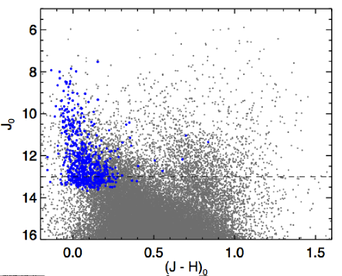
Figure 5: Dereddened 2MASS $J$ and $H$ color-magnitude diagram for spectroscopically confirmed A and B stars (blue points) and the photometric sample in W5 (dark gray points). Photometry is dereddened for spectroscopically confirmed A and B stars as in $\S$ 2.4, and for the photometric points with the extinction map of Koenig et al. (2008). Dashed line shows the cut we make in the photometric data to isolate candidate A and B stars at the distance of W5.

The $J_{0}$=13 limit roughly corresponds to a main-sequence star of spectral type A5 at 2 kpc (Schmidt-Kaler, 1982; Kenyon & Hartmann, 1995). With the spectral sample as a guide, we examine the infrared colors of sources brighter than this and classify them into the same IR SED groups by their location in color space in Figure 6. We only include objects with an excess in at least one color: a total of 64 objects, as before excluding stars for which we already have spectra. The full classification scheme is described in the Appendix. Table 3 presents the resulting breakdown of disks in the photometric sample by type. The candidate photometric A and B stars with IR excess are plotted in Fig. 6 (lower panels).

The method of finding the photometric-only sample of A and B stars is crude since we only require they be bright and possess an apparent infrared excess. As a test, we applied the same criteria to our spectroscopic catalog of 4800 objects and found 60 objects. Of these stars 62% proved to be A or B type, since some later type stars can be similarly bright and possess excess infrared emission. The contamination fraction is not constant between the different disk types. The fraction of confirmed A and B stars by group was: Thick: 50%, Thin: 63%, Thin/Thick: 45%, Hole: 83%. We add a further row to Table 3 applying these success rates to the photometric sample. We note that the proportions of the different disk types are consistent within the errors.

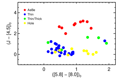
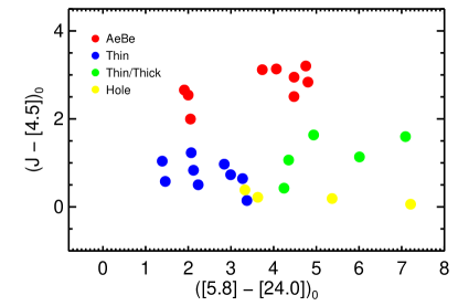
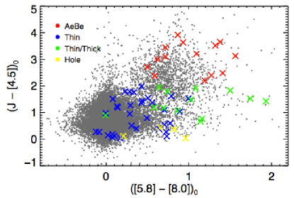
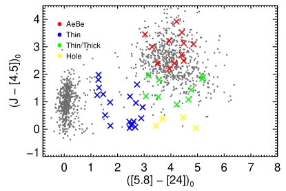
Figure 6: Upper panels: Color-color diagrams for the spectroscopic sample of A and B stars in W5 possessing at least a 3 sigma excess in one or more bands, color-coded according to disk class. Red: type (a), blue: type (b), green: type (c), yellow: type (d). Lower panels: Color-color diagrams for the photometric sample in W5: gray points show all photometric detections, colored crosses show best candidate A and B stars with the same color scheme as for the spectroscopic sample.

Table 3: Disk Type Breakdown

	HAeBe	Thin	Thin/Thick	Hole
Spectral	9	23	5	9
Photometric	14	33	13	4
Total	23	56	18	13
(%)	21$\pm$4.8	51$\pm$8.4	16$\pm$4.2	12$\pm$3.5
Alt. Total	16	44	11	12
(%)	19$\pm$5.3	53$\pm$9.9	13$\pm$4.3	15$\pm$4.5

3.4 Accretion Signatures in the AB star sample

The spectra in this paper have insufficient resolution to precisely measure H$\alpha$ equivalent widths (EW(H$\alpha$) and are subject to large errors introduced by our crude sky subtraction technique. Thus we are unable to establish reliable measures of the accretion rates in our sample of A and B star disks. However, we can still use the measurements of EW(H$\alpha$) from our spectra to assess to first order which of the stars exhibit some noticeable excess emission and are still accreting.

In Figure 7 we plot the measured EW(H$\alpha$) as a function of effective temperature for all of the A and B stars in the spectral sample. We overlay on this plot the disk excess objects, color-coded according to our earlier color scheme. Negative values of EW(H$\alpha$) indicate emission lines.

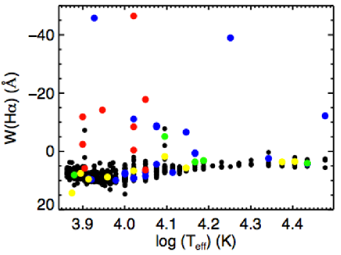
Figure 7: H$\alpha$ equivalent width as a function of effective temperature for the A and B stars in our sample. Objects showing disk excess are color-coded according to the color scheme established in Figure 6.

The Main Sequence level of H$\alpha$ absorption is clearly traced from $\sim$10 Å in the A stars below 10000 K to $\sim$5 Å in the hottest B stars at 30000 K. The largest negative values of EW(H$\alpha$) (corresponding to emission) are in the thick disk and thin disk sources. In the case of the thick disk sources this emission is likely produced by accretion from the circumstellar disk. One of the ‘thick’ objects (ID 5267, a B5.5 star) was observed at multiple epochs (7-Oct-2007 and 30-Sept-2008). Its H$\alpha$ equivalent width varied from -7.99 to 0.49 Å between these two observations, suggesting variable accretion activity in this source. The ‘thin’ sources’ SEDs resemble those of Classical Be stars which exhibit strong emission in this line produced in a stellar wind (Porter & Rivinius, 2003). The thin/thick and hole sources also exhibit some evidence for H$\alpha$ in emission which suggests that some of these stars may still be accreting material from their disks but clearly at a consistently lower rate than in the thick disks.

3.5 Spatial Variation in SED types

We present the spatial distribution of A and B star disks in W5 in Figure 8 on the Spitzer MIPS 24 $\micron$ mosaic. We find no systematic trends of location with disk type, however we note that the high extinction on the molecular clouds (marked by the bright diffuse 24 $\micron$ emission around the rim of W5) will strongly reduce the number of disk excess objects we find in our survey in these regions. In Koenig et al. (2008) we calculated the 90% completeness limits for our Spitzer survey as a function of location and wavelength. In the H ii region cavities we find 90% limits of 16.1 (4.5 $\micron$), 14.6 (5.8 $\micron$), 13.4 (8 $\micron$) and 11.2 (MIPS, 24 $\micron$). In the bright diffuse emission regions, the limits are: 14.2 (4.5 $\micron$), 12.3 (5.8 $\micron$), 9.5 (8 $\micron$) and 8.5 (MIPS, 24 $\micron$). Adopting theoretical colors as calculated in $\S$3.3 these results mean we are able to detect all A and B star excess types in the H ii region cavities. On the cloud however, we are limited by a convolution of the detection limits in each band with the range of excesses for each disk type. Table 4 presents a summary of the resulting completeness limits. As a consequence we miss almost all A-type Thin and Hole disk sources against the bright cloud diffuse emission.

Table 4: Disk Type Completeness

	Thick Disks	Thin Disks	Thin/Thick Disks	Hole Disks
90% Completeness Limit	A9.5	A0	A9.5	A0
Brightest 50% Only	N/A	A1	N/A	A4.5

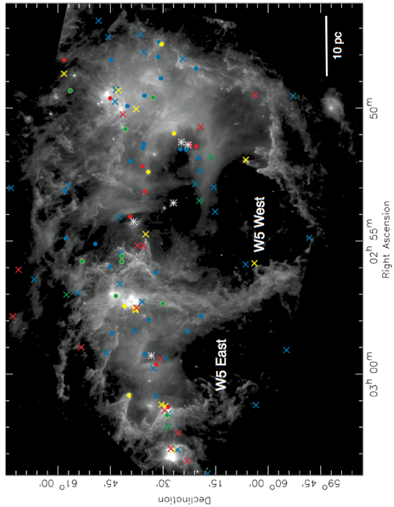
Figure 8: Spitzer MIPS 24 $\micron$ mosaic overlaid with AB star disk candidates. Dot points show spectroscopically confirmed A and B stars. Cross points mark photometric-only sources. Color-coding is as in Fig. 6. Known O stars in W5 are marked with white asterisks.

4 Discussion

We have found a sample of young A and B stars in W5 that possess a variety of disk morphologies and that the disks can be grouped into four distinct types. Although this scheme is a crude way to describe what is almost certainly a continuum of disk morphologies, we can use these types to investigate the properties and origins of these disks. Indeed a similar scheme was constructed by Malfait, Bogaert, & Waelkens (1998) from their observations of near and mid-infrared excesses in nearby A and B stars. We have been able to note this same range of disk types in a single young region.

We firstly assume that all stars of intermediate mass begin their life in a protostellar phase similar to that of low mass stars. As such, they initially possess an accretion disk and an infalling envelope. As time progresses, the envelope disappears and an optically thick accretion disk is left behind. Andrews & Williams (2007) and Muzerolle et al. (2000) have shown that in low mass stars, the disk-to-star mass ratio can span two orders of magnitude (from 0.1 to 10% of the stellar mass) as can the disk accretion rate onto the star. If the same property applies to intermediate mass stars, then the initial conditions alone can produce very different end states after a given amount of time in the AB stars’ disks in a cluster as these disks drain onto their stars and dissipate through spreading.

Viscous draining and spreading of a disk alone are likely too slow to explain observed disk evolutionary timescales (Hartmann et al., 1998). Several additional mechanisms exist that will alter the evolution of the star-disk system in time and operate on more rapid timescales. The disk may photoevaporate due to radiation from the host or external stars. Dust grains in the disk can settle to the mid-plane and grow in size. Finally, large solid bodies (planetesimals and planets) may form in the disk. There is evidence that disk evolution proceeds faster in more massive stars than in low mass stars (Haisch et al., 2001). Hernández et al. (2005) suggest that the timescale for removal of the optically thick inner disk in Herbig Ae/Be stars (types B5 to A9) is short, given that the fraction of stars with an optically thick inner disk as seen in the $JHK_{S}$ bands is lower at a given age amongst A and B stars than in low mass GKM stars. In W5 we find no optically thick disks in our spectral sample in stars earlier than B8.5. Put another way, only 20$\pm$5% of stars with any kind of excess are still optically thick in the spectroscopic-only sample, and none above a mass 2.4 $M_{\odot}$.

External erosion of low mass star disks has been clearly observed in the Orion Nebula near the Trapezium stars (O’Dell et al., 1993), but the expected photoevaporation rate produced drops off exponentially with distance if the star and disk are beyond 1 pc from the powering O star. Photoevaporation of the disk by its host star is driven by heating of the disk surface by X-ray (h$\nu>$0.1 keV), Far-ultraviolet (FUV, h$\nu<$13.6 eV) and Extreme ultraviolet (EUV, h$\nu>$13.6 eV) radiation. FUV radiation heats the disk. Beyond a certain radius in the disk, the gas thermal velocity exceeds the escape velocity of the system and material can leave in a photoevaporative wind. This effect removes the outer disk while the inner disk drains onto the star through accretion. X-rays and EUV radiation may be able to create a gap in the disk and subsequently rapidly clear the entire inner disk (Clarke et al., 2001). Key to the operation of this mechanism is the ability of the EUV and X-ray photons to penetrate the accretion flow and ionize the disk—a still open question (Ercolano et al., 2008). A disk cleared out from the inside in this manner might resemble the ‘inner hole’ sources in our survey. The timescale for this process is short however, typically less than 10⁵ yr (Alexander et al., 2006).

As a disk evolves, dust grains will settle to the disk mid-plane and can grow in size. Grain growth and planetesimal formation will reduce the optical depth in small grains which could explain the reduced emission in the inner disk as seen in the thin/thick sources. Gas will still be present in such a disk and so the accretion rate should remain at a similar level as in the optically thick disks. The formation of a giant planet in the disk (M$\approx$M_Jup) could also produce the thin/thick morphology. The planet both reduces the dust optical depth and decreases the accretion rate of material onto the star by slowing the rate of flow of material from the outer to the inner disk (Rice et al., 2006). In this case the accretion rate will be around 10% of the typical thick disk rate. A large enough planet (M$\gg$M_Jup) can completely clear the inner disk, resulting in a disk more like the ‘hole’ sources. A study of the disks around low mass stars in Taurus appears to show that stars with IR morphologies similar to our thin/thick sources do indeed have accretion rates about 10$\times$ lower than the optically thick accretion disks (Najita, Strom & Muzerolle, 2007). If the same is true for the AB stars in W5, then these sources may be good candidates for giant-planet forming disks. The H$\alpha$ line in the thin/thick sources are systematically smaller than in the thick sources in Fig. 7, however these results are not precise enough to establish their relative accretion rates. The hole sources are similar to the thin/thick disks in that they show some process that has cleared out the inner disk. These could be examples of giant planet formation as well, but could also simply be photoevaporated disks. Again their H$\alpha$ lines show less emission than the thick disk sources which could indicate lower accretion rates in these objects.

The thin disk objects in our sample resemble so-called homologously depleted or weak disks. These disks may represent the action of grain growth or some process that drives mass loss from the disk at a wide range of disk radii. Luhman et al. (2010) and Muzerolle et al. (2010) discovered similar disks in their recent studies of low mass young stars, but in far fewer numbers. In Figure 9 we make a plot similar to their Figures 18–25. They typically find $<$10 objects below the boundary marking the location of Taurus primordial disks (with the exception of the sample from IC 348). As a fraction of all disks, our sample of thin disks in W5 is larger than in any of their low mass disk samples. We do not know at present why they are more prevalent among young intermediate mass stars. The earliest types showing this excess are a B0, a B0.5 and a B2 star.

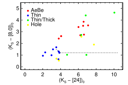
Figure 9: $K_{S}-[8.0]vs.K_{S}-[24]$ color-color plot of spectroscopic A and B stars in W5, analogous to Figures 18 to 25 in Luhman et al. (2010). The lower boundary of primordial disks in Taurus that they identify is shown as a dotted line.

5 Conclusions and Future Work

We have carried out a combined infrared and optical photometric and spectroscopic survey of young stars in W5. We present evidence from the larger spectroscopic sample that W5 is a young region (age $\lesssim 5$ Myr), in agreement with the presence of massive O stars and a short expansion timescale for the H ii region bubbles. More detailed analysis of the HR diagram would help to place better constraints on the age of W5.

Within the spectroscopic sample we identify a population of A and B stars. Of these, we find that 46 objects show excess infrared emission in at least one Spitzer band. We find that many of these infrared excess sources suggest evolved disks with little or no excess infrared emission above the photosphere up to a wavelength 5.8–8 $\micron$, but strong excess at longer wavelengths. These may be transitional disk objects that have cleared out their inner disks. Photoevaporation is one possible mechanism to create this SED morphology, however there is a distinct possibility that their SEDs are produced by the formation of one or more planets. If we can assess the contribution of the various mechanisms of disk evolution and their frequency of occurence, we can begin to understand what types of planets will form in a given disk around a star of given mass, how frequently planet formation occurs in the Galaxy and at what point in a star’s evolution it begins. A clearer picture of the planet forming potential of intermediate mass stars should soon emerge.

Appendix A Disk Classification Scheme

We classify disks from the photometric sample of stars possessing dereddened $J$ magnitudes brighter than 13 according to the following scheme using dereddened photometry in all cases. Firstly we identify Herbig AeBe star candidates.

$$J-[4.5]>2.0$$ (A1)

$$[5.8]-[8.0]>0.3$$ (A2)

$$J-H>\frac{0.7}{0.55}(H-K_{S})-0.6$$ (A3)

$$J-H>-\frac{0.25}{0.28}(H-K_{S})-0.59$$ (A4)

$$J-H>\frac{0.95}{0.55}(H-K_{S})-0.116$$ (A5)

$$J-H<1.2$$ (A6)

Next we identify the ‘thin’ disk candidates:

$$J-[4.5]>-4.5([5.8]-[8.0])+3.0$$ (A7)

$$-0.25<J-[4.5]\leq 2.0$$ (A8)

and either:

$$[5.8]-[8.0]\leq 1.0$$ (A9)

or:

$$1.2<[5.8]-[24.0]\leq 3.0$$ (A10)

We next pick out the ‘thin/thick’ sources. In some cases this re-classifies thin-disk sources.

$$0.5<J-[4.5]\leq 2.0$$ (A11)

and either:

$$[5.8]-[8.0]>1.0$$ (A12)

or:

$$[5.8]-[24.0]>3.0$$ (A13)

Lastly we find the ‘hole’ sources:

$$-0.25\leq J-[4.5]\leq 0.5$$ (A14)

and either:

$$[5.8]-[8.0]>1.0$$ (A15)

or:

$$[5.8]-[24.0]>3.0$$ (A16)

Appendix B IR Excess Plots

In Figure 10 we display IR excess plots for all of the remaining 42 spectrally confirmed A and B stars that belong to groups a, b, c or d. Sources are listed by group, and within each of these divisions are sorted by spectral type. Every plot also is overlaid with the Group I Herbig AeBe star median and quartiles from Hillenbrand et al. (1992), and a line showing the Classical Be star median and quartiles from Coté & Waters (1987), Waters et al. (1987) and Dougherty et al. (1991, 1994), where the excesses used to find the medians are calculated in the same way as for the W5 stars.

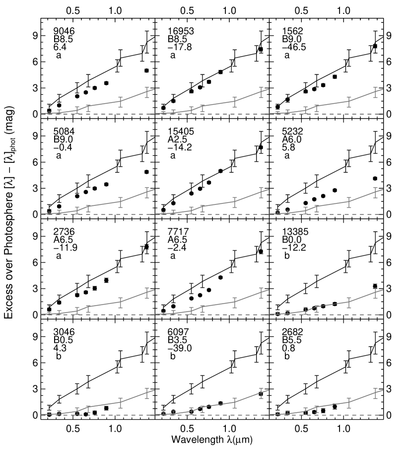
Figure 10: IR Excess plots for the spectrally confirmed A and B stars with infrared excess. Black points show the data and 1$\sigma$ error bars. Upper line and error bars shows Group 1 Herbig AeBe star median and quartiles from Hillenbrand et al. (1992), lower line and error bars shows the Classical Be star median and quartiles from Coté & Waters (1987), Waters et al. (1987) and Dougherty et al. (1991, 1994). In upper left of each plot is given the source ID, spectral type, EW(H$\alpha$) and disk type.

References

- Allen et al. (2005) Allen, L. E., et al. 2005, in IAU Symposium, Vol. 227, Massive Star Birth: A Crossroads of Astrophysics, ed. R. Cesaroni, M. Felli, E. Churchwell, & M. Walmsley, 352–357
- Alexander et al. (2006) Alexander, R. D., Clarke, C. J., & Pringle, J. E. 2006, MNRAS, 369, 229
- Andrews & Williams (2007) Andrews, S. M., & Williams, J. P. 2007, ApJ, 659, 705
- Andrillat et al. (1995) Andrillat, Y., Jaschek, C., & Jaschek, M. 1995, A&AS, 112, 475
- Bessell & Brett (1988) Bessell, M. S., & Brett, J. M. 1988, PASP, 100, 1134
- Carquillat et al. (1997) Carquillat, M. J., Jaschek, C., Jaschek, M., & Ginestet, N. 1997, A&AS, 123, 5
- Clarke et al. (2001) Clarke, C., Gendrin, A., & Sotomayor, M. 2001, MNRAS, 328, 485
- Coté & Waters (1987) Coté, J. & Waters, L. B. F. M. 1987, A&A, 176, 93
- Dougherty et al. (1991) Dougherty, S. M., Taylor, A. R., & Clark, T. A. 1991, AJ, 102, 1753
- Dougherty et al. (1994) Dougherty, S. M., Waters, L. B. F. M., Burki, G., Coté, J., Cramer, N., van Kerkwijk, M. H., & Taylor, A. R. 1994, A&A, 290, 609
- Ercolano et al. (2008) Ercolano, B., Drake, J. J., Raymond, J. C., & Clarke, C. C., 2008, ApJ, 688, 398
- Fabricant (1994) Fabricant, D. 1994, FAST Manual (Mount Hopkins: SAO), http://linmax.sao.arizona.edu/help/FLWO/60/fast
- Fabricant et al. (1998) Fabricant, D., Cheimets, P., Caldwell, N., & Geary, J. 1998, PASP, 110, 79
- Fabricant et al. (1994) Fabricant, D., Hertz, E., & Szentgyorgyi, A. 1994, Proc. SPIE, 2198, 251
- Fazio et al. (2004) Fazio, G. G., et al. 2004, ApJS, 154, 10
- Flaherty et al. (2007) Flaherty, K. M., Pipher, J. L., Megeath, S. T., Winston, E. M., Gutermuth, R. A., Muzerolle, J., Allen, L. E., & Fazio, G. G. 2007, ApJ, 663, 1069
- Gordon et al. (2005) Gordon, K. D., et al. 2005, PASP, 117, 503
- Gutermuth et al. (2004) Gutermuth, R. A., Megeath, S. T., Muzerolle, J., Allen, L. E., Pipher, J. L., Myers, P. C., & Fazio, G. G. 2004, ApJS, 154, 374
- Gutermuth et al. (2008) Gutermuth, R. A., et al. 2008, ApJ, 674, 336
- Haisch et al. (2001) Haisch, K. E., Lada, E. A., & Lada, C. J. 2001, ApJ, 553, L153
- Hartmann et al. (1998) Hartmann, L., Calvet, N., Gullbring, E., & D’Alessio, P. 1998, ApJ, 495, 385
- Hartmann (2003) Hartmann, L. 2003, ApJ, 585, 398
- Hernández et al. (2004) Hernández, J., Calvet, N., Briceño, C., Hartmann, L., & Berlind, P. 2004, AJ, 127, 1682
- Hernández et al. (2005) Hernández, J., Calvet, N., Hartmann, L., Briceño, C., Sicilia-Aguilar, A., & Berlind, P. 2005, AJ, 129, 856
- Hillenbrand et al. (1992) Hillenbrand, L. A., Strom, S. E., Vrba, F. J., & Keene, J. 1992, ApJ, 397, 613
- Hillenbrand (2008) Hillenbrand, L. A. 2008, Phys. Scr., T130, 014024
- Hillenbrand et al. (2008) Hillenbrand, L. A., Bauermeister, A., & White, R. J. 2008, in ASP Conf. Ser. 384, 14th Cambridge Workshop on Cool Stars, Stellar Systems, and the Sun, ed. G. van Belle (San Francisco, CA: ASP), 200
- Indebetouw et al. (2005) Indebetouw, R., et al. 2005, ApJ, 619, 931
- Jacoby et al. (1984) Jacoby, G. H., Hunter, D. A., & Christian, C. A. 1984, ApJS, 56, 257
- Johnson et al. (2007) Johnson, J. A. et al. 2007, ApJ, 665, 785
- Jordi et al. (2006) Jordi, K., Grebel, E. K., & Ammon, K. 2006, A&A, 460, 339
- Karr & Martin (2003) Karr, J. L., & Martin, P. G. 2003, ApJ, 595, 900
- Kenyon & Hartmann (1995) Kenyon, S. J., & Hartmann, L. W. 1995, ApJS, 101, 117
- Koenig et al. (2008) Koenig, X. P., Allen, L. E., Gutermuth, R. A., Hora, J. L., Brunt, C. M., & Muzerolle, J. 2008, ApJ, 688, 1142
- Landsman (1993) Landsman, W. B. 1993, in ASP Conf. Ser. 52: Astronomical Data Analysis Software and Systems II, ed. R. J. Hanisch, R. J. V. Brissenden, & J. Barnes, 246–+
- Lada et al. (2006) Lada, C. J. et al. 2006, ApJ, 131, 1574
- Lilly et al. (1991) Lilly, S. J., Cowie, L. L., & Gardner, J. P. 1991, ApJ, 369, 79
- Luhman et al. (2010) Luhman, K. L., Allen, P. R., Espaillat, C., Hartmann, L., & Calvet, N. 2010, ApJS, 186, 111
- Malfait, Bogaert, & Waelkens (1998) Malfait, K., Bogaert, E., & Waelkens, C. 1998, A&A, 331, 211
- McLeod et al. (2000) McLeod, B. A., Conroy, M., Gauron, T. M., Geary, J. C., & Ordway, M. P. 2000, in Further Developments in Scientific Optical Imaging, ed. M. B. Denton (Cambridge: Royal Society of Chemistry), 11
- Muzerolle et al. (2000) Muzerolle, J., Calvet, N., Briceño, C., Hartmann, L., & Hillenbrand, L. 2000, ApJ, 535, L47
- Muzerolle et al. (2010) Muzerolle, J., Allen, L. E., Megeath, S. T., Hernández, J., & Gutermuth, R. A. 2010, ApJ, 708, 1107
- Najita, Strom & Muzerolle (2007) Najita, J. R., Strom, S. E., & Muzerolle, J. 2007, MNRAS, 378, 369
- O’Dell et al. (1993) O’Dell, C. R., Wen, Z., & Hu, X. 1993, ApJ, 410, 696
- Porter & Rivinius (2003) Porter, J. M., & Rivinius, T. 2003, PASP, 115, 1153
- Randich et al. (2001) Randich, S., Pallavicini, R., Meola, G., Stauffer, J. R., & Balachandran, S. C. 2001, A&A, 372, 862
- Rice et al. (2006) Rice, W. K. M., Armitage, P. J., Wood, K., & Lodato, G. 2006, MNRAS, 373, 1619
- Rieke et al. (2004) Rieke, G. H., et al. 2004, ApJS, 154, 25
- Rivera et al. (2005) Rivera, E. J. et al. 2005, ApJ, 634, 625
- Schlegel et al. (1998) Schlegel, D. J., Finkbeiner, D. P., & Davis, M. 1998, ApJ, 500, 525
- Schmidt-Kaler (1982) Schmidt-Kaler, Th. 1982, in Landolt-Börnstein, Numerical Data and Functional Relationships in Science and Technology, ed. K. Schaifers & H. H. Voigt (Berlin: Springer), 31
- Siess et al. (2000) Siess, L., Dufour, E., & Forestini, M. 2000, A&A, 358, 593
- Skrutskie et al. (2006) Skrutskie, M. F., et al. 2006, AJ, 131, 1163
- Stetson (1987) Stetson, P. B. 1987, PASP, 99, 191
- Strom et al. (1989) Strom, K. M., Strom, S. E., Edwards, S., Cabrit, S., & Skrutskie, M. F. 1989, AJ, 97, 1451
- Szentgyorgyi et al. (2005) Szentgyorgyi, A. H., et al. 2005, BAAS, 37, 1339
- Tokarz & Roll (1997) Tokarz, S. P., & Roll, J. 1997, in ASP Conf. Ser. 125, Astronomical Data and Software Systems VI, ed. G. Hunt & H. E. Payne (San Francisco:ASP), 140
- Vallée et al. (1979) Vallée, J. P., Hughes, V. A., & Viner, M. R. 1979, A&A, 80, 186
- Waters et al. (1987) Waters, L. B. F. M., Coté, J., & Lamers, H. J. G. L. M. 1987, A&A, 185, 206
- Westerhout (1958) Westerhout, G. 1958, Bull. Astron. Inst. Netherlands, 14, 215