Electron-lattice and strain effects in manganite heterostructures: the case of a single interface

Abstract

A correlated inhomogeneous mean-field approach is proposed in order to study a tight-binding model of the manganite heterostructures $(LaMnO_{3})_{2n}/(SrMnO_{3})_{n}$ with average hole doping $x=1/3$. Phase diagrams, spectral and optical properties of large heterostructures (up to $48$ sites along the growth direction) with a single interface are discussed analyzing the effects of electron-lattice anti-adiabatic fluctuations and strain. The formation of a metallic ferromagnetic interface is quite robust with varying the strength of electron-lattice coupling and strain, though the size of the interface region is strongly dependent on these interactions. The density of states never vanishes at the chemical potential due to the formation of the interface, but it shows a rapid suppression with increasing the electron-lattice coupling. The in-plane and out-of-plane optical conductivities show sharp differences since the in-plane response has metallic features, while the out-of-plane one is characterized by a transfer of spectral weight to high frequency. The in-plane response mainly comes from the region between the two insulating blocks, so that it provides a clear signature of the formation of the metallic ferromagnetic interface.

I Introduction

Transition metal oxides are of great current interest because of the wide variety of the ordered phases that they exhibit and the strong sensitivity to external perturbations. imada Among them, manganese oxides with formula $R_{1-x}A_{x}MnO_{3}$ ($R$ stands for a rare earth as $La$, $A$ represents a divalent alkali element such as $Sr$ or $Ca$ and $x$ the hole doping), known as manganites, have been studied intensively both for their very rich phase diagram and for the phenomenon of colossal magnetoresistance. dagotto This effect is often exhibited in the doping regime $0.2<x<0.5$, where the ground state of the systems is ferromagnetic. The ferromagnetic phase is usually explained by invoking the double exchange mechanism in which hopping of an outer-shell electron from a $Mn^{3+}$ to a $Mn^{4+}$ site is favored by a parallel alignment of the core spins. zener In addition to the double-exchange term that promotes hopping of the carriers, a strong interaction between electrons and lattice distortions plays a non-negligible role in these compounds giving rise to formation of polaron quasi-particles. millis

Very recently, high quality atomic-scale ”digital” heterostructures consisting of combination of transition metal oxide materials have been realized. Indeed, heterostructures represent the first steps to use correlated oxide systems in realistic devices. Moreover, at the interface, the electronic properties can be drastically changed in comparison with those of the bulk. Recent examples include the formation of a thin metallic layer at the interface between band and Mott insulators as, for example, between $SrTiO_{3}$ ($STO$) and $LaTiO_{3}$ oxides ohtomo or between the band insulators ohtomo1 $LaAlO_{3}$ and $STO$.

Very interesting examples of heterostructure are given by the superlattices $(LaMnO_{3})_{m}/(SrMnO_{3})_{n}$ with $n/(m+n)$ average hole doping. koida Here $LaMnO_{3}$ ($LMO$) (one electron per $Mn$ $e_{g}$ state) and $SrMnO_{3}$ ($SMO$) (no electrons per $Mn$ $e_{g}$ state) are the two end-member compounds of the alloy $La_{1-x}Sr_{x}MnO_{3}$ and are both antiferromagnetic insulating. In these systems, not only the chemical composition but also the thickness of the constituent blocks specified by $m$ and $n$ is important for influencing the properties of superlattices. Focus has been on the case $m=2n$ corresponding to the average optimal hole doping $x=1/3$. eckstein ; adamo1 The superlattices exhibit a metal-insulator transition as function of temperature for $n\leq 2$ and behave as insulators for $n\geq 3$. The superlattices undergo a rich variety of transitions among metal, Mott variable range hopping insulator, interaction-induced Efros-Shklovskii insulator, and polaronic insulator. adamo2

Interfaces play a fundamental role in tuning the metal-insulator transitions since they control the effective doping of the different layers. Even when the system is globally insulating ($n\geq 3$), some nonlinear optical measurements suggest that, for a single interface, ferromagnetism due to double-exchange mechanism can be induced between the two antiferromagnetic blocks. ogawa Moreover, it has been found that the interface density of states exhibits a pronounced peak at the Fermi level whose intensity correlates with the conductivity and magnetization. eckstein1 These measurements point toward the possibility of a two-dimensional half-metallic gas for the double-layer ogawa1 whose properties have been studied by using ab-initio density functional approaches. nanda However, up to now, this interesting two-dimensional gas has not been experimentally assessed in a direct way by using lateral contacts on the region between the $LMO$ and $SMO$ blocks.

In analogy with thin films, strain is another important quantity in order to tune the properties of manganite heterostructures. For example, far from interfaces, inside $LMO$, electron localization and local strain favor antiferromagnetism and $e_{g}$ ($3z^{2}-r^{2}$) orbital occupation. aruta The magnetic phase in $LMO$ is compatible with the $C$ type. dagotto Moreover, by changing the substrate, the ferromagnetism in the superlattice can be stabilized. yamada

From the theoretical point of view, in addition to $ab$ initio calculations, tight-binding models have been used to study manganite superlattices. Effects of magnetic and electron-lattice interactions on the electronic properties have been investigated going beyond adiabatic mean-field approximations. dagotto1 ; millis1 However, the double layer with large blocks of $LMO$ and $SMO$ has not been much studied. Moreover, the effects of strain have been analyzed only within mean-field approaches. nanda1

In this paper we have studied phase diagrams, spectral and optical properties for a very large bilayer $(LMO)_{2n}/(SMO)_{n}$ (up to size of $48$ planes relevant for a comparison with fabricated heterostructures) starting from a tight binding model. We have developed a correlated inhomogeneous mean-field approach taking into account the effects of electron-lattice anti-adiabatic fluctuations. Strain is simulated by modulating hopping and spin-spin interaction terms. We have found that a metallic ferromagnetic interface forms for a large range of the electron-lattice couplings and strain strengths. For this regime of parameters, the interactions are able to change the size of the interface region. We find the magnetic solutions that are stable at low temperature in the entire superlattice. The general structure of our solutions is characterized by three phases running along growth $z$-direction: antiferromagnetic phase with localized/delocalized (depending on the model parameters) charge carriers inside $LMO$ block, ferromagnetic state at the interface with itinerant carriers, localized polaronic $G$-type antiferromagnetic phase inside $SMO$ block. The type of antiferromagnetic order inside $LMO$ depends on the strain induced by the substrate.

We have discussed the spectral and optical properties corresponding to different parameter regimes. Due to the formation of the metallic interface, the density of states is finite at the chemical potential. With increasing the electron-phonon interaction, it gets reduced at the chemical potential, but it never vanishes even in the intermediate to strong electron-phonon coupling regime. Finally, we have studied both the in-plane and out-of-plane optical conductivities pointing out that they are characterized by marked differences: the former shows a metallic behavior, the latter a transfer of spectral weight at high frequency due to the effects of the electrostatic potential well trapping electrons in $LMO$ block. The in-plane response at low frequency is mainly due to the region between the two insulating blocks, so that it can be used as a tool to assess the formation of the metallic ferromagnetic interface.

The paper is organized as follows: in sec. II the model and variational approach are introduced, in III the results regarding the phase diagrams are discussed, in sec. IV the spectral properties and in sec. V the optical conductivities are analyzed, in the final section the conclusions.

II The variational approach

II.1 Model Hamiltonian

For manganite superlattices, the hamiltonian of the bulk $H_{0}$ has to be supplemented by Coulomb terms representing the potential arising from the pattern of the $La$ and $Sr$ ions, millis2 thus

$$H=H_{0}+H_{Coul}.$$ (1)

In order to set up an appropriate model for the double layer, it is important to take into account the effects of the strain. The epitaxial strain produces the tetragonal distortion of the $MnO_{6}$ octahedron, splitting the $e_{g}$ states into $x^{2}-y^{2}$ and $3z^{2}-r^{2}$ states. nanda1 If the strain is tensile, $x^{2}-y^{2}$ is lower in energy, while, if the strain is compressive, $3z^{2}-r^{2}$ is favored. In the case of $n=8$ and three interfaces, aruta the superlattices grown on $STO$ are found to be coherently strained: all of them are forced to the in-plane lattice parameter of substrate and to an average out-of-plane parameter $c\simeq 3.87\r{A}$. aruta As a consequence, one can infer that $LMO$ blocks are subjected to compressive strain $(-2.2\%)$ and $SMO$ blocks to tensile strain $(+2.6\%)$. For the case of $LMO$ block, the resulting higher occupancy of $3z^{2}-r^{2}$ enhances the out-of-plane ferromagnetic interaction owing to the larger electron hopping out-of-plane. For the case of $SMO$ block, the reverse occurs. A suitable model for the bilayer has to describe the dynamics of the $e_{g}$ electrons which in $LMO$ block and $SMO$ block preferentially occupy the more anisotropic $3z^{2}-r^{2}$ orbitals and more isotropic $x^{2}-y^{2}$ orbitals, respectively. For this reason, in this paper we adopt an effective single orbital approximation for the bulk manganite.

The model for the bulk takes into account the double-exchange mechanism, the coupling to the lattice distortions and the super-exchange interaction between neighboring localized $t_{2g}$ electrons on $Mn$ ions. The coupling to longitudinal optical phonons arises from the Jahn-Teller effect that splits the $e_{g}$ double degeneracy. Then, the Hamiltonian $H_{0}$ reads:

$$H_{0}= -\sum_{\vec{R}_{i},\vec{\delta}}t_{|\vec{\delta}|}\left(\frac{S^{\vec{R}_{i},\vec{R}_{i}+\vec{\delta}}_{0}+1/2}{2S+1}\right)c^{\dagger}_{\vec{R}_{i}}c_{\vec{R}_{i}+\vec{\delta}}$$ (2)

$$+\omega_{0}\sum_{\vec{R}_{i}}a^{\dagger}_{\vec{R}_{i}}a_{\vec{R}_{i}}+g\omega_{0}\sum_{\vec{R}_{i}}c^{\dagger}_{\vec{R}_{i}}c_{\vec{R}_{i}}\left(a_{\vec{R}_{i}}+a^{\dagger}_{\vec{R}_{i}}\right)$$

$$+\frac{1}{2}\sum_{\vec{R}_{i},\vec{\delta}}\epsilon_{|\vec{\delta|}}\vec{S}_{\vec{R}_{i}}\cdot\vec{S}_{\vec{R}_{i}+\vec{\delta}}-\mu\sum_{\vec{R}_{i}}c^{\dagger}_{\vec{R}_{i}}c_{\vec{R}_{i}}.$$

Here $t_{|\vec{\delta}|}$ is the transfer integral of electrons occupying $e_{g}$ orbitals between nearest neighbor ($nn$) sites, $S^{\vec{R}_{i},\vec{R}_{i}+\vec{\delta}}_{0}$ is the total spin of the subsystem consisting of two localized spins on $nn$ sites and the conduction electron, $\vec{S}_{\vec{R}_{i}}$ is the spin of the $t_{2g}$ core states $\left(S=3/2\right)$, $c^{\dagger}_{\vec{R}_{i}}\left(c_{\vec{R}_{i}}\right)$ creates (destroys) an electron with spin parallel to the ionic spin at the i-th site in the $e_{g}$ orbital. The coordination vector $\vec{\delta}$ connects $nn$ sites. The first term of the Hamiltonian describes the double-exchange mechanism in the limit where the intra-atomic exchange integral $J$ is far larger than the transfer integral $t_{|\vec{\delta}|}$. Furthermore, in eq.(2), $\omega_{0}$ denotes the frequency of the local optical phonon mode, $a^{\dagger}_{\vec{R}_{i}}\left(a_{\vec{R}_{i}}\right)$ is the creation (annihilation) phonon operator at the site $i$, the dimensionless parameter $g$ indicates the strength of the electron-phonon interaction. Finally, in Eq.(2), $\epsilon_{|\vec{\delta|}}$ represents the antiferromagnetic super-exchange coupling between two $nn$ $t_{2g}$ spins and $\mu$ is the chemical potential. The hopping of electrons is supposed to take place between the equivalent $nn$ sites of a simple cubic lattice (with finite size along the $z$ axis corresponding to the growth direction of the heterostructure) separated by the distance $|n-n^{\prime}|=a$. The units are such that the Planck constant $\hbar=1$, the Boltzmann constant $k_{B}$=1 and the lattice parameter $a$=1.

Regarding the terms due to the interfaces, one considers that $La^{3+}$ and $Sr^{2+}$ ions act as $+1$ charges of magnitude $e$ and neutral points, respectively. In the heterostructure, the distribution of those cations induces an interaction term for $e_{g}$ electrons of $Mn$ giving rise to the Hamiltonian

$$H_{Coul}= \sum_{\vec{R_{i}}\neq\vec{R_{j}}}\frac{1}{2\epsilon_{d}}\frac{e^{2}n_{\vec{R}_{i}}n_{\vec{R}_{j}}}{|\vec{R_{i}}-\vec{R_{j}}|}+\sum_{\vec{R}_{i}^{La}\neq\vec{R}_{j}^{La}}\frac{1}{2\epsilon_{d}}\frac{e^{2}}{|\vec{R}_{i}^{La}-\vec{R}_{j}^{La}|}$$ (3)

$$-\sum_{\vec{R}_{i},\vec{R}_{j}^{La}}\frac{1}{\epsilon_{d}}\frac{e^{2}n_{\vec{R}_{i}}}{|\vec{R}_{i}-\vec{R}_{j}^{La}|},$$

with $n_{\vec{R}_{i}}=c^{{\dagger}}_{\vec{R}_{i}}c_{\vec{R}_{i}}$ electron occupation number at $Mn$ site $i$, $\vec{R}_{i}$ and $\vec{R}_{i}^{La}$ are the positions of $Mn$ and $La^{3+}$ in $i$th unit cell, respectively, and $\epsilon_{d}$ is the dielectric constant of the material. In our calculation the long-range Coulomb potential has been modulated by a factor $\eta$ inducing a fictitious finite screening-length (see Appendix A). This factor was added only for computational reasons since it allows to calculate the summations of the Coulomb terms over the lattice indices. We have modeled the heterostructures as slabs whose in-plane size is infinite.

In order to describe the magnitude of the Coulomb interaction, we define the dimensionless parameter $\alpha=e^{2}/(a\epsilon_{d}t_{|\vec{\delta}|})$ which controls the charge-density distribution. The order of magnitude of $\alpha$ can be estimated from the hopping parameter $t_{|\vec{\delta}|}\sim 0.65eV$, lattice constant $a=4\r{A}$, and typical value of dielectric constant $\epsilon\sim 10$ to be around $0.2$.

Strain plays an important role also by renormalizing the heterostructure parameters. Strain effects can be simulated by introducing an anisotropy into the model between the in-plane hopping amplitude $t_{\delta_{||}}=t$ (with $\delta_{||}$ indicating nearest neighbors in the $x-y$ planes) and out-of-plane hopping amplitude $t_{|\delta_{z}|}=t_{z}$ (with $\delta_{z}$ indicating nearest neighbors along $z$ axis). dagotto2 Moreover, the strain induced by the substrate can directly affect the patterns of core spins. fang Therefore, in our model, we have also considered the anisotropy between the in-plane super-exchange energy $\epsilon_{|\delta_{||}|}=\epsilon$ and the out-of-plane one $\epsilon_{|\delta_{z}|}=\epsilon_{z}$. We have found that the stability of magnetic phases in $LMO$ blocks is influenced by the the presence of compressive strain, while in $SMO$ the sensitivity to strain is poor. Therefore, in all the paper, we take as reference the model parameters of the $SMO$ layers and we will consider anisotropy only in the $LMO$ blocks with values of the ratio $t_{z}/t$ larger than unity and of the ratio $\epsilon_{z}/\epsilon$ smaller than unity.

Finally, in order to investigate the effects of the electron-lattice coupling, we will use the dimensionless quantity $\lambda$ defined as

$$\lambda=\frac{g^{2}\omega_{0}}{6t}.$$ (4)

In all the paper we will assume $\omega_{0}/t=0.5$.

II.2 Test Hamiltonian

In this work, we will consider solutions of the hamiltonian that break the translational invariance in the out-of-plane z-direction. The thickness of the slab is a parameter of the system that will be indicated by $N_{z}$. We will build up a variational procedure including these features of the heterostructures. A simplified variational approach similar to that developed in this work has already been proposed by some of the authors for manganite bulks perroni and films. perroni1 ; iorio

In order to treat variationally the electron-phonon interaction, the Hamiltonian (1) has been subjected to an inhomogeneous Lang-Firsov canonical transformation. lang It is defined by parameters depending on plane indices along z-direction:

$$U=exp\left[-g\sum_{i_{||},i_{z}}(f_{i_{z}}c^{{\dagger}}_{i_{||},i_{z}}c_{i_{||},i_{z}}+\Delta_{i_{z}})(a_{i_{||},i_{z}}-a^{{\dagger}}_{i_{||},i_{z}})\right],$$ (5)

where $i_{||}$ indicates the in-plane lattice sites $(i_{x},i_{y})$, while $i_{z}$ the sites along the direction $z$. The quantity $f_{i_{z}}$ represents the strength of the coupling between an electron and the phonon displacement on the same site belonging to $i_{z}$-plane, hence it measures the degree of the polaronic effect. On the other hand, the parameter $\Delta_{i_{z}}$ denotes a displacement field describing static distortions that are not influenced by instantaneous position of the electrons.

In order to obtain an upper limit for free energy, the Bogoliubov inequality has been adopted:

$$F\leq F_{test}+\langle\tilde{H}-H_{test}\rangle_{t},$$ (6)

where $F_{test}$ and $H_{test}$ are the free energy and the Hamiltonian corresponding to the test model that is assumed with an ansatz. $\tilde{H}$ stands for the transformed Hamiltonian $\tilde{H}=UHU^{{\dagger}}$. The symbol $\langle\rangle_{t}$ indicates a thermodynamic average performed by using the test Hamiltonian. The only part of $H_{test}$ which contributes to $\langle\tilde{H}-H_{test}\rangle_{t}$ is given by the spin freedom degrees and depends on the magnetic order of the $t_{2g}$ core spins. For the spins, this procedure is equivalent to the standard mean-field approach.

The model test hamiltonian, $H_{test}$, is such that that electron, phonon and spin degrees of freedom are not interacting with each other:

$$H_{test}=H^{sp}_{test}+H^{ph}_{test}+H^{el}_{test}.$$ (7)

The phonon part of $H_{test}$ simply reads

$$H^{ph}_{test}=\omega_{0}\sum_{i_{||},i_{z}}a^{{\dagger}}_{i_{||},i_{i_{z}}}a_{i_{||},i_{i_{z}}},$$ (8)

and the spin term is given by

$$H^{sp}_{test}=-g_{S}\mu_{B}\sum_{i_{||}}\sum_{i_{z}}h^{z}_{i_{||},i_{z}}S^{z}_{i_{||},i_{z}},$$ (9)

where $g_{S}$ is the dimensionless electron-spin factor ($g_{S}\simeq 2$), $\mu_{B}$ is the Bohr magneton, and $h^{z}_{i_{||},i_{z}}$ is the effective variational magnetic field. In this work, we consider the following magnetic orders modulated plane by plane:

$$F,\qquad h^{z}_{i_{||},i_{z}}=|h^{z}_{i_{z}}|;$$

$$A,\qquad h^{z}_{i_{||},i_{z}}=(-1)^{i_{z}}|h^{z}_{i_{z}}|;$$

$$C,\qquad h^{z}_{i_{||},i_{z}}=(-1)^{ix+iy}|h^{z}_{i_{z}}|;$$

$$G,\qquad h^{z}_{i_{||},i_{z}}=(-1)^{ix+iy+iz}|h^{z}_{i_{z}}|.$$ (10)

For all these magnetic orders, the thermal averages of double-exchange operator, corresponding to neighboring sites in the same plane $i_{z}$ $\gamma_{i_{z};i_{||},i_{||}+\delta_{||}}$ and in different planes $\eta_{i_{z},i_{z}+\delta_{z};i_{||}}$, preserve only the dependence on the $z$ plane index:

$$\gamma_{i_{z};i_{||},i_{||}+\delta_{||}}=\langle\frac{S^{i_{||},i_{z};i_{||}+\delta_{||},i_{z}}_{0}+1/2}{2S+1}\rangle_{t}=\gamma_{i_{z}}$$

$$\eta_{i_{z},i_{z}+\delta_{z};i_{||}}=\langle\frac{S^{i_{||},i_{z};i_{||},i_{z}+\delta_{z}}_{0}+1/2}{2S+1}\rangle_{t}=\eta_{i_{z},i_{z}+\delta_{z}}.$$ (11)

In order to get the mean-field electronic Hamiltonian, we make the Hartree approximation for the Coulomb interaction. The electronic contribution $H^{el}_{test}$ to the test Hamiltonian becomes

$$H^{el}_{test} =-t\sum_{i_{||}}\sum_{i_{z}=1}^{N_{z}}\sum_{\delta_{||}}\gamma_{i_{z}}e^{-V_{i_{z}}}c^{{\dagger}}_{i_{||},i_{z}}c_{i_{||}+\delta_{||},i_{z}}$$

$$-t_{z}\sum_{i_{||}}\sum_{i_{z}=1}^{N_{z}}\sum_{\delta_{z}}\eta_{i_{z},i_{z}+\delta_{z}}e^{-W_{i_{z},i_{z}+\delta_{z}}}c^{{\dagger}}_{i_{||},i_{z}}c_{i_{||},i_{z}+\delta_{z}}$$

$$+\sum_{i_{||}}\sum_{i_{z}=1}^{N_{z}}\left[\phi_{eff}(i_{z})-\mu\right]c^{{\dagger}}_{i_{||},i_{z}}c_{i_{||},i_{z}}$$

$$+N_{x}N_{y}(T_{1}+T_{2})+N_{x}N_{y}g^{2}\omega_{0}\sum_{i_{z}}\Delta_{i_{z}}.$$

In Eq.(II.2), the quantity $\phi_{eff}(i_{z})$ indicates the effective potential seen by the electrons. It consists of the Hartee self-consistent potential $\phi(i_{z})$ (see Appendix A) and a potential due to the electron-phonon coupling:

$$\phi_{eff}(i_{z})=\phi(i_{z})+g^{2}\omega_{0}C_{i_{z}},$$ (13)

with

$$C_{i_{z}}=f^{2}_{i_{z}}-2f_{i_{z}}+2\Delta_{i_{z}}(f_{i_{z}}-1).$$ (14)

The factors $e^{-V_{i_{z}}}$ and $e^{-W_{i_{z},i_{z}+\delta_{z}}}$ represent the phonon thermal average of Lang-Firsov operators:

$$e^{-V_{i_{z}}}=\langle X_{i_{||},i_{z}}X^{{\dagger}}_{i_{||}+\delta_{||},i_{z}}\rangle_{t}$$

$$e^{-W_{i_{z},{i_{z}}+\delta_{z}}}=\langle X_{i_{||},i_{z}}X^{{\dagger}}_{i_{||},i_{z}+\delta_{z}}\rangle_{t},$$ (15)

where the operator $X_{\vec{R}_{i}}$ reads

$$X_{\vec{R}_{i}}=e^{gf_{i_{z}}(a_{\vec{R}_{i}}-a^{{\dagger}}_{\vec{R}_{i}})}.\\$$

Finally, the quantity $T_{1}$ and $T_{2}$ derive from the Hartree approximation (see Appendix A), $N_{x}$ and $N_{y}$ denote the size of the system along the two in-plane directions, respectively. In order to calculate the variational free energy, we need to know eigenvalues and eigenvectors of $H^{el}_{test}$ which depend on the magnetic order of core spins through the double exchange terms.

II.3 Magnetic order and diagonalization of the electronic mean-field Hamiltonian

In order to develop the calculation, we need to fix the magnetic order of core spins. The patters of magnetic orders is determined by the minimization of the total free energy. By exploiting the translational invariance along the directions perpendicular to the growth axis of the heterostructure, the diagonalization for $H^{el}_{test}$ reduces to an effective unidimensional problem for each pair of continuous wave vectors $(k_{x},k_{y})=\vec{k}_{||}$. For some magnetic patterns, the electronic problem is characterized at the interface by a staggered structure. Therefore, we study the electron system considering a reduced first Brillouin zone of in-plane wave vectors. To this aim, we represent $H^{el}_{test}$ with the $2N_{z}$ states

$$|k_{x},k_{y},i_{z}\rangle,\qquad|k_{x}+\pi,k_{y}+\pi,i_{z}\rangle,$$ (16)

with the wave vectors such that $-\pi/2<k_{x}<\pi/2$, $-\pi/2<k_{y}<\pi/2$, and $i_{z}$ going from $1$ to $N_{z}$. The eigenstates of electronic test Hamiltonian are indicated by $E(k_{x},k_{y},n)$, with the eigenvalue index $n$ going from $1$ to $2N_{z}$. The eigenvector related to $n$ is specified in the following way: $b_{i_{z}}(\vec{k}_{||},n)$ for the first $N_{z}$ components, $p_{i_{z}}(\vec{k}_{||},n)$ for the remaining $N_{z}$ components.

The variational procedure is self-consistently performed by imposing that the total density of the system $\rho$ is given by $N_{La}/N_{z}$, with $N_{La}$ the number of layers of $LMO$ block, and the local plane density $\chi(i_{z})$ is equal to $\langle n_{\vec{R}_{i}}\rangle$. Therefore, one has to solve the following $N_{z}+1$ equations:

$$\rho=\frac{1}{N_{x}N_{y}N_{z}}\sum_{\vec{k}_{||}}\sum_{n}n_{F}\left[E(\vec{k}_{||},n)\right]$$ (17)

and

$$\chi(i_{z}) = \frac{1}{N_{x}N_{y}}\sum_{\vec{k}_{||}}\sum_{n}n_{F}\left[E(\vec{k}_{||},n)\right]$$

$$\Bigg{[}|b_{i_{z}}(\vec{k}_{||},n)|^{2}+|p_{i_{z}}(\vec{k}_{||},n)|^{2}+$$

$$[b^{*}_{i_{z}}(\vec{k}_{||},n)p_{i_{z}}(\vec{k}_{||},n)+p^{*}_{i_{z}}(\vec{k}_{||},n)b_{i_{z}}(\vec{k}_{||},n)]\Bigg{]},$$

where $n_{F}(z)$ is the Fermi distribution function. These equations allow to obtain the chemical potential $\mu$ and the the local charge density $\chi(i_{z})$. As result of the variational analysis, one is able to get the charge density profile corresponding to magnetic solutions which minimize the free energy.

III Static properties and phase diagrams

We have found the magnetic solutions and the corresponding density profiles that are stable for different sizes of the $LMO$ and $SMO$ blocks. The inhomogeneous variational approach allows to determine the values of the electron-phonon parameters $f_{i_{z}}$ and $\Delta_{i_{z}}$, and the magnetic order of the $t_{2g}$ spins through the effective magnetic fields $h_{i_{z}}$. We will study the systems in the intermediate to strong electron-phonon regime characteristic of manganite materials focusing on two values of coupling: $\lambda=0.5$ and $\lambda=0.8$. The maximum value of in-plane antiferromagnetic super-exchange is $\epsilon=0.01t$. The value of the Coulomb term $\alpha$ is fixed to $\alpha=0.2$. We will analyze the heterostrucures in the low-temperature regime: $T=0.05t$.

The general structure of our solutions is characterized by three phases running along $z$-direction. Actually, according to the parameters of the model, we find $G$ or $C$ antiferromagnetic phases corresponding to localized or delocalized charge carriers inside $LMO$ block, respectively. The localization is ascribed to the electron-phonon coupling which gives rise to the formation of small polarons. For the values of $\lambda$ considered in this paper, a ferromagnetic phase always stabilizes around the interface. The size of the ferromagnetic region at the interface is determined by the minimization of the free energy and depends on the values of the system parameters. Only for larger values of $\lambda$ and $\epsilon$, the possibility of interface ferromagnetism is forbidden. Inside the $SMO$ block, a localized polaronic $G$-type antiferromagnet phase is always stable.

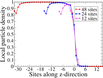
Figure 1: Comparison among density profiles corresponding to different sizes at $\lambda=0.5$ and $\epsilon=0.01t$. The index $0$ indicates the interface $Mn$-plane between the last $La$-plane in $LMO$ block and the first $Sr$-plane in $SMO$ block.

At first, we have analyzed the scaling of the static properties as function of the size of the system along the $z$ growth direction. Therefore, a comparison of the density profiles has been done with $(LMO)_{8}/(SMO)_{4}$, $(LMO)_{16}/(SMO)_{8}$ and $(LMO)_{32}/(SMO)_{16}$ systems. In Fig. 1, we show the density profiles in a situation where strain-induced anisotropy has not been introduced. It is worth noticing that we indicate the interface $Mn$-plane between the last $La$-plane in $LMO$ block and the first $Sr$-plane in $SMO$ block with the index $0$. For a sufficiently large numbers of planes, the charge profile along $z$ shows a well-defined shape. Indeed, the local density is nearly unity in $LMO$ block, nearly zero in $SMO$ block, and it decreases from $1$ to $0$ in the interface region. The decrease of charge density for the first planes of $LMO$ is due to the effect of open boundary conditions along the $z$ direction. In the intermediate electron-phonon coupling regime that we consider in Fig. (1), the region with charge dropping involves $4-5$ planes between the two blocks. We notice that the local charge density for $(LMO)_{16}/(SMO)_{8}$ and $(LMO)_{32}/(SMO)_{16}$ systems are very similar around the interface. Furthermore, the numerical results show close values of variational free energy corresponding to above mentioned systems. Given the similarity of the properties of these two systems, in the following, we will develop the analysis on the role of interface studying the system $(LMO)_{16}/(SMO)_{8}$.

For the same set of electron-phonon and magnetic couplings, the variational parameters and the Hartree self-consistent potential along z-axis are shown in Fig. 2. The effective magnetic fields are plotted for the most stable magnetic solution: antiferro $G$ orders well inside $LMO$ (planes $1-15$) and $SMO$ (planes $19-24$), and ferromagnetic planes at the interface (planes $16-18$). The peak in the plot of the magnetic fields signals that ferromagnetism is quite robust at the interface. The variational electron-phonon parameters $f_{i_{z}}$ are small on the $LMO$ side and at the interface, but close to unity in $SMO$ block. This means that, for these values of the couplings, carriers are delocalized in $LMO$ up to the interface region, but small polarons are present in the $SMO$ block. The quantities $\Delta_{i_{z}}$, entering the variational treatment of the electron-phonon coupling, are determined by $f_{i_{z}}$ and the local density $<n_{i_{z}}>$ through the equation: $\Delta_{i_{z}}=<n_{i_{z}}>(1-f_{i_{z}})$. The Hartree self-consistent potential $\Phi$ indicates that charges are trapped into a potential well corresponding to the $LMO$ block. Moreover, it is important to stress the energy scales involved in the well: the barrier between $LMO$ and $SMO$ block is of the order of the electron band-width. Furthermore, at the interface, the energy difference between neighboring planes is of the order of the hopping energy $t$.

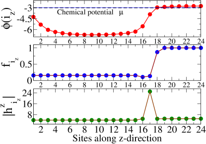
Figure 2: Self-consistent Hartree potential $\phi(i_{z})$ (upper panel, in units of $t$), variational parameters $f_{i_{z}}$ (mid panel) and effective magnetic fields $|h^{z}_{i_{z}}|$ (lower panel) along the z-axis for $\lambda=0.5$ and $\epsilon=0.01t$.

As mentioned above, for these systems, strain plays an important role. In order to study quantitatively its effect, we have investigated the phase diagram under the variation of the hopping anisotropy $t_{z}/t$ for two different values of $\epsilon_{z}$ ($\epsilon_{z}=\epsilon=0.01t$, $\epsilon_{z}=0$). Indeed, we simulate the compressive strain in the $LMO$ block increasing the ratio $t_{z}/t$ and decreasing $\epsilon_{z}/\epsilon$. On the other hand, the tensile strain in the $SMO$ block favour the more isotropic $x^{2}-y^{2}$ orbital and does not yield sizable effects. Therefore, for the $SMO$ block, in the following, we choose $t_{z}=t$ and $\epsilon_{z}=\epsilon$. For what concerns the electron-phonon interaction, we assume an intermediate coupling, $\lambda=0.8$. As shown in the upper panel of Fig. 3, with increasing the ratio $t_{z}/t$ up to $1.7$ for $\epsilon_{z}=\epsilon$, the magnetic order in $LMO$ does not change since it remains $G$ antiferromagnetic. However, the character of charge carriers is varied. Actually, for $\lambda=0.8$, in the absence of anisotropy, small polarons are present in the $LMO$ block. Moreover, at $t_{z}/t\simeq 1.5$, in $LMO$, a change from small localized polarons to large delocalized polaron occurs. For all values of the ratio $t_{z}/t$, the interface region is characterized by ferromagnetic order with large polaron carriers and $SMO$ by $G$ antiferromangnetic order with small polaron carriers.

Figure 3: Phase diagram in the hopping anisotropy-energy plane for $LMO_{16}SMO_{8}$ system, corresponding to $\lambda=0.8$ for $\epsilon_{z}=0.01t$ (upper panel) and $\epsilon_{z}=0$ (lower panel).

It has been shown that it is also important to consider the anisotropy in super-exchange ($\epsilon_{z}\neq\epsilon$) parameters as consequence of strain. fang In order to simulate the effect of compressive strain in $LMO$, a reduction of $\epsilon_{z}$ will be considered. We discuss the limiting case: $\epsilon_{z}=0$. For this regime of parameters, the effect on the magnetic phases is the strongest. As shown in the lower panel of Fig. 3, for $1.28\leq t_{z}/t\leq 1.5$, in $LMO$ block, a $C$-type antiferromagnetic phase is the most favorable. The transition from small to large polaron again takes place at $t_{z}/t\simeq 1.5$. Therefore, we have shown that there is a range of parameters where $LMO$ block has $C$-type antiferromagnetic order with small localized polarons. Due to the effect of strain, the magnetic solution in $LMO$ turns out to be compatible with experimental results in superlattices. aruta The interface is still ferromagnetic with metallic large polaron features. In the figure $A$/$B$/$C$ refers to magnetic orders and character of charge carriers inside $LMO$ (A), at interface (B), inside $SMO$ (C).

In order to analyze the effects of the electron-phonon interaction, a comparison between two different electron-phonon couplings is reported in Fig. 4. We have investigated the solutions which minimize the variational free energy at fixed value of the anisotropy factors $t_{z}/t=1.3$ and $\epsilon_{z}=0$ at $\lambda=0.5$ and $\lambda=0.8$. The magnetic solution in $LMO$ block is $C$ antiferromagnetic until the $15th$ plane. For both values of $\lambda$, polarons are small. In $SMO$ block, starting from the $19th$ plane, the solution is $G$-type antiferromagnetic together with localized polarons. Three planes around the interface are ferromagnetically ordered. For $\lambda=0.5$, all the three planes at the interface are characterized by delocalized polarons, while, for $\lambda=0.8$, only the plane linking the ends of $LMO$ and $SMO$ blocks is with delocalized charge carriers.

As shown in Fig. 4, the quantity $\lambda$ has important consequences on the physical properties such as the local particle density. Actually, for $\lambda=0.8$ the transition from occupied to empty planes is sharper at the interface. Only one plane at the interface shows an intermediate density close to $0.5$. For $\lambda=0.5$ the charge profile is smoother and the three ferromagnetic planes with large polarons have densities different from zero and one.

For the analysis of the spectral and optical quantities, we will consider the parameters used for the discussion of the results in this last figure.

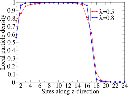
Figure 4: Comparison between local particle density corresponding to $\lambda=0.5$ and $\lambda=0.8$.

IV Spectral properties

In the following section we will calculate the spectral properties of the heterostructure for the same parameters used in Fig. 4.

Performing the canonical transformation (5) and exploiting the cyclic properties of the trace, the electron Matsubara Green’s function becomes

$$\mathcal{G}(\vec{R}_{i},\vec{R}_{j},\tau)=-\langle T_{\tau}c_{\vec{R}_{i}}(\tau)X_{\vec{R}_{i}}(\tau)c^{{\dagger}}_{\vec{R}_{j}}(0)X^{{\dagger}}_{\vec{R}_{j}}(0)\rangle.$$ (19)

By using the test Hamiltonian (7), the correlation function can be disentangled into electronic and phononic terms. perroni ; perroni1 Going to Matsubara frequencies and making the analytic continuation $i\omega_{n}\rightarrow\omega+i\delta$, one obtains the retarded Green’s function and the diagonal spectral function $A^{i_{x}i_{y}}_{i_{z}}(\omega)$ corresponding to $\vec{R}_{i}=\vec{R}_{j}$

$$A^{i_{x},i_{y}}_{i_{z}}(\omega)=$$

$$e^{S_{T}^{i_{z}}}\sum_{l=-\infty}^{\infty}I_{l}(S^{i_{z}})e^{\frac{\beta l\omega_{0}}{2}}[1-n_{F}(\omega-l\omega_{0})]g^{i_{x},i_{y}}_{i_{z}}(\omega-l\omega_{0})$$

$$+e^{S_{T}^{i_{z}}}\sum_{l=-\infty}^{\infty}I_{l}(S^{i_{z}})e^{\frac{\beta l\omega_{0}}{2}}n_{F}(\omega+l\omega_{0})g^{i_{x},i_{y}}_{i_{z}}(\omega+l\omega_{0}),$$

(20)

where $S^{i_{z}}_{T}=g^{2}f^{2}_{i_{z}}(2N_{0}+1)$, $S^{i_{z}}=2g^{2}f^{2}_{i_{z}}[N_{0}(N_{0}+1)]^{\frac{1}{2}}$, $I_{l}(z)$ modified Bessel functions, and $g^{i_{x},i_{y}}_{i_{z}}(\omega)$ is

$$g^{i_{x},i_{y}}_{i_{z}}(\omega)=\frac{2\pi}{N_{x}N_{y}}\sum_{\vec{k}_{||}}\sum_{n=1}^{2N_{z}}\delta[\omega-E(\vec{k}_{||},n)]$$

$$\times\Bigg{[}|b_{i_{z}}(\vec{k}_{||},n)|^{2}+|p_{i_{z}}(\vec{k}_{||},n)|^{2}+$$

$$(-1)^{i_{x}+i_{y}}[b^{*}_{i_{z}}(\vec{k}_{||},n)p_{i_{z}}(\vec{k}_{||},n)+p^{*}_{i_{z}}(\vec{k}_{||},n)b_{ic_{z}}(\vec{k}_{||},n)]\Bigg{]}.$$

The density of states $D(\omega)$ is defined as

$$D(\omega)=\frac{1}{N_{x}N_{y}N_{z}}\frac{1}{2\pi}\sum_{i_{x},i_{y},i_{z}}A^{i_{x},i_{y}}_{i_{z}}(\omega).$$ (22)

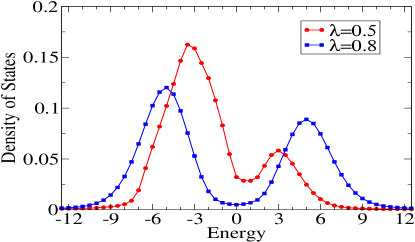
Figure 5: Comparison between density of states (in units of $1/t$) as a function of the energy (in units of $t$) corresponding to $\lambda=0.5$ and $\lambda=0.8$.

In Fig. 5 we report the density of state of the system $(LMO)_{16}/(SMO)_{8}$. It has been calculated measuring the energy to the chemical potential $\mu$. This comparison has been made at fixed low temperature ($K_{B}T=0.05t$), therefore we can consider the chemical potential very close to the Fermi energy of the system. At $\lambda=0.5$, the spectral function exhibits a residual spectral weight at $\mu$. The main contribution to the density of states at the chemical potential $\mu$ comes from the three ferromagnetic large polaron planes at the interface. Indeed, the contributions due to the ($LMO$) and ($SMO$) blocks is negligible.

For stronger electron-phonon coupling at $\lambda=0.8$, we observe an important depression of the spectral function at $\mu$. Hence the formation of a clear pseudogap takes place. This result is still compatible with the solution of our variational calculation since, for this value of $\lambda=0.8$, there is only one plane with delocalized charge carriers which corresponds to the plane indicated as the interface ($i_{z}=17$), while the two further ferromagnetic planes around the interface are characterized by small polarons. The depression of the density of the states at the Fermi energy is due also to the polaronic localization well inside the $LMO$ and $SMO$ block. In any case we find that, even for $\lambda=0.8$, the density of states never vanishes at the interface in agreement with experimental results. eckstein1

In this section we have found strong indications that a metallic ferromagnetic interface can form at the interface between $LMO$ and $SMO$ blocks. This situation should be relevant for superlattices with $n\geq 3$, where resistivity measurements made with contacts on top of $LMO$ show a globally insulating behavior. In our analysis we have completely neglected any effect due to disorder even if, both from experiments eckstein ; adamo1 and theories dagotto1 , it has been suggested that localization induced by disorder could be the cause of the metal-insulator transition observed for $n\geq 3$. We point out that the sizable source of disorder due to the random doping with $Sr^{2+}$ is strongly reduced since, in superlattices, $La^{3+}$ and $Sr^{2+}$ ions are spatially separated by interfaces. Therefore, the amount of disorder present in the heterostructure is strongly reduced in comparison with the alloy. However, considering the behavior of the $LMO$ ($SMO$) block as that of a bulk with a small amount of holes (particles), one expects that even a weak disorder induces localization. On the other hand, a weak disorder is not able to prevent the formation of the ferromagnetic metallic interface favored by the double-exchange mechanism and the charge transfer between the bulk-like blocks: the states at the Fermi level due to the interface formation have enough density eckstein1 so that they cannot be easily localized by weak disorder. In this section, we have shown that this can be the case in the intermediate electron-phonon coupling regime appropriate for $LMO/SMO$ heterostructures.

In the next section we will analyze the effects of electron-phonon coupling and strain on the optical conductivity in the same regime of the parameters considered in this section.

V Optical properties

To determine the linear response to an external field of frequency $\omega$, we derive the conductivity tensor $\sigma_{\alpha,\beta}$ by means of the Kubo formula. In order to calculate the absorption, we need only the real part of the conductivity

$$Re\sigma_{\alpha,\alpha}(\omega)=-\frac{Im\Pi^{ret}_{\alpha,\alpha}}{\omega},$$ (23)

where $\Pi^{ret}_{\alpha,\beta}$ is the retarded current-current correlation function. Following a well defined scheme perroni ; perroni1 and neglecting vertex corrections, one can get a compact expression for the real part of the conductivity $\sigma_{\alpha,\alpha}$. It is possible to get the conductivity both along the plane perpendicular to growth axis, $\sigma_{xx}$, and parallel to it, $\sigma_{zz}$. In order to calculate the current-current correlation function, one can use the spectral function $A_{\vec{k}_{||};i_{z},j_{z}}$ derived in the previous section exploiting the translational invariance along in-plane direction. It is possible to show that the components of the real part of the conductivity become

$$Re[\sigma_{xx}](\omega)=\frac{e^{2}t^{2}}{N_{x}N_{y}}\sum_{k_{x},k_{y}}4sen^{2}(k_{x})\frac{1}{N_{z}}\sum_{i_{z},j_{z}}\gamma_{i_{z}}\gamma_{j_{z}}$$

$$\times\frac{1}{\omega}\int^{\infty}_{-\infty}\frac{d\omega_{1}}{4\pi}[n_{F}(\omega_{1}-\omega)-n_{F}(\omega_{1})]$$

$$\times A_{k_{x},k_{y};i_{z},j_{z}}(\omega_{1}-\omega)A_{k_{x},k_{y};i_{z},j_{z}}(\omega_{1}),$$ (24)

and

$$Re[\sigma_{zz}](\omega)=\frac{e^{2}t^{2}}{N_{x}N_{y}}\sum_{k_{x},k_{y}}\frac{1}{N_{z}}\sum_{i_{z},j_{z}}\sum_{\delta_{1z},\delta_{2z}}\delta_{1z}\delta_{2z}$$

$$\times\eta_{i_{z},i_{z}+\delta_{1z}}\eta_{j_{z},j_{z}+\delta_{2z}}\frac{1}{\omega}\int^{\infty}_{-\infty}\frac{d\omega_{1}}{4\pi}[n_{F}(\omega_{1}-\omega)-n_{F}(\omega_{1})]$$

$$\times A_{k_{x},k_{y};i_{z}+\delta_{1z},j_{z}+\delta_{2z}}(\omega_{1}-\omega)A_{k_{x},k_{y};i_{z},j_{z}}(\omega_{1}).$$ (25)

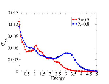
Figure 6: The conductivity (in units of $e^{2}/(mt)$, with $m=1/(2t)$) into the plane perpendicular to growth direction of the $(LMO)_{16}/(SMO)_{8}$ bilayer as a function of the energy (in units of $t$) for different values of $\lambda$.

In Fig. 6, we report the in-plane conductivity as function of the frequency at $\lambda=0.5$ and $\lambda=0.8$. We have checked that the in-plane response mainly comes from the interface planes. Both conductivities are characterized by a Drude-like response at low frequency. Therefore, the in-plane conductivity provides a clear signature of the formation of the metallic ferromagnetic interface. However, due to the effect of the interactions, we have found that the low frequency in-plane response is at least one order of magnitude smaller than that of free electrons in the heterostructures. Moreover, additional structures are present in the absorption with increasing energy. For $\lambda=0.5$, a new band with a peak energy of the order of hopping $t=2\omega_{0}$ is clear in the spectra. This structure can be surely ascribed to the presence of large polarons at the three interface planes. perroni Actually, this band comes from the incoherent multiphonon absorption of large polarons at the interface. This is also confirmed by the fact that this band is quite broad, therefore it can be interpreted in terms of multiple excitations. For $\lambda=0.8$, the band is even larger and shifted at higher energies. In this case, at the interface, large and small polarons are present with a ferromagnetic spin order. Therefore, there is a mixing of excitations whose net effect is the transfer of spectral weight at higher frequencies.

The out-of-plane optical conductivities show significant differences in comparison with the in-plane responses. In Fig. 7, we report out-of-plane conductivity as function of the frequency at $\lambda=0.5$ and $\lambda=0.8$. First, we observe the absence of the Drude term. Moreover, the band at energy about $2\omega_{0}$ is narrower than that in the in-plane response. Therefore, the origin of this band has to be different. Actually, the out-of-plane optical conductivities are sensitive to the interface region. A charge carrier at the interface has to overcome an energy barrier in order to hop to the neighbour empty site. As shown in Fig. 2, the typical energy for close planes at the interface is of the order of the hopping $t$. Therefore, when one electrons hops along $z$, it has to pay at least an energy of the order of $t$. In the out-of-plane spectra, the peaks at low energy can be ascribed to this process. Of course, by paying a larger energy, the electron can hop to next nearest neighbors. This explains the width of this band due to inter-plane hopping.

Additional structures are present at higher energies in the out-of-plane conductivities. For $\lambda=0.5$ the band at high energy is broad with small spectral weight. For $\lambda=0.8$, there is an actual transfer of spectral weight at higher energies. A clear band is peaked around $10t$. This energy scale can be intepreted as given by $2g^{2}\omega_{0}=9.6t$ for $\lambda=0.8$. Therefore, in the out-of-plane response, the contribution at high energy can be interpreted as due to small polarons. perroni ; mahan

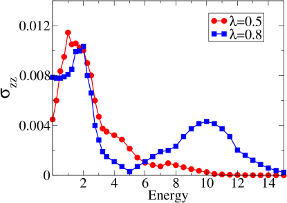
Figure 7: The conductivity (in units of $e^{2}/(mt)$, with $m=1/(2t)$) along the growth direction of the $(LMO)_{16}(SMO)_{8}$ bilayer as a function of the energy (in units of $t$) for $\lambda=0.5$ and $\lambda=0.8$.

Unfortunately, experimental data about optical properties of the $LMO/SMO$ bilayers are still not available. Therefore, comparison with experiments is not possible. Predictions about the different behaviors among $\sigma_{xx}$ and $\sigma_{zz}$ can be easily checked if one uses in-plane and out-of-plane polarization of the electrical fields used in the experimental probes. More important, the formation of two-dimensional gas at the interface expects to be confirmed by experiments made by using lateral contacts directly on the region between the $LMO$ and $SMO$ blocks. The d.c. conductivity of the sheet could directly measure the density of carriers of the interface metal and confirm the Drude-like low frequency behavior of in-plane response. Finally, one expects that a weak disorder present in the system and not included in our analysis can increase the scattering rate of the carriers reducing the value of the in-plane conductivity for $\omega\rightarrow 0$.

VI Conclusions

In this paper we have discussed phase diagrams, spectral and optical properties for a very large bilayer $(LMO)_{2n}/(SMO)_{n}$ (up to $48$ sites along the growth direction). A correlated inhomogeneous mean-field approach has been developed in order to analyze the effects of electron-lattice anti-adiabatic fluctuations and strain. We have shown that a metallic ferromagnetic interface is a quite robust feature of these systems for a large range of the electron-lattice couplings and strain strengths. Furthermore, we have found that the size of the interface region depends on the strength of electron-phonon interactions. At low temperature, the general structure of our solutions is characterized by three phases running along growth $z$-direction: antiferromagnetic phase with localized/Delocalized charge carriers inside $LMO$ block, ferromagnetic state with itinerant carriers at the interface, localized polaronic $G$-type antiferromagnetic phase inside $SMO$ block. The type of antiferromagnetic order inside $LMO$ depends on the strain induced by the substrate.

Spectral and optical properties have been discussed for different parameter regimes. Due to the formation of the metallic interface, even in the intermediate to strong electron-phonon coupling regime, the density of states never vanishes at the chemical potential. Finally, in-plane and out-of-plane optical conductivities are sharply different: the former shows a metallic behavior, the latter a transfer of spectral weight at high frequency due to the effects of the electrostatic potential well trapping electrons in $LMO$ block. The in-plane response provides a signature of the formation of the metallic ferromagnetic interface.

In this paper we have focused on static and dynamic properties at very low temperature. The approach used in the paper is valid at any temperature. Therefore, it could be very interesting to analyze not only single interfaces, but also superlattices with different unit cells at finite temperature. Work in this direction is in progress.

Appendix A

In this Appendix we give some details about the effective electronic Hamiltonian derived within our approach. After the Hartree approximation for the long-range Coulomnb interactions, the mean-field electronic Hamiltonian reads:

$$H^{el}_{test}=-t\sum_{i_{||}}\sum_{i_{z}=1}^{N_{z}}\sum_{\delta_{||}}\gamma_{i_{z}}e^{-V_{i_{z}}}c^{{\dagger}}_{i_{||},i_{z}}c_{i_{||}+\delta_{||},i_{z}}$$

$$-t\sum_{i_{||}}\sum_{i_{z}=1}^{N_{z}}\sum_{\delta_{z}}\eta_{i_{z},i_{z}+\delta_{z}}e^{-W_{i_{z},i_{z}+\delta_{z}}}c^{{\dagger}}_{i_{||},i_{z}}c_{i_{||},i_{z}+\delta_{z}}$$

$$+\sum_{i_{||}}\sum_{i_{z}=1}^{N_{z}}[\phi(i_{z})-\mu]c^{{\dagger}}_{i_{||},i_{z}}c_{i_{||},i_{z}}+N_{x}N_{y}(T_{1}+T_{2})$$

$$+N_{x}N_{y}g^{2}\omega_{0}\sum_{i_{z}}\Delta_{i_{z}}+\sum_{i_{||}}\sum_{i_{z}=1}^{N_{z}}C_{i_{z}}(g^{2}\omega_{0})c^{{\dagger}}_{i_{||},i_{z}}c_{i_{||},i_{z}}.$$ (26)

The self-consistent Hartee potential is given by

$$\phi(i_{z})=\frac{e^{2}}{\epsilon}[\sum_{j_{z}>i_{z}}\chi(j_{z})S(i_{z}-j_{z})+$$

$$\sum_{j_{z}<i_{z}}\chi(j_{z})S(i_{z}-j_{z})+S_{1}(0)\chi(i_{z})-S_{2}(i_{z})],$$ (27)

where the quantity $T_{1}$ is

$$T_{1}=\frac{-e^{2}}{2\epsilon}[\sum_{i_{z}=1}^{N_{z}}\sum_{j_{z}>i_{z}}^{N_{z}}\chi_{i_{z}}\chi_{j_{z}}S(i_{z}-j_{z})+$$

$$\sum_{j_{z}<i_{z}}^{N_{z}}\chi_{i_{z}}\chi_{j_{z}}S(i_{z}-j_{z})+S_{1}(0)\sum_{i_{z}}^{N_{z}}\chi_{i_{z}}^{2}],$$ (28)

and $T_{2}$

$$T_{2}=\frac{e^{2}}{2\epsilon}[\sum_{I_{z}=1}^{N_{La}}\sum_{J_{z}>I_{z}}^{N_{La}}S(I_{z}-J_{z})+$$

$$\sum_{J_{z}<I_{z}}^{N_{La}}S(I_{z}-J_{z})+N_{La}S_{1}]$$ (29)

with $S(n_{z})$, $S_{1}(0)$ end $S_{2}(n_{z})$ obtained by adding the Coulomb terms on in-plane lattice index. The summations have been made modulating the Coulomb interaction with a screening factor: $\frac{e^{2}}{|\vec{r}_{i}-\vec{r}_{j}|}\rightarrow\frac{e^{2}e^{-\eta_{S}|\vec{r}_{i}-\vec{r}_{j}|}}{|\vec{r}_{i}-\vec{r}_{j}|}$, where $\frac{1}{\eta_{S}}$ is a fictitious finite screening length in units of the lattice parameter $a$. Therefore, $S(n_{z})$ is

$$S(n_{z})=\sum_{m_{x},m_{y}}\frac{\exp{\left(-\eta_{S}\sqrt{m^{2}_{x}+m^{2}_{y}+n^{2}_{z}}\right)}}{\sqrt{m^{2}_{x}+m^{2}_{y}+n^{2}_{z}}},$$ (30)

$S_{1}(0)$ is given by

$$S_{1}(0)=\sum_{m_{x},m_{y}}\frac{\exp{\left(-\eta_{S}\sqrt{m^{2}_{x}+m^{2}_{y}}\right)}}{\sqrt{m^{2}_{x}+m^{2}_{y}}},$$ (31)

with $(m_{x},m_{y})\neq(0,0)$, and $S_{2}(i_{z}-j_{z})$ is

$$S_{2}(n_{z})=\sum_{m_{x},m_{y}}\sum_{i_{z}=1}^{l_{z}}\frac{\exp{\left(-\eta_{S}\sqrt{h_{x}^{2}+h_{y}^{2}+h_{z}^{2}}\right)}}{\sqrt{h_{x}^{2}+h_{y}^{2}+h_{z}^{2}}},$$ (32)

with $l_{z}$ number of the planes of $LMO$ block, $h_{x}=m_{x}-0.5$, $h_{y}=m_{y}-0.5$, and $h_{z}=n_{z}-i_{z}-0.5$.

References

References

- (1) M. Imada, A. Fujimori, and Y. Tokura, Rev. Mod. Phys. 70, 1039 (1998).
- (2) E. Dagotto, Nanoscale Phase Separation and Colossal Magnetoresistance (Springer-Verlag, Heidelberg, 2003).
- (3) C. Zener, Phys. Rev. 81, 440 (1951); C. Zener, ibid. 82, 403 (1951); P.W. Anderson and H. Hasegawa, ibid. 100, 675 (1955); P.G. de Gennes, ibid. 118, 141 (1960).
- (4) A.J. Millis, Nature (London) 392, 147 (1998).
- (5) A. Ohtomo and H. Y. Hwang, Nature (London) 419, 378 (2002); S. Okamoto and A. J. Millis, Nature (London) 428, 630 (2004).
- (6) A. Ohtomo and H. Y. Hwang, Nature (London) 427, 423 (2004) ; S. Thiel, G. Hammerl, A. Schmehl, C. W. Schneider, and J. Mannhart, Science 313, 1942 (2006); N. Reyren , ibid. 317, 1196 (2007).
- (7) T. Koida, M. Lippmaa, T. Fukumura, K. Itaka, Y. Matsumoto, M. Kawasaki, and H. Koinuma, Phys. Rev. B 66, 144418 (2002); H. Yamada, M. Kawasaki, T. Lottermoser, T. Arima, and Y. Tokura, Appl. Phys. Lett. 89, 052506 (2006).
- (8) A. Bhattacharya, S.J. May, S.G.E. Velthuis, M. Warusawithana, X. Zhai, B. Jiang, J.M. Zuo, M.R. Fitzsimmons, S.D. Bader, and J.N. Eckstein, Phys. Rev. Lett. 100, 257203 (2008).
- (9) C. Adamo, X. Ke, P. Schiffer, A. Soukiassian, M. Warusawithana, L. Maritato, and D.G. Schlom, Appl. Phys. Lett. 92, 112508 (2008).
- (10) C. Adamo, C. A. Perroni, V. Cataudella, G. De Filippis, P. Orgiani, and L. Maritato, Phys. Rev. B 79, 045125 (2009).
- (11) N. Ogawa, T. Satoh, Y. Ogimoto, and K. Miyano, Phys. Rev. B 78, 212409 (2008).
- (12) S. Smadici, P. Abbamonte, A. Bhattacharya, X. Zhai, B. Jiang, A. Rusydi, J.N. Eckstein, S.D. Bader, and J.-M. Zuo, Phys. Rev. Lett. 99, 196404 (2007).
- (13) N. Ogawa, T. Satoh, Y. Ogimoto, and K. Miyano, Phys. Rev. B 80, 241104(R) (2009).
- (14) B.R.K. Nanda and S. Satpathy, Phys. Rev. Lett. 101, 127201 (2008); B.R.K. Nanda and S. Satpathy, Phys. Rev. B 79, 054428 (2009).
- (15) C. Aruta, C. Adamo, A. Galdi, P. Orgiani, V. Bisogni, N. B. Brookes, J.C. Cezar, P. Thakur, C.A. Perroni, G. De Filippis, V. Cataudella, D.G. Schlom, L. Maritato, and G. Ghiringhelli, Phys. Rev. B 80, 140405(R) (2009).
- (16) H. Yamada, P.H. Xiang, and A. Sawa, Phys. Rev. B 81, 014410 (2010).
- (17) S. Dong, R. Yu, S. Yunoki, G. Alvarez, J.-M. Liu ,and E. Dagotto, Phys. Rev. B 78, 201102(R) (2008); R. Yu, S. Yunoki, S. Dong, and E. Dagotto, Phys. Rev. B 80, 125115 (2009).
- (18) C. Lin and A.J. Millis, Phys. Rev. B 78, 184405 (2008).
- (19) C. Lin, S. Okamoto, and A.J. Millis, Phys. Rev. B 73, 041104(R) (2006).
- (20) B.R.K. Nanda and S. Satpathy, Phys. Rev. B 78, 054427 (2008); B.R.K. Nanda and S. Satpathy, Phys. Rev. B 81, 224408 (2010).
- (21) Shuai Dong, Seiji Yunoki, Xiaotian Zhang, Cengiz Sen, J.-M. Liu, and Elbio Dagotto, arXiv:1005.3865 (2010).
- (22) Z. Fang, I. V. Solovyev, and K. Terakura, Phys. Rev. Lett. 84, 3169 (2000).
- (23) C.A. Perroni, G. De Filippis, V. Cataudella, and G. Iadonisi, Phys. Rev. B 64, 144302 (2001).
- (24) C.A. Perroni, V. Cataudella, G. De Filippis, G. Iadonisi, V. Marigliano Ramaglia, and F. Ventriglia, Phys. Rev. B 68, 224424 (2003).
- (25) A. Iorio, C. A. Perroni, G. De Filippis, V. Marigliano Ramaglia, V. Cataudella, J. Phys.: Condens. Matter 21, 456002 (2009).
- (26) I.J. Lang and Yu. A. Firsov, Sov. Phys. JETP 16, 1301 (1963).
- (27) G. Mahan, Many-Particle Physics, 2nd ed. (Plenum Press, New York, 1990).