On fair pricing of emission-related derivatives

Abstract

Tackling climate change is at the top of many agendas. In this context, emission trading schemes are considered as promising tools. The regulatory framework for an emission trading scheme introduces a market for emission allowances and creates a need for risk management by appropriate financial contracts. In this work, we address logical principles underlying their valuation.

and

1 Introduction

The generic principle of an emission trading scheme is based on the so-called ‘cap-and-trade’ mechanism. In this framework, an authority allocates fully tradable credits among responsible institutions. At pre-settled compliance dates, each source must have enough allowances to cover all of its recorded emissions, or be subject to penalties.

A mandatory cap-and-trade system involves its participants in a risky business with an obvious need for risk management. That is, certificate trading is usually accompanied by a secondary market for emission-related futures, including a rapidly growing variety of their derivatives. Their pricing is addressed in this work.

Our contribution focuses on a methodology between equilibrium and risk-neutral approaches. Due to the complexity of emissions markets, risk-neutral dynamics must be addressed in terms of explanatory variables, viewed as proxies of fundamental quantities. Thus, we utilize equilibrium analysis to explain the role of fundamentals in risk-neutral allowance price formation. Thereby, the key issue is a feedback relation between allowance prices and abatement activity. Namely, we demonstrate that any increase in allowance price causes market participants to enforce emission saving in order to sell their allowances. Hence, an increasing allowance price encourages a supply of certificates and lowers the probability of non-compliance, which tends to bring down their prices. Apparently, the correct description of this feedback is the key to derivatives pricing. The present work focuses on this issue. On this account, our contribution goes beyond any risk-neutral approach to modeling of emission-related assets suggested in the existing literature to date.

2 Emissions markets

The literature on this subject is enormous: it encompass hundreds of books and papers. For this reason, we focus only on those market models which are relevant in the present approach.

Economic theory of allowance trading can be traced back to [8] and [14], whose authors proposed a market model for the public environmental goods described by tradable permits.

Dynamic allowance trading is addressed in [7, 22, 16, 11, 17, 21, 13] and in the literature cited therein.

Empirical evidence from existing markets is discussed in [9]. This paper suggests economic implications and hints at several ways to model spot and futures allowance prices, whose detailed interrelations are investigated in [23] and [24].

Econometric modeling is addressed in [1], where characteristic properties for financial time series are observed for prices of emission allowances from the mandatory European Scheme EU ETS. Furthermore, a Markov switch and AR–GARCH models are suggested. The work [15] also considers tail behavior and the heteroscedastic dynamics in the returns of emission allowance prices.

Dynamic price equilibrium and optimal market design are investigated in [2]. Based on this approach, [3] discusses the price formation for goods whose production is affected by emission regulations. In this setting, an equilibrium analysis confirms the existence of the so-called ‘windfall profits’ (see [19]) and provides quantitative tools to analyze alternative market designs.

Pricing of options was addressed only recently. The paper [6] discusses an endogenous emission permit price dynamics within equilibrium setting and elaborates on valuation of European option on emission allowances. The paper [18] and the dissertation [25] deal with the the risk-neutral allowance price formation within EU ETS. Here, utilizing equilibrium properties, the price evolution is treated in terms of marginal abatement costs and optimal stochastic control. Also, the work [5] is devoted to option pricing within EU ETS. The authors suppose that the drift of allowance spot prices is related to a hidden variable which describes the overall market position in allowance contracts and they make use of filtering techniques to derive option price formulas which reflect specific allowance banking regulations, valid in the EU ETS. Finally, the recent work [4] presents an approach where emission certificate futures are modeled in terms of deterministic time change applied to a certain class of interval-valued diffusion processes.

The present work brings aspects of risk-aversion into the line of research followed in [18, 3] and [2], which we briefly sketch now. Within a stochastic model of an emissions market, a so-called central planer problem is introduced and discussed in [18]. Under additional assumptions, the authors formulate this problem in terms of continuous-time stochastic optimization. Furthermore, they provide economic arguments justifying why optimal control solutions correspond to an equilibrium of the emissions market. Interpreting the allowance certificate price as the marginal abatement costs, particular explicit solutions are discussed and yield a dynamic stochastic model for allowance price evolution. The work [2] starts from the opposite direction. In a discrete-time framework, the Radner equilibrium of an emissions market is introduced and constructed via a solution of the central planer problem. The work [3] yields an extension: in a slightly different setting, it is proved that any market equilibrium is reached by this methodology. Thus, results from [18, 2] and [3] show that a quantitative analysis of emissions markets is tractable in terms of stochastic control theory. However, this connection is valid only if risk aversion is neglected, in other words, under the assumption that each agent possesses a linear utility function. Losing sight of risk aversion comes at the costs of unrealistic results. Among other singularities, it turns out that the equilibrium allowance price follows a martingale (with respect to objective measure!) with the consequence that allowance trading can be arbitrary, only the final position must be adjusted accordingly.

This work resolves all of these problems. Starting from the no-arbitrage property which is satisfied in an equilibrium of a market with risk-averse players, we show that the risk-neutral allowance price dynamics exhibits the above feedback property, which we formalize as a fixed point equation, discussing its solution. We show that for such a risk-averse setting, our fixed point equation plays the same role as the central planer optimal control problem for the non-risk-averse situation. Namely, it provides a methodology to describe the market equilibrium in terms of aggregated quantities. However, this description is valid only from the viewpoint of the so-called risk neutral dynamics, not being suitable for discussing all interesting problems. Still, derivatives valuation is naturally addressed in, and can be obtained in, this setting.

3 Mathematical model

Let $(\Omega,{\cal F},{\mathrm{P}},({\cal F}_{t})_{t=0}^{T})$ be a filtered probability space. Assume that ${\cal F}_{0}$ is deterministic and agree that all processes considered in this work are adapted to $({\cal F}_{t})_{t=0}^{T}$. Write $\mathbb{E}_{t}(\cdot)$ and ${\mathrm{P}}_{t}$ to denote, respectively, conditional expectation and conditional distribution with respect to ${\cal F}_{t}$. Consider a market with a finite number $I$ of the agents confronted with emission reduction.

Emission dynamics. For each agent $i\in I$, introduce the stochastic process $(E^{i}_{t})_{t=0}^{T-1}$ with the interpretation that $E^{i}_{t}$ describes the total pollution of the agent $i$ which is emitted within the time interval $[t,t+1]$ in the case of the so-called ‘business-as-usual’ scenario (where no abatement measure is applied). Although each agent is considered as a potential producer, purely financial institutions are also covered with this approach by setting emissions to zero, that is, $E^{i}_{t}=0$ for $t=0,\ldots,T-1$.

Abatement. Consider the opportunity to reduce emissions. Each agent $i$ can decide at any time $t=0,\ldots,T-1$ to reduce its emissions within $[t,t+1]$ by $\xi^{i}_{t}$ pollutant units. We suppose that each abatement level is possible, ranging from no reduction to full reduction. Hence, we assume that $0\leq\xi^{i}_{t}\leq E^{i}_{t}$ holds for all $t=0,\ldots,T-1$.

Abatement costs. We assume that the cost of abatement is a random function of the reduced volume. The randomness is due to uncertainty in prices (of fuel) and is observable at the corresponding time. Thus, if the agent $i$ decides at time $t=0,\ldots,T-1$ on reduction of their own emissions by $x\in[0,\infty[$ units, then it causes costs $C^{i}_{t}(x)$, where given

$$\cases{C^{i}_{t}\mathchoice{\nobreak\,\colon}{\nobreak\,\colon}{\nobreak\,\colon\;}{\nobreak\,\colon\;}[0,\infty[\times\Omega\mapsto\mathbb{R}\mbox{ is }{\cal B}([0,\infty[)\otimes{\cal F}_{t}\mbox{-measurable}\cr\mbox{and for each }\omega\in\Omega,x\mapsto C^{i}_{t}(x)(\omega)\mbox{ is strictly}\cr\mbox{convex and continuous with }C(0)=0.}$$ (1)

Since emission savings cannot exceed the business-as-usual emission, the abatement activity $(\xi^{i}_{t})_{t=0}^{T-1}$ is feasible if

$$0\leq\xi^{i}_{t}\leq E^{i}_{t},\qquad t=0,\ldots,T-1.$$ (2)

Following abatement policy $(\xi^{i}_{t})_{t=0}^{T-1}$, the agent $i$ accumulates at the compliance date $T$ the total terminal costs

$$\sum_{t=0}^{T-1}C^{i}_{t}(\xi^{i}_{t}).$$ (3)

Abatement volume. For later use, let us introduce, for each $\omega\in\Omega$, $t=0,\ldots,T-1$ and $a\in[0,\infty[$, the abatement volume $c_{t}^{i}(a)(\omega)$ as

$$c_{t}^{i}(a)(\omega):=\arg\min\{C_{t}^{i}(x)(\omega)-ax\mathchoice{\nobreak\,\colon}{\nobreak\,\colon}{\nobreak\,\colon\;}{\nobreak\,\colon\;}x\in[0,E^{i}_{t}(\omega)]\},$$ (4)

which is well defined since, under the assumptions (1), the minimum of the function $x\mapsto C_{t}^{i}(x)(\omega)-ax$ on $[0,E^{i}_{t}(\omega)]$ is attained at the unique point. The reader may imagine $c_{t}^{i}(a)(\omega)$ as the total reduction volume which is available within $[t,t+1]$ in the situation $\omega$ at a price which is less than or equal to $a$ (measured in currency unit per pollutant unit). A straightforward proof shows that (1) ensures that

$$[0,\infty[\mapsto\mathbb{R},a\mapsto c_{t}^{i}(a)(\omega)\mbox{ is non-decreasing and}$$

(5)

$$\mbox{continuous for almost every }\omega\in\Omega\mbox{ and }t=0,\ldots,T-1.$$

For later use, we introduce the cumulative abatement volume function

$$c_{t}(a):=\sum_{i\in I}c^{i}_{t}(a),\qquad a\in[0,\infty[.$$ (6)

Obviously, $c_{t}(a)(\omega)$ stands for the total abatement in the market, which is available from all measures in the situation $\omega$ whose price is less than or equal to $a\in[0,\infty[$.

Allowance trading. Suppose that, at any time $t=0,\ldots,T$, credits can be exchanged between agents by trading at the spot price $A_{t}$. Denote by $\vartheta^{i}_{t}$ the change at time $t$ in allowance number held by agent $i$. That is, given the allowance prices $(A_{t})_{t=0}^{T}$, the position changes $(\vartheta^{i}_{t})_{t=0}^{T}$ yield costs

$$\sum_{t=0}^{T}\vartheta^{i}_{t}A_{t}.$$ (7)

Penalty payment. The total pollution of the agent $i$ can be expressed as a difference

$$\sum_{t=0}^{T-1}E^{i}_{t}-\sum_{t=0}^{T-1}\xi^{i}_{t}$$

of the cumulative business-as-usual emission less the entire reduction. As mentioned above, a penalty $\pi\in]0,\infty[$ is being paid at maturity $T$ for each unit of pollutant, which is not covered by allowances. Considering the total change in the allowance position $\sum_{t=0}^{T}\vartheta^{i}_{t}$ effected by trading, the loss of the agent $i$ resulting from potential penalty payment is

$$\pi\Biggl{(}\sum_{t=0}^{T-1}(E^{i}_{t}-\xi^{i}_{t}-\vartheta^{i}_{t})-\gamma^{i}-\vartheta^{i}_{T}\Biggr{)}^{+},$$ (8)

where

$$\gamma^{i},\ i\in I\mbox{ are agents' initial allowance allocations}.$$ (9)

Remark 1.

Our stylized scheme deals with stand-alone emission trading mechanisms. In the real world, cap-and-trade systems operate on multi-period scales, where unused allowances can be carried out (banked) into next period. Further period interconnections may include a transfer of future allocation from the next into the present period (borrowing) and, in the case of non-compliance, a withdrawal of an appropriate number of credits from the next period allocation in addition to penalty payment. To complete the complexity, let us mention that different emissions markets could be interconnected by acceptance of foreign certificates in the national scheme. Emission trading in multi-period settings is addressed in, among others, [4] and [5]. Mathematically, it reduces to the specification of a more complex penalty mechanism than that presented above. For this reason, we have decided to focus on the stand-alone allowance market to analyze quantitative methods in the simplest situation before tackling multi-scale systems (such as the second period of EU ETS).

Recording uncertainty. In what follows, we also need to take into account uncertainty in the emission recording. It is convenient to subtract these recording errors from the initial allocation. Hence, we interpret $\gamma^{i}$ as the credits allocated to the agent $i$ less emissions which become known with certainty only at time $T$. With this interpretation, $\gamma_{i}$ stands for allowances effectively available for compliance and is modeled by an ${\cal F}_{T}$-measurable random variable. For later use, let us agree that the distribution of $\sum_{i\in I}\gamma^{i}$, conditioned on ${\cal F}_{T-1}$, possesses almost surely no point masses, which implies that

$$P\biggl{(}\sum_{i\in I}\gamma^{i}=X\biggr{)}=0\qquad\mbox{for each ${\cal F}_{T-1}$-measurable $X$.}$$ (10)

Admissible policies. Since maximally possible reduction cannot exceed emission, wehave (2). Let us define the space of feasible trading $\vartheta^{i}=(\vartheta^{i}_{t})_{t=0}^{T}$ and abatement strategies $\xi^{i}=(\xi^{i}_{t})_{t=0}^{T-1}$ of the agent $i\in I$ by

$${\cal U}^{i}:=\{(\vartheta^{i},\xi^{i})\mathchoice{\nobreak\,\colon}{\nobreak\,\colon}{\nobreak\,\colon\;}{\nobreak\,\colon\;}0\leq\xi^{i}_{t}\leq E^{i}_{t},t=0,\ldots,T-1\}.$$ (11)

Individual wealth. In view of (3), (7) and (8), the revenue of the agent $i$ following admissible policy $(\vartheta^{i},\xi^{i})\in{\cal U}^{i}$ equals

$$L^{A,i}(\vartheta^{i},\xi^{i}) = -\sum_{t=0}^{T-1}\bigl{(}\vartheta^{i}_{t}A_{t}+C^{i}(\xi^{i}_{t})\bigr{)}$$

$${}-\vartheta^{i}_{T}A_{T}-\pi\Biggl{(}\sum_{t=0}^{T-1}(E^{i}_{t}-\xi^{i}_{t}-\vartheta^{i}_{t})-\gamma^{i}-\vartheta^{i}_{T}\Biggr{)}^{+}.$$

Risk aversion. To face risk preferences, suppose that attitudes of the agents $i\in I$ are described by utility functions $U^{i}\mathchoice{\nobreak\,\colon}{\nobreak\,\colon}{\nobreak\,\colon\;}{\nobreak\,\colon\;}\mathbb{R}\mapsto\mathbb{R},$ which are continuous, strictly increasing and concave. Consider the utility functional $u^{i}(X)=E(U^{i}(X)),$ which is assumed to be defined for each random variable $X$ where the expectation is finite or $+\infty$. Given allowance price process $A=(A_{t})_{t=0}^{T}$, the agent $i$ behaves rationally, maximizing $(\vartheta^{i},\xi^{i})\mapsto u^{i}(L^{A,i}(\vartheta^{i},\xi^{i}))$ by an appropriate choice of their own policy $(\vartheta^{i*},\xi^{i*})$.

Market equilibrium. Following standard theory, a realistic market state is described by the so-called equilibrium – a situation where the allowance price, positions and abatement measures are such that each agent is satisfied by their own policy and, at the same time, natural restrictions are fulfilled. In our framework, an appropriate notion of equilibrium is given as follows.

Definition 1.

The process $A^{*}=(A^{*}_{t})_{t=0}^{T}$ is called an equilibrium allowance price process if, for each $i\in I$, there exists $(\vartheta^{*i},\xi^{*i})\in{\cal U}^{i}$ such that $u^{i}(L^{A^{*},i}(\vartheta^{*i},\xi^{*i}))$ is finite and

1. [(ii)]

2. the cumulative changes in positions are in zero net supply, that is,

   $$\sum_{i\in I}\vartheta_{t}^{*i}=0\qquad\mbox{for all $t=0,\ldots,T$};$$ (13)

3. each agent $i\in I$ is satisfied by their own policy, in the sense that

   $$u^{i}(L^{A^{*},i}(\vartheta^{*i},\xi^{*i}))\geq u^{i}(L^{A^{*},i}(\vartheta^{i},\xi^{i}))$$

   (14)

   $$\quad\mbox{for each }(\vartheta^{i},\xi^{i})\in{\cal U}^{i}\mbox{ where }u^{i}(L^{A^{*},i}(\vartheta^{i},\xi^{i}))\mbox{ exists.}$$

The existence of emissions market equilibrium is addressed in [2] and [3], under the assumption of a linear utility function and in a slightly different setting. However, although equilibrium modeling in the spirit of these contributions is appropriate to investigate important questions of optimal market design, it has little to offer to the problem of derivatives valuation. With the present approach, we intend to establish a reduced-form model which describes the evolution of emission-related assets from a risk-neutral perspective. We obtain a realistic picture by incorporating three essential assumptions into a risk-neutral model. These assumptions are shown to be direct consequences of an equilibrium situation:

1. [(b)]

2. There is no arbitrage since, in equilibrium, any profitable strategy would immediately be followed by all agents. This would instantaneously change prices and exhaust any arbitrage opportunity.

3. The allowance trading instantaneously triggers all abatement measures whose costs are below allowance price. The explanation here is that if an agent possess a technology with lower reduction costs than the present allowance price, then it is optimal for that agent to immediately reduce pollution and take profit from selling allowances.

4. There are only two final outcomes for allowance price. Either the terminal allowance price drops to zero or it approaches the penalty level. The reason is that at maturity, the price must vanish if there is an excess in allowances, whereas in the case of their shortage, the price will rise, reaching penalty. We believe that in reality, an exact coincidence of allowance demand and supply occurs with zero probability and can be neglected.

Let us formalize the above assertions (a), (b) and (c).

Proposition 1.

Suppose that $(A^{*}_{t})_{t=0}^{T}$ is an equilibrium allowance price and $(\xi^{i*}_{t})_{t=0}^{T-1}$ for $i\in I$ are the corresponding equilibrium abatement policies.

1. [(b)]

2. There exists a measure $Q$ which is equivalent to $P$ such that $(A^{*}_{t})_{t=0}^{T}$ follows a $Q$-martingale.

3. For each $i\in I$, we have

   $$\xi^{i*}_{t}=c_{t}^{i}(A^{*}_{t}),\qquad t=0,\ldots,T-1,$$ (15)

   with abatement volume functions $c_{t}^{i}$, $t=0,\ldots,T-1$, from (4).

4. The terminal value of the allowance price is given by

   $$A^{*}_{T}=\pi 1_{\{\sum_{i\in I}(\sum_{t=0}^{T-1}(E^{i}_{t}-\xi^{i*}_{t})-\gamma^{i})\geq 0\}}.$$ (16)

Before we proceed with the proof, let us emphasize that this result can serve as a starting point for risk-neutral modeling. The above proposition states that at equilibrium, the allowance price process $(A^{*}_{t})_{t=0}^{T}$ follows a martingale with respect to an equivalent measure ${\mathrm{Q}}\sim{\mathrm{P}}$ whose terminal value is

$$A^{*}_{T}=\pi 1_{\{\sum_{i\in I}\sum_{t=0}^{T}(E^{i}_{t}-\xi^{*}_{t})-\gamma^{i})\geq 0\}},$$

obviously depending on intermediate values $(A^{*}_{t})_{t=0}^{T-1}$ through abatement volume function $\xi^{i*}_{t}=c^{i}_{t}(A^{*}_{t})$ for $t=0,\ldots,T-1,i\in I$. The surprising and far-reaching consequence is that, from a risk-neutral perspective, only cumulative market quantities are relevant. To see this, define the overall allowance shortage

$${\cal E}_{T}=\sum_{i\in I}\Biggl{(}\sum_{t=0}^{T-1}E^{i}_{t}-\gamma^{i}\Biggr{)}$$ (17)

which would appear in the market without any emission penalty. Further, recall from (4) and (6) the cumulative abatement functions to express the risk-neutral certificate price dynamics in terms of the following feedback equation:

$$A_{t}=\mathbb{E}^{Q}_{t}\bigl{(}\pi 1_{\{{\cal E}_{T}-\sum_{t=0}^{T-1}c_{t}(A^{*}_{t})\geq 0\}}\bigr{)},\qquad t=0,\ldots,T-1.$$

Although individual market attributes and actions of the different agents seem to be irrelevant in this picture, the reader should notice that this picture appears only from the risk-neutral viewpoint. In line with standard aggregation theorems, the equilibrium market state heavily depends on, and is determined by, market architecture, rules, risk attitudes and uncertainty. However, once equilibrium is reached and all arbitrage opportunities are exhausted, asset dynamics can be considered under risk-neutral measure. With respect to this measure, market evolution appears as if it were driven by cumulative quantities only.

With this in mind, let us formulate the problem of the reduced-form modeling as follows:

$$\cases{\mbox{Given measure }{\mathrm{Q}}\sim{\mathrm{P}},\mbox{ random variable }{\cal E}_{T}\cr\mbox{and abatement volume functions }(c_{t})_{t=0}^{T-1},\cr\mbox{determine a }{\mathrm{Q}}\mbox{-martingale }(A^{*}_{t})_{t=0}^{T}\mbox{ with}\cr A^{*}_{T}=\pi 1_{\{{\cal E}_{T}-\sum_{t=0}^{T-1}c_{t}(A^{*}_{t})\geq 0\}}.}$$ (18)

Note that this formulation serves as a guideline for martingale modeling since price-dependent abatement volume $c_{t}(a)$ can be estimated from market data, whereas potential allowance shortage ${\cal E}_{T}$ can be modeled in terms of total allowance allocation and demand fluctuations on goods whose production causes the pollution. Finally, we shall emphasize a natural passage to continuous time.

$$\cases{\mbox{Given, on a probability space }(\Omega,{\cal F},P,({\cal F}_{t})_{t\in[0,T]}),\cr\mbox{an equivalent measure }{\mathrm{Q}}\sim{\mathrm{P}},\mbox{ random variable }{\cal E}_{T}\cr\mbox{and a family of abatement functions }(c_{t})_{t\in[0,T]},\cr\mbox{determine a }{\mathrm{Q}}\mbox{-martingale }(A^{*}_{t})_{t\in[0,T]}\mbox{ with}\cr A^{*}_{T}=\pi 1_{\{{\cal E}_{T}-\int_{0}^{T}c_{t}(A^{*}_{t})\,\mathrm{d}t\geq 0\}}.}$$ (19)

Proof of Proposition 1 (a) According to the first fundamental theorem of asset pricing (see [10]), it suffices to verify that if $(A^{*}_{t})_{t=0}^{T}$ is an equilibrium allowance price process, then there is no arbitrage for allowance trading. Let us follow an indirect proof, supposing that $(\nu_{t})_{t=0}^{T-1}$ is an allowance trading arbitrage, meaning that

$${\mathrm{P}}\Biggl{(}\sum_{t=0}^{T-1}\nu_{t}(A_{t+1}-A_{t})\geq 0\Biggr{)}=1,\qquad{\mathrm{P}}\Biggl{(}\sum_{t=0}^{T-1}\nu_{t}(A_{t+1}-A_{t})>0\Biggr{)}>0.$$ (20)

Now, we verify that in the presence of arbitrage, no equilibrium can exist since each agent $i$ can change their own policy $(\vartheta^{*i},\xi^{*i})$ to an improved strategy $(\tilde{\vartheta}^{i},\xi^{*i})$ satisfying

$$u^{i}(L^{A^{*},i}(\vartheta^{*i},\xi^{*i}))<u^{i}(L^{A^{*},i}(\tilde{\vartheta}^{i},\xi^{*i})).$$ (21)

The improvement is achieved by incorporating arbitrage $(\nu_{t})_{t=0}^{T-1}$ into their own allowance trading as follows:

$$\tilde{\vartheta}^{i}_{t}:=\vartheta^{*i}_{t}+(\nu^{i}_{t}-\nu^{i}_{t-1})\qquad\mbox{for all $t=0,\ldots,T$,}$$

with appropriate definitions $\nu_{-1}=\nu_{T}:=0$. Indeed, the revenue improvement from allowance trading is

$$-\sum_{t=0}^{T}\tilde{\vartheta}^{i}_{t}A_{t}=-\sum_{t=0}^{T}\vartheta^{*i}_{t}A_{t}+\sum_{t=0}^{T-1}\nu^{i}_{t}(A_{t+1}-A_{t}),$$

which we combine with (20) to see that there is no optimality since

$${\mathrm{P}}\bigl{(}L^{A,i}(\vartheta^{*i},\xi^{i})\leq L^{A,i}(\tilde{\vartheta}^{i},\xi^{i})\bigr{)}=1,\qquad{\mathrm{P}}\bigl{(}L^{A,i}(\vartheta^{*i},\xi^{i})<L^{A,i}(\tilde{\vartheta}^{i},\xi^{i})\bigr{)}>0$$

together imply that

$$u^{i}(L^{A,i}(\vartheta^{*i},\xi^{i}))<u^{i}(L^{A,i}(\tilde{\vartheta}^{i},\xi^{i})).$$

(b) To prove (15), consider the bijection

$${\cal U}^{i}\to{\cal U}^{i},\qquad(\theta^{i},\xi^{i})\mapsto(\phi(\theta^{i},\xi^{i}),\xi^{i}),$$ (22)

where the transformed trading strategy $\vartheta^{i}=\phi(\theta^{i},\xi^{i})$ is given by

$$\vartheta^{i}_{t}=\theta^{i}_{t}-\xi^{i}_{t},\qquad t=1,\ldots,T-1,\qquad\vartheta^{i}_{T}=\theta^{i}_{T}.$$

Obviously, $(\vartheta^{i*},\xi^{i*})$ is a maximizer to the original problem

$${\cal U}^{i}\to\mathbb{R},\qquad(\vartheta^{i},\xi^{i})\mapsto u^{i}(L^{A^{*},i}(\vartheta^{i},\xi^{i}))$$

if and only if $(\vartheta^{i*},\xi^{i*})=(\phi(\theta^{i*},\xi^{i*}),\xi^{i*})$, where $(\theta^{i*},\xi^{i*})$ is a maximizer to the transformed problem

$${\cal U}^{i}\to\mathbb{R},\qquad(\theta^{i},\xi^{i})\mapsto u^{i}(L^{A^{*},i}(\phi(\theta^{i},\xi^{i}),\xi^{i})).$$ (23)

The last line in the calculation

$$L^{A^{*},i}(\phi(\theta^{i},\xi^{i}),\xi^{i})$$

$$\quad=-\sum_{t=0}^{T-1}(\theta^{i}_{t}-\xi^{i}_{t})A^{*}_{t}-\sum_{t=0}^{T-1}C^{i}_{t}(\xi^{i}_{t})-\pi\Biggl{(}\sum_{t=0}^{T-1}\bigl{(}E^{i}_{t}-\xi^{i}_{t}-(\theta^{i}_{t}-\xi^{i}_{t})\bigr{)}-\gamma^{i}-\theta^{i}_{T}\Biggr{)}^{+}$$

$$\quad=-\sum_{t=0}^{T-1}\theta^{i}_{t}A^{*}_{t}-\pi\Biggl{(}\sum_{t=0}^{T-1}(E^{i}_{t}-\theta^{i}_{t})-\gamma^{i}-\theta^{i}_{T}\Biggr{)}^{+}-\sum_{t=0}^{T-1}\bigl{(}C^{i}(\xi^{i}_{t})-A^{*}_{t}\xi^{i}_{t}\bigr{)}$$ (24)

shows that if $(\theta^{i*},\xi^{i*})$ is a maximizer to (23), then $\xi^{*}$ must satisfy $\xi^{i*}_{t}:=c^{i}_{t}(A^{*}_{t})$ for $t=0,\ldots,T-1$, which proves (15).

(c) This assertion is proved by an argument identical to that given in [2].

4 Reduced-form modeling

In what follows, we propose a solution to the problem of risk-neutral allowance price modeling (18). Below, we prove that under the assumptions given above ((10), in particular, is essential), the problem (18) possess a solution. Moreover, we show how to obtain the martingale $(A^{*}_{t})_{t=0}^{T}$.

It turns out that the martingale closed by ${\cal E}_{T}$ plays a crucial role, so we introduce

$${\cal E}_{t}=\mathbb{E}^{Q}({\cal E}_{T}|{\cal F}_{t}),\qquad t=0,\ldots,T.$$

For later use, let us also define its increments as

$$\varepsilon_{t}={\cal E}_{t}-{\cal E}_{t-1},\qquad t=1,\ldots,T.$$

Following the intuition that the equilibrium allowance price should be uniquely determined by the present time and the general market situation, we express a candidate for allowance price as

$$A^{*}_{t}(\omega)=\alpha_{t}(G_{t}(\omega))(\omega),\qquad\omega\in\Omega,\ t=0,\ldots,T,$$ (25)

with hypothetic functionals

$$\alpha_{t}\mathchoice{\nobreak\,\colon}{\nobreak\,\colon}{\nobreak\,\colon\;}{\nobreak\,\colon\;}\mathbb{R}\times\Omega\to[0,\pi],\qquad{\cal B}(\mathbb{R})\otimes{\cal F}_{t}\mbox{-measurable for }t=0,\ldots T,$$ (26)

applied to

$$G_{t}={\cal E}_{t}-\sum_{s=0}^{t-1}c_{s}(A^{*}_{s}),\qquad t=0,\ldots,T.$$ (27)

According to (18), this approach yields an obvious definition for $\alpha_{T}$:

$$\alpha_{T}(g)(\omega)=\pi 1_{[0,\infty[}(g),\qquad\omega\in\Omega,\ g\in\mathbb{R}.$$ (28)

Note that, given functionals (26), the price process $(A^{*}_{t})_{t=0}^{T}$ is indeed well defined by recursive application of (27) and (25):

$$A^{*}_{t}(\omega) := \alpha_{t}(G_{t}(\omega))(\omega),$$ (29)

$$G_{t+1}(\omega) := G_{t}(\omega)-c_{t}(A^{*}_{t}(\omega))(\omega)+\varepsilon_{t+1}(\omega),$$ (31)

$$\mbox{started at }G_{0}:={\cal E}_{0}.$$

Generated by this recursion, the process $(A^{*}_{t})_{t=0}^{T}$ follows a martingale if, for all $t=0,\ldots T-1$ and almost all $\omega\in\Omega$, the following holds:

$$\alpha_{t}(g)(\omega)=\mathbb{E}^{{\mathrm{Q}}}_{t}\bigl{(}\alpha_{t+1}\bigl{(}g-c_{t}(\alpha_{t}(g)(\omega))(\omega)+\varepsilon_{t+1}\bigr{)}\bigr{)}(\omega)\qquad\mbox{for all }g\in\mathbb{R},\ \omega\in\Omega.$$

Indeed, we have

$$\mathbb{E}^{{\mathrm{Q}}}_{t}(A^{*}_{t+1})(\omega) = \mathbb{E}^{{\mathrm{Q}}}_{t}\bigl{(}\alpha_{t+1}(G_{t+1})\bigr{)}(\omega)$$

$$= \int_{\Omega}\alpha_{t+1}\bigl{(}G_{t}(\omega^{\prime})-c_{t}(A^{*}_{t}(\omega^{\prime}))(\omega^{\prime})+\varepsilon_{t+1}(\omega^{\prime})\bigr{)}(\omega^{\prime}){\mathrm{Q}}_{t}(\mathrm{d}\omega^{\prime})(\omega)$$

$$= \int_{\Omega}\alpha_{t+1}\bigl{(}G_{t}(\omega)-c_{t}(A^{*}_{t}(\omega))(\omega)+\varepsilon_{t+1}(\omega^{\prime})\bigr{)}(\omega^{\prime}){\mathrm{Q}}_{t}(\mathrm{d}\omega^{\prime})(\omega)$$

$$= \mathbb{E}^{{\mathrm{Q}}}_{t}\bigl{(}\alpha_{t+1}\bigl{(}G_{t}(\omega)-c_{t}(\alpha_{t}(G_{t}(\omega))(\omega))(\omega)+\varepsilon_{t+1}\bigr{)}\bigr{)}(\omega)$$

$$= \alpha_{t}(G_{t}(\omega))(\omega)=A^{*}_{t}(\omega).$$

In other words, it is sufficient to ensure that

$$\mbox{for each }g\in\mathbb{R},\ \alpha_{t}(g)(\omega)\mbox{ solves}$$

$$a=\mathbb{E}^{{\mathrm{Q}}}_{t}\bigl{(}\alpha_{t+1}\bigl{(}g-c(a)+\varepsilon_{t+1}\bigr{)}\bigr{)}(\omega)$$ (32)

$$\mbox{for almost all }\omega\in\Omega.$$

In the remainder of this section, we will show that the functionals (26) are recursively obtained as the unique solution to (4), starting with $\alpha_{T}$ from (28). First, let us prepare an auxiliary result dealing with the solution to (4) where no conditional information needs to be considered.

Lemma 1.

Given

$$c\mathchoice{\nobreak\,\colon}{\nobreak\,\colon}{\nobreak\,\colon\;}{\nobreak\,\colon\;}\mathbb{R} \to \mathbb{R},\qquad\mbox{non-decreasing, continuous,}$$ (33)

$$\alpha_{1}\mathchoice{\nobreak\,\colon}{\nobreak\,\colon}{\nobreak\,\colon\;}{\nobreak\,\colon\;}\mathbb{R}\times\Omega \to [0,\pi],\qquad{\cal B}(\mathbb{R})\otimes{\cal F}\mbox{-measurable,}$$ (34)

$$g \mapsto \alpha_{1}(g)(\omega),\qquad\mbox{non-decreasing for almost all }\omega\in\Omega,$$ (35)

suppose that the random variable $\varepsilon$ satisfies

$$\mathbb{R}\to[0,\pi],\qquad x\mapsto\mathbb{E}^{Q}\bigl{(}\alpha_{1}(x+\varepsilon)\bigr{)}=\int_{\Omega}\alpha_{1}\bigl{(}x+\varepsilon(\omega^{\prime})\bigr{)}(\omega^{\prime})\mathrm{Q}(\mathrm{d}\omega^{\prime})$$

(36)

is continuous.

For each $g\in\mathbb{R}$, introduce the function $f^{g}\mathchoice{\nobreak\,\colon}{\nobreak\,\colon}{\nobreak\,\colon\;}{\nobreak\,\colon\;}[0,\pi]\to\mathbb{R}$ given by

$$f^{g}(a) := a-\mathbb{E}^{Q}\bigl{(}\alpha_{1}\bigl{(}g-c(a)+\varepsilon\bigr{)}\bigr{)}$$

$$=a-\int_{\Omega}\alpha_{1}\bigl{(}g-c(a)+\varepsilon(\omega^{\prime})\bigr{)}(\omega^{\prime}){\mathrm{Q}}(\mathrm{d}\omega^{\prime}),\qquad a\in[0,\pi].$$

The following assertions then hold:

1. [(iii)]

2. for each $g\in\mathbb{R}$, there exists a unique $\alpha_{0}(g)\in[0,\pi]$ with $f^{g}(\alpha_{0}(g))=0$;

3. the root $\alpha_{0}(g)$ of $f^{g}$ is obtained as a limit $\alpha_{0}(g)=\lim_{n\to\infty}a^{g}_{n}$ in the standard bisection method

   $$a^{g}_{n}={\textstyle\frac{1}{2}}(\overline{a}^{g}_{n}+\underline{a}^{g}_{n}),\qquad\begin{array}[]{lll}\overline{a}^{g}_{n+1}=a^{g}_{n},&\qquad\underline{a}^{g}_{n+1}:=\underline{a}^{g}_{n},&\qquad\mbox{if }f^{g}(a^{g}_{n})\geq 0,\vspace*{2pt}\\ \overline{a}^{g}_{n+1}=\overline{a}^{g}_{n},&\qquad\underline{a}^{g}_{n+1}:=a^{g}_{n},&\qquad\mbox{if }f^{g}(a^{g}_{n})<0,\end{array}$$ (38)

   started at $\underline{a}^{g}_{0}:=0$, $\overline{a}^{g}_{0}:=\pi$;

4. the mapping $\mathbb{R}\to[0,\pi]$, $g\mapsto\alpha_{0}(g)$ is non-decreasing and continuous.

Proof.

(i) For each $g\in\mathbb{R}_{+}$, the function $f^{g}$ is continuous due to (1) and the continuity (33) of $c$. Thus, the existence of a root follows from the intermediate value theorem because of

$$f^{g}(0)\leq 0,\qquad f^{g}(\pi)\geq 0.$$ (39)

The uniqueness of the root is ensured by the strict monotonic increase of $f^{g}$. To verify this, observe that (35) and (33) imply that the subtrahend

$$a\mapsto\int_{\Omega}\alpha_{1}\bigl{(}g-c(a)+\varepsilon(\omega^{\prime})\bigr{)}(\omega^{\prime}){\mathrm{Q}}(\mathrm{d}\omega^{\prime})$$

in (1) is non-increasing, whereas the minuend $a\mapsto a$ is strictly increasing in $a$. [

• (ii)] The bisection algorithm is properly initialized because of (39). Standard arguments ensure its convergence to the root.

• To show the monotonic increase of $g\mapsto\alpha_{0}(g)$, suppose that $g^{\prime}<g$. Then (35) ensures that for each $a\in[0,\pi]$,

  $$\int_{\Omega}\alpha_{1}\bigl{(}g^{\prime}-c(a)+\varepsilon(\omega^{\prime})\bigr{)}(\omega^{\prime}){\mathrm{Q}}(\mathrm{d}\omega^{\prime})\leq\int_{\Omega}\alpha_{1}\bigl{(}g-c(a)+\varepsilon(\omega^{\prime})\bigr{)}(\omega^{\prime}){\mathrm{Q}}(\mathrm{d}\omega^{\prime}),$$

  giving $f^{g^{\prime}}(a)\geq f^{g}(a)$ for all $a\in[0,\pi]$, which implies that $\alpha_{0}(g^{\prime})\leq\alpha_{0}(g)$.
  

Now, let us turn to the continuity. If $\alpha_{0}(g)\in[0,\pi[$, then there exists $\delta>0$ with $\alpha_{0}(g)+\delta\leq\pi$. Due to the strict monotonic increase of $f^{g}$, we obtain $0<f^{g}(\alpha_{0}(g)+\delta)$. If $(g_{n})_{n\in\mathbb{N}}\subset\mathbb{R}_{+}$ is a sequence with $\lim_{n\to\infty}g_{n}=g$, then according to (1),

$$\lim_{n\to\infty}f^{g_{n}}\bigl{(}\alpha_{0}(g)+\delta\bigr{)}=f^{g}\bigl{(}\alpha_{0}(g)+\delta\bigr{)}>0.$$ (40)

Hence, there exists $N\in\mathbb{N}$ such that $f^{g_{n}}(\alpha_{0}(g)+\delta)>0$ holds for all $n\geq N$. Thus, we obtain

$$\alpha_{0}(g)\in[0,\pi[\quad\Longrightarrow\quad\limsup_{n\to\infty}\alpha_{0}(g_{n})\leq\alpha_{0}(g)+\delta,\qquad\mbox{if }\alpha_{0}(g)+\delta\leq\pi.$$ (41)

Since $\delta>0$ is arbitrarily small and $0\leq\alpha_{0}(g)\leq\pi$, due to (i), this implication shows that $\alpha_{0}(\cdot)$ is continuous on each point $g$ with $\alpha_{0}(g)=0$. A similar argument yields

$$\alpha_{0}(g)\in]0,\pi]\quad\Longrightarrow\quad\liminf_{n\to\infty}\alpha_{0}(g_{n})\geq\alpha_{0}(g)-\delta,\qquad\mbox{if }\alpha_{0}(g)-\delta\geq 0.$$ (42)

Again, since $\delta>0$ is arbitrary, we obtain the continuity of $\alpha_{0}(\cdot)$ on each point $g$ with $\alpha_{0}(g)=\pi$. If $\alpha_{0}(g)\in]0,\pi[$, then the continuity of $\alpha_{0}(\cdot)$ on $g$ follows by the combination of (41) and (42). ∎

Let us now turn to the conditioned version of Lemma 1. Supposing the existence of the regular ${\cal F}_{t}$-conditioned distribution $Q_{t}$, the proof reproduces the arguments of the previous lemma with appropriate notational changes due to conditioning on the event $\omega\in\Omega$. However, a useful insight is that the approximating points $a^{g}_{n}$, $n=0,1,2,\ldots,$ of the bisection algorithm turn out to be dependent on $g\in\mathbb{R}$ and $\omega\in\Omega$ in a ${\cal B}(\mathbb{R})\otimes{\cal F}_{t}$-measurable way, which shows that the functional under discussion, $(g,\omega)\mapsto\alpha_{t}(g)(\omega)$, is also ${\cal B}(\mathbb{R})\otimes{\cal F}_{t}$-measurable, being the limit of the sequence $((g,\omega)\mapsto a^{g,\omega}_{n})_{n=0}^{\infty}$ of measurable functions.

Lemma 2.

Suppose that for $t\in\{0,\ldots,T-1\}$,

$$c\mathchoice{\nobreak\,\colon}{\nobreak\,\colon}{\nobreak\,\colon\;}{\nobreak\,\colon\;}\mathbb{R}\times\Omega\to\mathbb{R},\qquad{\cal B}(\mathbb{R})\otimes{\cal F}\mbox{-measurable such that}$$ (43)

$$\quad a\mapsto c_{t}(a)(\omega)\qquad\mbox{is non-decreasing, continuous,}$$ (44)

$$\alpha_{t+1}\mathchoice{\nobreak\,\colon}{\nobreak\,\colon}{\nobreak\,\colon\;}{\nobreak\,\colon\;}\mathbb{R}\times\Omega\to[0,\pi],\qquad{\cal B}(\mathbb{R})\otimes{\cal F}\mbox{-measurable such that}$$ (45)

$$\quad g\mapsto\alpha_{t+1}(g)(\omega)\qquad\mbox{is non-decreasing for all }\omega\in\Omega.$$ (46)

Given a regular version $Q_{t}$ of the ${\cal F}_{t}$-conditioned distribution $Q$, assume that the random variable $\varepsilon_{t+1}$ satisfies

$$\mathbb{R}\to[0,\pi],\qquad x\mapsto\int_{\Omega}\alpha_{t+1}\bigl{(}x+\varepsilon_{t+1}(\omega^{\prime})\bigr{)}(\omega^{\prime}){\mathrm{Q}}_{t}(\mathrm{d}\omega^{\prime})(\omega)$$

(47)

$$\phantom{\mathbb{R}\to[0,\pi],\qquad\;}\quad\mbox{is continuous for each }\omega\in\Omega.$$

The following assertions then hold:

1. [(ii)]

2. there exists a unique ${\cal B}(\mathbb{R})\otimes{\cal F}_{t}$-measurable $[0,\pi]$-valued $\alpha_{t}$ satisfying

   $$\alpha_{t}(g)(\omega)=\mathbb{E}^{{\mathrm{Q}}}_{t}\bigl{(}\alpha_{t+1}\bigl{(}g-c_{t}(\alpha_{t}(g))+\varepsilon_{t+1}\bigr{)}\bigr{)}(\omega)$$

   (48)

   $$\quad\mbox{for all }g\in\mathbb{R},\mbox{ for almost all }\omega\in\Omega;$$

3. the mapping $\mathbb{R}\to[0,\pi]$, $g\mapsto\alpha_{t}(g)(\omega)$ is non-decreasing and continuous for all $\omega\in\Omega$.

Proof.

(i) As in the proof of the Lemma 1, we obtain the unique root $\alpha_{t}(g)(\omega)$ of the function

$$f^{g,\omega}(a):=a-\int_{\Omega}\alpha_{t+1}\bigl{(}g-c_{t}(a)(\omega)+\varepsilon_{t+1}(\omega^{\prime})\bigr{)}(\omega^{\prime}){\mathrm{Q}}_{t}(\mathrm{d}\omega^{\prime})(\omega),\qquad a\in[0,\pi].$$

By the bisection method,

$$a^{g,\omega}_{n}={\textstyle\frac{1}{2}}(\overline{a}^{g,\omega}_{n}+\underline{a}^{g,\omega}_{n}),\qquad\begin{array}[]{lll}\overline{a}^{g,\omega}_{n+1}=a^{g\omega}_{n},&\underline{a}^{g,\omega}_{n+1}:=\underline{a}^{g,\omega}_{n},&\mbox{if }f^{g,\omega}(a^{g,\omega}_{n})\geq 0,\vspace*{2pt}\vspace*{1pt}\cr\overline{a}^{g}_{n+1}=\overline{a}^{g,\omega}_{n},&\underline{a}^{g,\omega}_{n+1}:=a^{g}_{n},&\mbox{if }f^{g,\omega}(a^{g,\omega}_{n})<0,\end{array}$$

started at $\underline{a}^{g,\omega}_{0}:=0$, $\overline{a}^{g,\omega}_{0}:=\pi$. Since

$$(g,\omega,a)\mapsto f^{g,\omega}(a)\qquad\mbox{is }{\cal B}(\mathbb{R})\otimes{\cal F}_{t}\otimes{\cal B}([0,\pi])\mbox{-measurable},$$

each bisection point $(g,\omega)\mapsto a^{g,\omega}_{n}$ is ${\cal B}(\mathbb{R})\otimes{\cal F}_{t}$-measurable, which shows that for $n\to\infty$, the pointwise limit $(g,\omega)\mapsto\alpha_{t}(g,\omega)$ of the bisection sequence is also ${\cal B}(\mathbb{R})\otimes{\cal F}_{t}$-measurable. By construction, the equality

$$\alpha_{t}(g)(\omega)=\int_{\Omega}\alpha_{t+1}\bigl{(}g-c_{t}(\alpha_{t}(g)(\omega))(\omega)+\varepsilon_{t+1}(\omega^{\prime})\bigr{)}(\omega^{\prime}){\mathrm{Q}}_{t}(\mathrm{d}\omega^{\prime})(\omega)$$

holds for all $g\in\mathbb{R}$ and $\omega\in\Omega$, whose right-hand side is nothing but the right-hand side of ((i)) for each $g\in\mathbb{R}$.

(ii) The proof is obtained from (iii) of the previous lemma by replacing $\alpha_{1}(\cdot)$, $\alpha_{0}(\cdot)$, $c(\cdot)$ and $Q(\mathrm{d}\omega^{\prime})$ by $\alpha_{t+1}(\cdot)(\omega)$,$\alpha_{t}(\cdot)(\omega)$, $c_{t}(\cdot)(\omega)$ and $Q_{t}(\mathrm{d}\omega^{\prime})(\omega)$, respectively, with appropriate notational adaptations according to the conditioning on $\omega$. ∎

Finally, we address a solution to (18) in the last point of the following proposition.

Proposition 2.

Consider ${\cal E}_{T}$ under the model assumption (10) and the cumulative abatement volume functions from (6) under (1) and (4).

1. [(ii)]

2. Given measure ${\mathrm{Q}}\sim P$, there exist functionals

   $$\alpha_{t}\mathchoice{\nobreak\,\colon}{\nobreak\,\colon}{\nobreak\,\colon\;}{\nobreak\,\colon\;}\mathbb{R}\times\Omega\to[0,\pi],\qquad{\cal B}(\mathbb{R})\otimes{\cal F}_{t}\mbox{-measurable for }t=0,\ldots T,$$ (49)

   which fulfill, for all $g\in\mathbb{R}$,

   $$\alpha_{T}(g) = \pi 1_{[0,\infty[}(g),$$ (50)

   $$\alpha_{t}(g) = \mathbb{E}^{{\mathrm{Q}}}_{t}\bigl{(}\alpha_{t+1}\bigl{(}g-c_{t}(\alpha_{t}(g))+\varepsilon_{t+1}\bigr{)}\bigr{)},\qquad t=0,\ldots,T-1.$$ (51)

3. There exists a ${\mathrm{Q}}$-martingale $(A^{*}_{t})_{t=0}^{T}$ which satisfies

   $$A^{*}_{T}=\pi 1_{\{{\cal E}_{T}-\sum_{t=0}^{T-1}c_{t}(A^{*}_{t})\geq 0\}}.$$ (52)

Proof.

(i) In this proof, we repeatedly make use of Lemma 2. Let us start with $t=T-1$ and verify that the assumptions of this lemma are satisfied. Due to continuity (3) of the abatement function, we have (33). The properties (45) and (46) hold for $t=T-1$, by definition (50). To show (2), we utilize the specific form of $\alpha_{T}$:

$$x\mapsto\int_{\Omega}\alpha_{T}\bigl{(}x+\varepsilon_{T}(\omega^{\prime})\bigr{)}(\omega^{\prime}){\mathrm{Q}}_{T-1}(\mathrm{d}\omega^{\prime})(\omega)={\mathrm{Q}}_{T-1}(x+\varepsilon_{T}\geq 0)(\omega).$$ (53)

Note that, due to (10), there are almost surely no point masses in the distribution of

$$\varepsilon_{T}=\sum_{i\in I}\gamma^{i}-\mathbb{E}^{Q}_{T-1}\biggl{(}\sum_{i\in I}\gamma^{i}\biggr{)}$$

conditioned on ${\cal F}_{T-1}$ (with respect $Q$, since $Q\sim P$). That is, (53) is continuous for each $\omega\in\Omega$, as required in (2). Hence, (i) of Lemma 2 yields the functional $\alpha_{T-1}$ satisfying (51) (with $t=T-1$), as required. To proceed by induction, we emphasize that (ii) of Lemma 2 ensures that $g\mapsto\alpha_{T-1}(g)(\omega)$ is non-decreasing and continuous for all $\omega\in\Omega$. That is, for the next step, $t=T-2$, the assumption (46) on $\alpha_{T-1}$ is automatically satisfied. Moreover, (2) now follows, due to the continuity of $g\mapsto\alpha_{T-1}(g)(\omega)$, from the pointwise convergence

$$\lim_{n\to\infty}\alpha_{T-1}\bigl{(}x_{n}+\varepsilon_{T-1}(\omega^{\prime})\bigr{)}(\omega^{\prime})=\alpha_{T-1}\bigl{(}x+\varepsilon_{T-1}(\omega^{\prime})\bigr{)}(\omega^{\prime})\qquad\mbox{for all }\omega^{\prime}\in\Omega,$$

dominated by $\pi$, which holds for each $(x_{n})_{n\in\mathbb{N}}\subset\mathbb{R}$ with $\lim_{n\to\infty}x_{n}=x$. That is, all assumptions of Lemma 2 are also fulfilled for $t=T-2$. Proceeding recursively for $t=T-2,\ldots,0$, we obtain $(\alpha_{t})_{t=0}^{T}$ with (49), (50) and (51).

(ii) As suggested by (29)–(31), we define, for all $\omega\in\Omega$,

$$A^{*}_{t}(\omega) := \alpha_{t}(G_{t}(\omega))(\omega),$$

$$G_{t+1}(\omega) := G_{t}(\omega)-c_{t}(A^{*}_{t}(\omega))(\omega)+\varepsilon_{t+1}(\omega),$$

$$\mbox{started at }G_{0}:={\cal E}_{0}.$$

The process $(A^{*}_{t})_{t=0}^{T}$ generated in this way obeys the terminal condition (52), in view of (50). To show the ${\mathrm{Q}}$-martingale property of $(A^{*}_{t})_{t=0}^{T}$, we calculate, for $t=0,\ldots,T-1$,

$$\mathbb{E}^{{\mathrm{Q}}}_{t}(A^{*}_{t+1})(\omega) = \mathbb{E}^{{\mathrm{Q}}}_{t}(\alpha_{t+1}(G_{t+1}))(\omega)$$

$$= \mathbb{E}^{{\mathrm{Q}}}_{t}\bigl{(}\alpha_{t+1}\bigl{(}G_{t}(\omega)-c_{t}(A^{*}_{t}(\omega))(\omega)+\varepsilon_{t+1}\bigr{)}\bigr{)}(\omega)$$

$$= \mathbb{E}^{{\mathrm{Q}}}_{t}\bigl{(}\alpha_{t+1}\bigl{(}G_{t}(\omega)-c_{t}(\alpha_{t}(G_{t}(\omega))(\omega))(\omega)+\varepsilon_{t+1}\bigr{)}\bigr{)}(\omega)$$

$$= \alpha_{t}(G_{t+1}(\omega))(\omega)=A^{*}_{t}(\omega)$$

for almost all $\omega\in\Omega$, where the penultimate equality follows from (51). ∎

5 Applications

Let us elaborate on the computational feasibility of our reduced-form modeling. For illustrative purposes, we focus on the simplest case of martingales with independent increments and deterministic abatement functions. We assume that:

$$\varepsilon_{t+1}\mbox{ and }{\cal F}_{t}\mbox{ are independent under }Q\mbox{ for all }t=0,\ldots,T-1;$$ (54)

$$c_{t}\mathchoice{\nobreak\,\colon}{\nobreak\,\colon}{\nobreak\,\colon\;}{\nobreak\,\colon\;}[0,\infty[\to\mathbb{R}\mbox{ is deterministic and time constant }(c_{t}=c)_{t=0}^{T-1}.$$ (55)

Under these assumptions, the randomness enters the allowance price through the present up-to-day emissions only. More precisely, (54) ensures that

$$\omega\mapsto\alpha_{t}(g)(\omega)=\alpha_{t}(g)\qquad\mbox{is constant on }\Omega.$$ (56)

Let us verify this assertion. For $t=T$, (56) holds, by definition (50). For $t=T-1,\ldots,1$, we proceed inductively as follows: by construction, $\alpha_{t}(g)(\omega)$ is the unique solution $a$ to

$$a = \int_{\Omega}\alpha_{t+1}\bigl{(}g-c_{t}(a)+\varepsilon_{t+1}(\omega^{\prime})\bigr{)}(\omega^{\prime}){\mathrm{Q}}_{t}(\mathrm{d}\omega^{\prime})(\omega)$$ (57)

$$= \int_{\Omega}\alpha_{t+1}\bigl{(}g-c_{t}(a)+\varepsilon_{t+1}(\omega^{\prime})\bigr{)}{\mathrm{Q}}(\mathrm{d}\omega^{\prime}),$$

where, in the last equality, we have utilized the fact that $Q_{t}=Q$, due to the independence (54), and the fact that $\alpha_{t+1}(g)$ does not depend on $\omega$, by the the induction assumption. Obviously, the fixed point $\alpha_{t}(g)(\omega):=a$ from (57) also does not depend on $\omega$.

For numerical calculation, we rely on the one-dimensional least-squares Monte Carlo method, which is applicable in our case of martingales with independent increments. Although this setting is relatively restrictive, it covers a sufficiently rich class of martingales. For instance, important cases of information shocks leading to allowance price jumps can be easily addressed under this approach when $({\cal E}_{t})_{t=0}^{T}$ is modeled as an appropriately sampled, centered Poisson process. In this case, fixed point equations can be treated analytically. We do not follow this path in favor of numerical methods, which deserve particular attention due to the complexity of emissions markets. In particular, extensions of Monte Carlo methods to the multidimensional setting (see [20]) seem to be appropriate. A preliminary analysis shows that assuming the existence of a global Markovian state process allows independence to be weakened to conditional independence, which leads to multidimensional Monte Carlo, in the sense of [20], since the state process gives additional dimensions.

We now focus on computational aspects. From (56), it follows that $\alpha_{t}(G_{t})$ is a $\sigma(G_{t})$-measurable random variable. Thus, in the equality (51), the condition ${\cal F}_{t}$ can be replaced by the condition $\sigma(G_{t})$:

$$\alpha_{t}(G_{t})=\mathbb{E}^{Q}\bigl{(}\alpha_{t+1}\bigl{(}G_{t}-c_{t}(\alpha_{t}(G_{t}))+\varepsilon_{t+1}\bigr{)}|\sigma(G_{t})\bigr{)}.$$ (58)

We shall treat this relation as a fixed point equation for the Borel-measurable function $\alpha_{t}$ and attempt to obtain a solution in the limit $\alpha_{t}=\lim_{n\to\infty}\alpha^{n}_{t}$ of iterations

$$\alpha^{n+1}_{t}(G_{t})=\mathbb{E}^{Q}\bigl{(}\alpha_{t+1}\bigl{(}G_{t}-c_{t}(\alpha^{n}_{t}(G_{t}))+\varepsilon_{t+1}\bigr{)}|\sigma(G_{t})\bigr{)},\qquad n\in\mathbb{N},$$ (59)

started at $\alpha^{0}_{t}=\alpha_{t+1}$. (Note that, given $\alpha_{t+1}$ and $\alpha^{n}_{t}$, the equation (59) indeed defines a Borel function $\alpha^{n+1}_{t}$ by the factorization of the $\sigma(G_{t})$-measurable random variable on the right-hand side of (59).) For numerical calculation of conditional expectations, we suggest using the least-squares Monte Carlo method.

To explain the principle of the least-squares Monte Carlo approach (see [12] and [20]) in more detail, we abstract from the concrete situation (59) and consider

$$\varphi(G)=\mathbb{E}^{Q}(\phi(G,\varepsilon)|\sigma(G)),$$

where $\varepsilon,G$ are $\mathbb{R}$-valued and independent with respect to $Q$ and $\phi$ is a bounded Borel function on $\mathbb{R}^{2}$. Under these assumptions, the function $\varphi$ is obtained as $\varphi(g)=\int_{\mathbb{R}}\phi(g,e)Q^{\varepsilon}(\mathrm{d}e)$ for $Q^{G}$-almost all $g\in\mathbb{R}$, where $Q^{\varepsilon},Q^{G}$ are image measures of $Q$ under $\varepsilon$ and $G$, respectively. An equivalent condition defining $\varphi$ is the orthogonality

$$\mbox{determine }\varphi\in L^{2}(\mathbb{R},\mu)\mbox{ such that for all }\psi\in\Psi,$$

(60)

$$\int_{\mathbb{R}^{2}}\bigl{(}\varphi(g)-\phi(g,e)\bigr{)}\psi(g)(Q^{\varepsilon}\otimes\mu)(\mathrm{d}e,\mathrm{d}g)=0,$$

where $\mu$ is a measure which is equivalent to $Q^{G}$ and $\Psi$ stands for a set of functions which are square-integrable with respect to $\mu$, whose linear space is dense in $L^{2}(\mathbb{R},\mu)$. The idea of the least-squares Monte Carlo method is to relax, for computational tractability, the principle (5) to

$$\mbox{determine }\varphi\in\operatorname{lin}\Psi\mbox{ such\ that\ for\ all }\psi\in\Psi,$$

(61)

$$\sum_{k=1}^{K}\bigl{(}\varphi(g_{k})-\phi(g_{k},e_{k})\bigr{)}\psi(g_{k})=0,$$

with a finite set of basis functions

$$\Psi=\{\psi_{j}\mathchoice{\nobreak\,\colon}{\nobreak\,\colon}{\nobreak\,\colon\;}{\nobreak\,\colon\;}j=1,\ldots,J\}$$

and an appropriate sample

$$S:=(e_{k},g_{k})_{k=1}^{K}\subset\mathbb{R}^{2},$$

chosen such that the combination $\frac{1}{K}\sum_{k=1}^{K}\delta_{(e_{k},g_{k})}$ of the Dirac measures approximates the distribution $Q^{\varepsilon}\otimes\mu$ (for instance, $S$ being realizations of $K\in\mathbb{N}$ independent $Q^{\varepsilon}\otimes\mu$-distributed random variables). The solution to the weakened problem (5) is given in terms of

$$\mbox{realizations }\phi(S)=(\phi(e_{k},g_{k}))_{k=1}^{K}\mbox{ of }\phi\mbox{ on the sample $S$},$$

(62)

$$\mbox{realizations }M=(\psi_{j}(g_{k}))_{k=1,j=1}^{K,J}\mbox{ of basis functions on $S$},$$

as follows:

$$\mbox{if }q=(q_{j})_{j=1}^{J}\mbox{ fulfills }M^{\top}Mq=M^{\top}\phi(S),$$

$$\mbox{then (\ref{weak}) is solved by }\varphi=\sum_{j=1}^{J}q_{j}\psi_{j}.$$

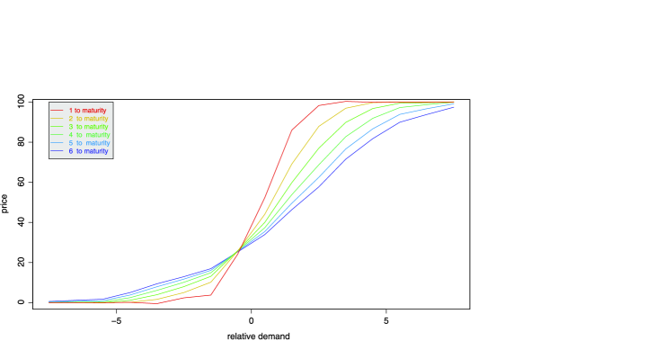
Figure 1: The functions $\alpha_{t}$ for $t=T-1,\ldots,T-6$, from the least-squares Monte Carlo method.

We now formulate an algorithm for the approximate calculation of (58) in which the conditional expectation is replaced by the least-squares Monte Carlo projection. To ease notation, let us suppose that $(\varepsilon_{t})_{t=1}^{T}$ are identically distributed (in addition to their independence (54)).

1. Initialization. Given sample $S=(e_{k},g_{k})_{k=1}^{K}\subset\mathbb{R}^{2}$ describing the distribution of $Q^{\varepsilon_{1}}\otimes\mu$ and a set of basis functions $\Psi=(\psi_{i})_{j=1}^{J}$ on $\mathbb{R}$, define $M$ as in (5). Set $\alpha_{T}(g)=1_{[0,\infty[}(g)$ for all $g\in\mathbb{R}$ and proceed in the next step with $t:=T-1$.

2. Iteration. Define $\alpha^{0}_{t}=\alpha_{t}$ and proceed in the next step with $n:=0$.

   1. [(2b)]

   2. Calculate $\phi^{n+1}(S):=(\alpha_{t+1}(g_{k}-c_{t}(\alpha^{n}_{t}(g_{k}))+e_{k}))_{k=1}^{K}$.

   3. Determine a solution $q^{n+1}\in\mathbb{R}^{J}$ to $M^{\top}Mq^{n+1}=M^{\top}\phi^{n+1}(S)$.

   4. Define $\alpha^{n+1}_{t}:=\sum_{j=1}^{J}q^{n+1}_{j}\psi_{j}$.

   5. If $\max_{k=1}^{K}|\alpha^{n+1}_{t}(g_{k})-\alpha^{n}_{t}(g_{k})|\geq\varepsilon$, then put $n:=n+1$ and continue with step 2a).

      If $\max_{k=1}^{K}|\alpha^{n+1}_{t}(g_{k})-\alpha^{n}_{t}(g_{k})|<\varepsilon$, then set $t:=t-1$. If $t>1$, go to step 2, otherwise finish.

To illustrate allowance price calculation via the Monte Carlo method, we consider the following numerical example. Suppose that the penalty is set at $\pi=100$ and that the martingale increments $(\varepsilon_{t})_{t=1}^{T}$ are independent, identically Normally distributed. Note that by an appropriate choice of the emission measurement scale, the standard deviation can always be normalized, thus we have assumed that each $\varepsilon_{t}$ is ${\cal N}(0.5,1)$-distributed. Further, consider the basis consisting of piecewise linear hut functions

$$\psi_{j}\mathchoice{\nobreak\,\colon}{\nobreak\,\colon}{\nobreak\,\colon\;}{\nobreak\,\colon\;}\mathbb{R}\to[0,1],\qquad x\mapsto(1-|z_{j}-x|/h)^{+}\qquad\mbox{for }x\in\mathbb{R},\ j=1,\ldots,J,$$

where the peaks $z_{1}=-(J-1)*h/2,\ldots,z_{J}=(J-1)*h/2$ are chosen to be equidistant with the distance $h>0$. For numerical illustration, we set $J=16$ and $h:=1$. Further, the sample $S=(e_{k},g_{k})_{k=1}^{K}$ for the Monte Carlo method is generated with $K=1000$ outcomes. For $(e_{k})_{k=1}^{K}$, we followed a natural choice, taking realizations of $K$ independent ${\cal N}(0.5,1)$-distributed random variables. However, since the distribution of $G_{t}$ is not known in advance, an appropriate candidate for $\mu$ seems to be the uniform distribution concentrated on the interval which is relevant for calculations. That is, the outcomes $(g_{k})_{k=1}^{K}$ are constructed by equidistant sampling of $[z_{1},z_{J}]$, ranging from $g_{1}=z_{1}=-7.5$ to $g_{K}=z_{J}=7.5$. For the cumulative volume function $c\mathchoice{\nobreak\,\colon}{\nobreak\,\colon}{\nobreak\,\colon\;}{\nobreak\,\colon\;}\mathbb{R}\to\mathbb{R},a\mapsto 0.1\sqrt{(a)^{+}}$, we observed a fast and stable convergence which gave a reasonable outcome within a few iterations. The resulting functions $(\alpha_{t})_{t=T-1}^{T-6}$ are depicted in Figure 1.

Let us outline a valuation procedure for a European call on emission allowance price.

1. Given basis functions $\Psi=(\psi_{j})_{j=1}^{J}$ and a sample $S=(e_{k},g_{k})_{k=1}^{K}\subset\mathbb{R}^{2}$ which approximates $Q^{\varepsilon_{1}}\otimes\mu$, determine $(\alpha_{t})_{t=T}^{0}$ in terms of basis coefficients using the above least-squares Monte Carlo algorithm.

2. Given maturity time $\tau\in\{1,\ldots,T\}$ of the European call, determine its pay-off $f^{\tau}_{\tau}:=(\alpha_{\tau}-K)^{+}$. Calculate least-squares projections, recursively processing for $u=\tau,\ldots,t$ as follows:

   1. [(b)]

   2. put $\phi(S)=(f^{\tau}_{u}(g_{k}-c_{u}(\alpha_{u}(g_{k}))+e_{k}))_{k=1}^{K}$;

   3. obtain $q$ as solution to $M^{\top}Mq=M\phi$;

   4. set $f^{\tau}_{u-1}=\sum_{j=1}^{J}q_{j}\psi_{j}$;

   5. if $u-1=t$, then finish, otherwise set $u:=u-1$ and return to (a).

3. Given recent allowance price $a$, calculate the state variable $g$ as solution to $a=\alpha_{t}(g)$.

4. Plug in the state variable $g$ and into function $f^{\tau}(t,\cdot)$ to obtain the price of the European call as as $f^{\tau}(t,g)$.

Let us conclude this section by sketching core ideas on continuous-time modeling. Our analysis shows that the risk-neutral allowance price evolution $(A_{t})_{t=0}^{T}$ must be described by a martingale whose terminal value is digital and depends on the intermediate values (see (19)). Suppose that the compliance period is given by an interval $[0,T]$, such that all relevant random evolutions are described by adapted stochastic processes on

$$\mbox{filtered probability space }(\Omega,{\cal F},P,({\cal F}_{t})_{t\in[0,T]})$$

(63)

$$\mbox{equipped with probability measure }Q\sim P,$$

where $Q$ represents the spot martingale measure. Given a random variable ${\cal E}_{T}$ and appropriate non-decreasing and continuous abatement functions $c_{t}:\mathbb{R}_{+}\times\Omega\to\mathbb{R}_{+}$ indexed by $t\in[0,T]$, we follow an analogy to discrete time and consider solutions $(A_{t})_{t\in[0,T]}$ to

$$A_{t}=\pi E^{Q}\bigl{(}1_{\{{\cal E}_{T}-\int_{0}^{T}c_{t}(A_{s})\,\mathrm{d}s\geq 0\}}|{\cal F}_{t}\bigr{)},\qquad t\in[0,T].$$ (64)

Our results from the discrete-time setting suggest that if

$$\cases{\mbox{the increments of the martingale }({\cal E}_{t}=E^{Q}({\cal E}_{T}|{\cal F}_{t}))_{t\in[0,T]}\mbox{ are}\cr\mbox{independent and the abatement functions }c_{t}\mathchoice{\nobreak\,\colon}{\nobreak\,\colon}{\nobreak\,\colon\;}{\nobreak\,\colon\;}\mathbb{R}_{+}\times\to\mathbb{R}_{+}\cr\mbox{are deterministic and time constant }(c_{t}=c)_{t\in[0,T]},}$$ (65)

then a solution to (64) should be expected in the functional form

$$A_{t}=\alpha(t,G_{t}),\qquad t\in[0,T],$$

with an appropriate deterministic function

$$\alpha\mathchoice{\nobreak\,\colon}{\nobreak\,\colon}{\nobreak\,\colon\;}{\nobreak\,\colon\;}[0,T]\times\mathbb{R}\mapsto\mathbb{R},\qquad(t,g)\mapsto\alpha(t,g),$$ (66)

and a state process $(G_{t})_{t\in[0,T]}$ given by

$$G_{t}={\cal E}_{t}-\int_{0}^{t}c_{s}(A_{s})\,\mathrm{d}s,\qquad t\in[0,T].$$

To illustrate how such an approach allows one to guess a solution, assume that

$$(\Omega,{\cal F},P,({\cal F}_{t})_{t\in[0,T]})\mbox{ supports the process }(W_{t},{\cal F}_{t})_{t\in[0,T]}$$

(67)

$$\mbox{of Brownian motion with respect to }Q\sim P.$$

Furthermore, we respond to (65), supposing that

$$\mathrm{d}{\cal E}_{t}=\sigma_{t}\,\mathrm{d}W_{t}\mbox{with pre-specified deterministic }(\sigma_{t})_{t\in[0,T]}\mbox{ and}$$

$$\mbox{continuous and non-decreasing abatement functions }(c_{t}=c)_{t\in[0,T]}.$$

To ensure the martingale property of $(A_{t}=\alpha(t,G_{t}))_{t\in[0,T]}$, apply the Itô formula

$$\mathrm{d}A_{t} = \mathrm{d}\alpha(t,G_{t})=\partial_{(1,0)}\alpha(t,G_{t})\,\mathrm{d}t+\partial_{(0,1)}\alpha(t,G_{t})\,\mathrm{d}G_{t}+{\textstyle\frac{1}{2}}\partial_{(0,2)}\alpha(t,G_{t})\,\mathrm{d}[G]_{t}$$

$$= \partial_{(1,0)}\alpha(t,G_{t})\,\mathrm{d}t-\partial_{(0,1)}\alpha(t,G_{t})c(\alpha(t,G_{t}))\,\mathrm{d}t+{\textstyle\frac{1}{2}}\partial_{(0,2)}\alpha(t,G_{t})\sigma^{2}_{t}\,\mathrm{d}t$$

$${}+\partial_{(0,1)}\alpha(t,G_{t})\sigma_{t}\,\mathrm{d}W_{t}$$

and claim the function $\alpha$ as a solution on $[0,T[\times\mathbb{R}$ to

$$\partial_{(1,0)}\alpha(t,g)-\partial_{(0,1)}\alpha(t,g)c(\alpha(t,g))+{\textstyle\frac{1}{2}}\partial_{(0,2)}\alpha(t,g)\sigma^{2}_{t}=0$$ (68)

with boundary condition

$$\alpha(T,g)=\pi 1_{[0,\infty[}(g)\qquad\mbox{for all }g\in\mathbb{R},$$ (69)

justified by the digital terminal allowance price. Having obtained $\alpha$ in this way, we construct the state process as the solution to the stochastic differential equation

$$\mathrm{d}G_{t}=\mathrm{d}{\cal E}_{t}-c(\alpha(t,G_{t}))\,\mathrm{d}t,\qquad G_{0}={\cal E}_{0},$$ (70)

and then determine

$$A_{t}:=\alpha(t,G_{t}),\qquad t\in[0,T].$$ (71)

Finally, this process must be verified in order to solve (64).

6 Conclusion

This article explains the logical principles underlying risk-neutral modeling of emission certificate price evolution. We show that within a realistic situation of risk-averse market players, there is no connection between social optimality and market equilibrium, but there is a useful feedback relation characterizing risk-neutral allowance price dynamics. Expressing this result in terms of fixed point equations on the level of martingales, we address the existence of its solution and elaborate on its algorithmic tractability. Furthermore, we suggest an extension of these concepts to continuous time and show that promising results can be obtained using diffusion processes. Here, emission allowances and their options can be described in terms of standard partial differential equations. Although option pricing in this framework seems to be appealing, we believe that it is not superior to our Monte Carlo method since the latter can be used in high dimensions and, more importantly, in the presence of jumps in the martingale $({\cal E}_{t})_{t=0}^{T}$. This is particularly important to describe price shocks, which may result from possible discontinuities in the information flow.

References

[1]
Benz, E. and Trueck, S. (2008).
Modeling the price dynamics of co2 emission allowances.
Energy Economics31 4–15.
[2]
Carmona, R., Fehr, F. and Hinz, J. (2009).
Optimal stochastic control and carbon price formation.
SIAM J. Control Optim.48 2168–2190.
MR2520324
[3]
Carmona, R., Fehr, F., Hinz, J. and Porchet, A. (2010).
Market designs for emissions trading schemes.
SIAM Review. To appear.
[4]
Carmona, R. and Hinz, J. (2009).
Risk neutral modeling of emission allowance prices and option
valuation.
Technical report, Princeton Univ.
[5]
Cetin, U. and Verschuere, M. (2009).
Pricing and hedging in carbon emissions markets.
Int. J. Theor. Appl. Finance12 949–967.
[6]
Chesney, M. and Taschini, L. (2008).
The endogenous price dynamics of the emission allowances: An
application to co2 option pricing.
Technical report.
[7]
Cronshaw, M. and Kruse, J.B. (1996).
Regulated firms in pollution permit markets with banking.
Journal of Regulatory Economics9 179–189.
[8]
Dales, J.H. (1968).
Pollution, Property and Prices. Toronto:
Univ. Toronto Press.
[9]
Daskalakis, G., Psychoyios, D. and Markellos, R.N. (2009).
Modeling co2 emission allowance prices and derivatives: Evidence from
the European Trading Scheme. Journal of Banking and Finance33
1230–1241.
[10]
Kabanov, Y.M. and Stricker, C. (2001).
A teachers’ note on no-arbitrage criteria.
Lecture Notes Math.1775 149–152.
MR1837282
[11]
Leiby, P. and Rubin, J. (2001).
Intertemporal permit trading for the control of greenhouse gas
emissions.
Environmental and Resource Economics19 229–256.
[12]
Longstaff, F. and Schwartz, E. (2001).
Valuing american options by simulation: A simple least-squares
approach.
Review of Financial Studies14 113–147.
[13]
Maeda, A. (2004).
Impact of banking and forward contracts on tradable permit markets.
Environmental Economics and Policy Studies6 81–102.
[14]
Montgomer, W.D. (1972).
Markets in licenses and efficient pollution control programs.
Journal of Econom. Theory5 395–418.
MR0443849
[15]
Paolella, M.S. and Taschini, L. (2008).
An econometric analysis of emissions trading allowances.
Journal of Banking and Finance32 2022–2032.
[16]
Rubin, J. (1996).
A model of intertemporal emission trading, banking and borrowing.
Journal of Environmental Economics and Management31 269–286.
[17]
Schennach, S.M. (2000).
The economics of pollution permit banking in the context of title iv
of the 1990 clean air act amendments.
Journal of Environmental Economics and Management40 189–210.
[18]
Seifert, J. Uhrig-Homburg, M. and Wagner, M. (2008).
Dynamic behavior of co2 spot prices.
Journal of Environmental Economics and Management56
180–194.
[19]
Sijm, J., Neuhoff, K. and Chen, Y. (2006).
Co2 cost pass-through and windfall profits in the power.
Climate Policy6 49–72.
[20]
Stentoft, L. (2004).
Convergence of the least squares monte carlo approach to american
option valuation.
Management Science50 576–611.
[21]
Stevens, B. and Rose, A. (2002).
A dynamic analysis of the marketable permits approach to global
warming policy: A comparison of spatial and temporal flexibility.
Journal of Environmental Economics and Management44
45–69.
[22]
Tietenberg, T. (1985).
Emissions Trading: An Exercise in Reforming Pollution Policy.
Boston: Resources for the Future.
[23]
Uhrig-Homburg, M. and Wagner, M. (2008).
Derivatives instruments in the EU emissions trading scheme, and
early market perspective.
Energy and Environment19 635–655.
[24]
Uhrig-Homburg, M. and Wagner, M. (2009).
Futures price dynamics of cO2 emissions certificates: An empirical
analysis.
Journal of Derivatives17 73–88.
[25]
Wagner, M. (2006).
co2-Emissionszertifikate, Preismodellierung und
Derivatebewertung.
Ph.D. thesis, Universität Karlsruhe.