An Efficient NR$xx$ Method for Boltzmann-BGK Equation

Abstract

In [3], we proposed a numerical regularized moment method of arbitrary order (abbreviated as NR$xx$ method) for Boltzmann-BGK equation, which makes numerical simulation using very large number of moments possible. In this paper, we are further exploring the efficiency of NR$xx$ method with techniques including the 2nd order HLL flux with linear reconstruction to improve spatial accuracy, the RKC schemes to relieve the time step length constraint by the regularization terms, and the revised Strang splitting to calculate convective and diffusive terms only once without loss of accuracy. It is validated by the numerical results that the overall efficiency is significantly improved and the convergence order is kept well.

1 Introduction

In 1949, the moment method was introduced by Grad [5] as a technique to approximate the Boltzmann equation in a macroscopic view. With proficient mathematical skills, he derived the famous 13-moment system, but the system is problematic: the hyperbolicity can only be obtained in the neighbourhood of Maxwellian, and the structure of shock wave is non-smooth when the Mach number is large (see e.g. [13, 6]). During a long time, the moment method suffers lots of criticism, and very few progresses are made before 1990s. In the recent twenty years, a number of new ideas based on the moment method have come out, such as the Jin-Slemrod regularization of the Burnett equations [9], the COET (Consistently Ordered Extended Thermodynamics) method [12], the order of magnitude approach [15], and et al. In [17], regularization based on 1st order Chapman-Enskog expansion was considered to remedy the defects of Grad’s 13 moment equations. The regularized system obtained therein was referred as R13 equations. Soon, the R20 and R26 equations are studied [11, 7] and the aspiration to extend this method for system with more moments [16] was called as R$xx$ by the authors of [17]. In [3], we proposed a numerical regularized moment method of arbitrary order for Boltzmann-BGK equation. The method is abbreviated as “NR$xx$ method” later on for convenience following the tradition. The NR$xx$ method makes it possible to investigate large moment systems, by direct numerical approximation of the regularized moment systems without deriving the explicit forms of the moment equations. The regularization in [3] is similar to the original derivation of the R13 equations [17]. And later in [4], the idea of COET [12] is adopted to revise the regularization terms, which results in a parabolic system.

Though one can escape from deriving the complex moment system, and the developing of the simulation program is greatly simplified by the NR$xx$ method, the numerical efficiency of the method in [3] should be further explored. It has been verified that the computational time is linear in the number of moments. However, a 1st order HLL numerical flux, which is over diffusive, was used in [3] for the transportation part, such that we have to use quite fine spatial grids to reduce the numerical error to a moderate level. Noting that the regularized moment system is parabolic, the time step is quadratic in the grid size. It turns out that in the 1D case, the total computational cost is cubic in the number of spatial grids. With a quite fine spatial grid to achieve enough accuracy, the numerical simulation therein is rather time consuming.

In this paper, we focus on improving the efficiency of the NR$xx$ method in [3] with some state-of-art techniques available to us. Precisely, three numerical techniques are employed:

1. Linear spatial reconstruction. The piecewise linear spatial reconstruction is able to provide a 2nd order HLL flux and greatly reduces the numerical diffusion. Owing to the absence of analytical expressions of the moment equations, the reconstruction needs to be done carefully. A conservative reconstruction is proposed, and it is numerically verified to have achieved high resolution. Although the final scheme is still of first order, the numerical error is greatly reduced. Thus much less grids are used in the computation.

2. RKC time integration scheme. The RKC time integration scheme [21] is adopted to enlarge the time step sizes. The RKC method is a Runge-Kutta type method originally designed for diffusive PDEs to provide large stability regions, while the regularized moment equations are convective-diffusive problems, where imaginary parts appear in the eigenvalues of the right hand side of the semi-discrete system. As is well known, the RKC schemes contain a parameter called as the damping factor, which allows a small imaginary perturbation of eigenvalues and is usually selected as a small positive value. In order to make the RKC scheme compatible with the convection terms, we use a large damping factor in our scheme to ensure stability. The final time step size is equivalent to the grid size, and the number of internal time steps is equivalent to the square root of the grid number. Thus the total number of time steps is essentially reduced, and no instability phenomenon apprears in our numerical test.

3. Revised Strang splitting method. With enlarged time step, the numerical accuracy can be harmed by convection-collision splitting. Therefore, the Strang splitting is utilized to win higher order of accuracy in the time direction. Usually, the implementation of the Strang splitting requires twice calculations of the collision term in one time step. For this problem, we combine the two steps of collision in the successive time steps, so only once calculation of the collision term is performed in a time step.

Several numerical examples are carried out to show the efficiency of our algorithm. Our prediction of the computational cost together with the order of convergence is validated by numerical experiments. We also compare the current method with the scheme without linear reconstruction to demonstrate much higher resolution for the one with linear reconstruction.

The rest of this paper is arranged as follows: in Section 2, we give a brief review of the Boltzmann-BGK equation and the NR$xx$ method. In Section 3, the linear reconstruction is added to the HLL numerical flux. In Section 4, the time step size is enlarged by the RKC method, and the accuracy is improved by the Strang splitting method. In Section 5, numerical examples are carried out to make illustrations. Some concluding remarks are given in Section 6.

2 The NR$xx$ method

2.1 The Boltzmann-BGK model

In the kinetic theory, it is generally accepted that the Boltzmann equation is able to describe the fluids accurately. Due to the complexity of the collision term, in the computational field, several simplified collision operators are adopted, among which the BGK model [1] is the simplest but useful. The Boltzmann-BGK equation reads

$$\frac{\partial f}{\partial t}+\boldsymbol{\xi}\cdot\nabla_{\boldsymbol{x}}f=\nu(f-f_{M}),\qquad\boldsymbol{x},\boldsymbol{\xi}\in\mathbb{R}^{D},$$ (2.1)

where $f$ is the distribution function, $\nu$ is the collision frequency, and $f_{M}$ is the local Maxwellian defined by

$$f_{M}(t,\boldsymbol{x},\boldsymbol{\xi})=\frac{\rho(t,\boldsymbol{x})}{[2\pi\theta(t,\boldsymbol{x})]^{D/2}}\exp\left(-\frac{|\boldsymbol{\xi}-\boldsymbol{u}(t,\boldsymbol{x})|^{2}}{2\theta(t,\boldsymbol{x})}\right).$$ (2.2)

Here $\rho$, $\boldsymbol{u}$ and $\theta$ are local macroscopic variables which represent the density, velocity and temperature respectively. They can be calculated from the distribution function $f$ by

$$\rho(t,\boldsymbol{x}) =\int_{\mathbb{R}^{D}}f(t,\boldsymbol{x},\boldsymbol{\xi})\,\mathrm{d}\boldsymbol{\xi},$$ (2.3)

$$\rho(t,\boldsymbol{x})\boldsymbol{u}(t,\boldsymbol{x}) =\int_{\mathbb{R}^{D}}\boldsymbol{\xi}f(t,\boldsymbol{x},\boldsymbol{\xi})\,\mathrm{d}\boldsymbol{\xi},$$ (2.4)

$$\rho(t,\boldsymbol{x})\boldsymbol{u}(t,\boldsymbol{x})+D\rho(t,\boldsymbol{x})\theta(t,\boldsymbol{x}) =\int_{\mathbb{R}^{D}}|\boldsymbol{\xi}|^{2}f(t,\boldsymbol{x},\boldsymbol{\xi})\,\mathrm{d}\boldsymbol{\xi}.$$ (2.5)

2.2 A first-order scheme for the NR$xx$ method

The NR$xx$ method is raised in [3, 4] as a new tool for the computation of large moment systems. It is based on an Hermite expansion of the distribution function:

$$f(t,\boldsymbol{x},\boldsymbol{\xi})=\sum_{\alpha\in\mathbb{N}^{D}}f_{\alpha}(t,\boldsymbol{x})\mathcal{H}_{\theta(t,\boldsymbol{x}),\alpha}\left(\frac{\boldsymbol{\xi}-\boldsymbol{u}(t,\boldsymbol{x})}{\sqrt{\theta(t,\boldsymbol{x})}}\right),$$ (2.6)

where $\alpha$ is a $D$-dimensional multi-index. $\mathcal{H}_{\theta,\alpha}$’s and $f_{\alpha}$’s act as the basis functions and the corresponding coefficients respectively, and $\mathcal{H}_{\theta,\alpha}$ is defined by

$$\mathcal{H}_{\theta,\alpha}(\boldsymbol{v})=(2\pi)^{-\frac{D}{2}}\theta^{-\frac{|\alpha|+D}{2}}\exp\left(-\frac{|\boldsymbol{v}|^{2}}{2}\right)\prod_{d=1}^{D}\mathit{He}_{\alpha_{d}}(v_{d}),$$ (2.7)

where $\mathit{He}_{n}(x)$’s are the orthogonal Hermite polynomials defined by

$$\mathit{He}_{n}(x)=(-1)^{n}\frac{\mathrm{d}^{n}}{\mathrm{d}x^{n}}\exp(-x^{2}/2).$$ (2.8)

This idea originates from [5] where the 13-moment equations are derived. In order to get a finite system, the NR$xx$ method [4] chooses an positive integer $M$ and approximate $f_{\alpha}$ with $|\alpha|=M+1$ by

$$f_{\alpha}=-\frac{\theta}{\nu}\sum_{j=1}^{D}\frac{\partial f_{\alpha-e_{j}}}{\partial x_{j}},\qquad|\alpha|=M+1.$$ (2.9)

Now that all $f_{\alpha}$’s with $|\alpha|=M+1$ have been related with $f_{\beta}$’s with $|\beta|=M$, we can get a closed moment system of all $f_{\gamma}$’s with $|\gamma|\leqslant M$ by putting the expansion (2.6) into the BGK equation (2.1).

The explicit expressions of such moment systems can be written in a uniform style for any choice of $M$, but those expressions are not convenient for computation, since they are not in a conservative form. In order to avoid an intricate process to obtain balance laws, the NR$xx$ method treats the distribution function (2.6) as a whole, instead of considering each moment $f_{\alpha}$ as an individual variable. For the construction of an applicable scheme, it is necessary to provide a method which is able to apply addition or subtraction on the following two distributions:

$$f_{1}(\boldsymbol{\xi})=\sum_{\alpha\in\mathbb{N}^{D}}f_{1,\alpha}\mathcal{H}_{\theta_{1},\alpha}\left(\frac{\boldsymbol{\xi}-\boldsymbol{u}_{1}}{\sqrt{\theta_{1}}}\right),\qquad f_{2}(\boldsymbol{\xi})=\sum_{\alpha\in\mathbb{N}^{D}}f_{2,\alpha}\mathcal{H}_{\theta_{2},\alpha}\left(\frac{\boldsymbol{\xi}-\boldsymbol{u}_{2}}{\sqrt{\theta_{2}}}\right).$$ (2.10)

Additionally, due to the cutoff, only $f_{1,\alpha}$’s and $f_{2,\alpha}$’s with $|\alpha|\leqslant M+1$ are known. In [3], the authors proposed a homotopic method to calculate a new representation of $f_{1}$:

$$f_{1}(\boldsymbol{\xi})=\sum_{\alpha\in\mathbb{N}^{D}}\tilde{f}_{1,\alpha}\mathcal{H}_{\theta_{2},\alpha}\left(\frac{\boldsymbol{\xi}-\boldsymbol{u}_{2}}{\sqrt{\theta_{2}}}\right),$$ (2.11)

where the coefficients $\tilde{f}_{1,\alpha}$’s with $|\alpha|\leqslant M+1$ can be worked out by solving the ODE system

$$\left\{\begin{array}[]{l}\displaystyle\frac{\mathrm{d}}{\mathrm{d}\tau}F_{\alpha}=[1-\tau R(\tau)]^{2}\sum_{d=1}^{D}\left[R(\tau)\theta_{1}F_{\alpha-2e_{d}}+(u_{1,d}-u_{2,d})\sqrt{\theta_{1}/\theta_{2}}F_{\alpha-e_{d}}\right],\\ F_{\alpha}(0)=f_{1,\alpha}\end{array}\right.$$ (2.12)

for all $|\alpha|\leqslant M+1$ until $\tau=1$, and setting $\tilde{f}_{1,\alpha}=F_{\alpha}(1)$. In Eq. (2.12), $R(\tau)$ is defined as

$$R(\tau)=\frac{\sqrt{\theta_{1}}-\sqrt{\theta_{2}}}{(\sqrt{\theta_{1}}-\sqrt{\theta_{2}})\tau-\sqrt{\theta_{2}}}.$$ (2.13)

The system (2.12) will be solved by a Runge-Kutta type scheme. Once the form (2.11) is obtained, $f_{1}+f_{2}$ or $f_{1}-f_{2}$ can be calculated naturally.

By solving (2.12), we are able to represent $f$ for any $\boldsymbol{u}^{\prime}$ and $\theta^{\prime}$ as

$$f(\boldsymbol{\xi})=\sum_{|\alpha|\leqslant M+1}f_{\alpha}^{\prime}\mathcal{H}_{\theta^{\prime},\alpha}\left(\frac{\boldsymbol{\xi}-\boldsymbol{u}^{\prime}}{\sqrt{\theta^{\prime}}}\right)+\cdots,$$ (2.14)

once there is one such representation known for some particular $\boldsymbol{u}^{\prime}$ and $\theta^{\prime}$. Here the ellipsis means the remaining coefficients are unknown. For any $\boldsymbol{u}^{\prime}$ and $\theta^{\prime}$ and the associated representation of $f$ (2.14), we have

$$\rho =\int_{\mathbb{R}^{D}}f(\boldsymbol{\xi})\,\mathrm{d}\boldsymbol{\xi}=f_{0}^{\prime},$$ (2.15)

$$\rho u_{d} =\int_{\mathbb{R}^{D}}\xi_{d}f(\boldsymbol{\xi})\,\mathrm{d}\boldsymbol{\xi}=f_{0}^{\prime}u_{d}^{\prime}+f_{e_{d}}^{\prime},\quad d=1,\cdots,D,$$

$$\rho|\boldsymbol{u}|^{2}+D\rho\theta =\int_{\mathbb{R}^{D}}|\boldsymbol{\xi}|^{2}f(\boldsymbol{\xi})\,\mathrm{d}\boldsymbol{\xi}=\rho|\boldsymbol{u}^{\prime}|^{2}+\sum_{d=1}^{D}(\theta^{\prime}f_{0}^{\prime}+2f_{e_{d}}^{\prime}u_{d}^{\prime}+2f_{2e_{d}}^{\prime}).$$

When $\boldsymbol{u}^{\prime}=\boldsymbol{u}$ and $\theta^{\prime}=\theta$, (2.14) is called as the standard representation of $f$. Note that the coefficients in (2.6) and (2.9) are in the sense of standard representation.

Another important technique is to calculate the flux $\boldsymbol{\xi}f$ based on the Hermite expansion of $f$. Since only the moments with $|\alpha|\leqslant M+1$ are known, $\boldsymbol{\xi}f$ can only be accurately given upto the $M$-th order moments. Suppose $f$ is presented as (2.14) for some $\boldsymbol{u}^{\prime}$ and $\theta^{\prime}$, and we let

$$F_{j}(\boldsymbol{\xi})=\xi_{j}f(\boldsymbol{\xi})=\sum_{|\alpha|\leqslant M}F_{j,\alpha}^{\prime}\mathcal{H}_{\theta^{\prime},\alpha}\left(\frac{\boldsymbol{\xi}-\boldsymbol{u}^{\prime}}{\sqrt{\theta^{\prime}}}\right)+\cdots,\quad j=1,\cdots,D.$$ (2.16)

Then, by making use of the recurrence relation of the Hermite polynomials, we have

$$F_{j,\alpha}^{\prime}=\theta^{\prime}f_{\alpha-e_{j}}^{\prime}+u_{j}^{\prime}f_{\alpha}^{\prime}+(\alpha_{j}+1)f_{\alpha+e_{j}}^{\prime},\quad|\alpha|\leqslant M.$$ (2.17)

Here $f_{\alpha-e_{j}}^{\prime}$ is taken to be zero if $\alpha=0$.

Once the linear operations between discrete distributions and the calculation of the flux are applicable, the convection progress can be simulated by a Riemann-solver-free finite volume method, such as Lax-Friedrichs scheme and HLL scheme (see e.g. [10]). Suppose the problem is one-dimensional, and the spatial mesh is uniform with mesh size $\Delta x$. We denote by $f_{i}^{n}$ the distribution function on the $i$-th grid at the time step $t_{n}$. Other symbols such as $\boldsymbol{u}_{i}^{n}$ and $\theta_{i}^{n}$ are defined similarly. Then, a first-order scheme with HLL numerical flux can be described as follows:

1. Let $n=0$ and set $f_{i}^{n}(\boldsymbol{\xi})$ to be the initial value, which is in its standard representation.

2. Apply (2.9) to obtain the $(M+1)$-st order moments:

   $$f_{i,\alpha}^{n}=-\frac{\theta_{i}^{n}}{\nu_{i}^{n}}\frac{f_{i+1,\alpha-e_{1}}^{n}-f_{i-1,\alpha-e_{1}}^{n}}{2\Delta x},\quad|\alpha|=M+1.$$ (2.18)

3. Solve the convection part with the HLL scheme:

   $$f_{i}^{n*}(\boldsymbol{\xi})=f_{i}^{n}(\boldsymbol{\xi})-\frac{\Delta t}{\Delta x}[G_{i+1/2}^{n}(\boldsymbol{\xi})-G_{i-1/2}^{n}(\boldsymbol{\xi})],$$ (2.19)

   where

   $$G_{i+1/2}^{n}(\boldsymbol{\xi})=\left\{\begin{array}[]{ll}\xi_{1}f_{i}^{n}(\boldsymbol{\xi}),&0\leqslant\lambda_{i+1/2}^{L},\\[5.0pt] \dfrac{\lambda_{i+1/2}^{R}\xi_{1}f_{i}^{n}(\boldsymbol{\xi})-\lambda_{i+1/2}^{L}\xi_{1}f_{i+1}^{n}(\boldsymbol{\xi})}{\lambda_{i+1/2}^{R}-\lambda_{i+1/2}^{L}}\\[15.0pt] \qquad+\dfrac{\lambda_{i+1/2}^{L}\lambda_{i+1/2}^{R}[f_{i+1}^{n}(\boldsymbol{\xi})-f_{i}^{n}(\boldsymbol{\xi})]}{\lambda_{i+1/2}^{R}-\lambda_{i+1/2}^{L}},&\lambda_{i+1/2}^{L}<0<\lambda_{i+1/2}^{R},\\[15.0pt] \xi_{1}f_{i+1}^{n}(\boldsymbol{\xi}),&0\geqslant\lambda_{i+1/2}^{R}.\end{array}\right.$$ (2.20)

   In Eq. (2.20), the signal speed $\lambda_{i+1/2}^{L}$ and $\lambda_{i+1/2}^{R}$ are approximated by

   $$\lambda_{i+1/2}^{L} =\min\left\{u_{1,i}^{n}-C_{M+1}\sqrt{\theta_{i}^{n}},\>u_{1,i+1}^{n}-C_{M+1}\sqrt{\theta_{i+1}^{n}}\right\},$$ (2.21)

   $$\lambda_{i+1/2}^{R} =\max\left\{u_{1,i}^{n}+C_{M+1}\sqrt{\theta_{i}^{n}},\>u_{1,i+1}^{n}+C_{M+1}\sqrt{\theta_{i+1}^{n}}\right\},$$

   where $C_{M+1}$ is the maximal root of Hermite polynomial $\mathit{He}_{M+1}(x)$. Eq. (2.21) is also used to determine the time step $\Delta t$. We refer to [3] for details. Note that (2.19) is only accurate up to the $M$th order moments.

4. Solve the collision part analytically:

   1. For each $f_{i}^{n*}(\boldsymbol{\xi})$, get its standard representation using (2.12) and (2.15). We suppose the result is

      $$f_{i}^{n*}(\boldsymbol{\xi})=\sum_{|\alpha|\leqslant M}f_{i,\alpha}^{n*}\mathcal{H}_{\theta_{i}^{n+1},\alpha}\left(\frac{\boldsymbol{\xi}-\boldsymbol{u}_{i}^{n+1}}{\sqrt{\theta_{i}^{n+1}}}\right)+\cdots.$$ (2.22)

   2. Multiply all coefficients $f_{i,\alpha}^{n*}$, $|\alpha|\geqslant 2$ by $\exp(-\nu\Delta t)$. The result is

      $$f_{i}^{n+1}(\boldsymbol{\xi})=\sum_{|\alpha|\leqslant M}f_{i,\alpha}^{n+1}\mathcal{H}_{\theta_{i}^{n+1},\alpha}\left(\frac{\boldsymbol{\xi}-\boldsymbol{u}_{i}^{n+1}}{\sqrt{\theta_{i}^{n+1}}}\right)+\cdots,$$ (2.23)

      where

      $$f_{i,\alpha}^{n+1}=\left\{\begin{array}[]{ll}f_{i,\alpha}^{n*},&|\alpha|<2,\\[5.0pt] f_{i,\alpha}^{n*}\exp(-\nu_{i}^{n}\Delta t),&|\alpha|\geqslant 2.\end{array}\right.$$ (2.24)

5. Increase $n$ by $1$ and return to step 2.

In step 3, since diffusion terms exist in the equations, the time step satisfies $\Delta t=O(\Delta x^{2})$. The whole scheme is of first order.

3 A high resolution scheme

As is well known, the first-order HLL flux (2.20) adds excessive diffusion to the numerical solution in a general case. In order to reduce numerical diffusion, the technique of linear reconstruction is introduced below to the finite volume method. Suppose the boundary between the $i$-th and $(i+1)$-st cells is located at $x=x_{i+1/2}$. Our aim is to construct two distributions $f_{i+1/2}^{L}(\boldsymbol{\xi})$ and $f_{i+1/2}^{R}(\boldsymbol{\xi})$ based on all cell averages $f_{i}$ to approximate the left and right limit of $f(x,\boldsymbol{\xi})$ at point $x=x_{i+1/2}$. In this section, the superscript $n$ will be omitted since the reconstruction is only applied on the same time step. Thus the numerical flux in (2.19) can be re-formulated as

$$G_{i+1/2}(\boldsymbol{\xi})=\left\{\begin{array}[]{ll}\xi_{1}f_{i+1/2}^{L}(\boldsymbol{\xi}),&0\leqslant\lambda_{i+1/2}^{L},\\[5.0pt] \dfrac{\lambda_{i+1/2}^{R}\xi_{1}f_{i+1/2}^{L}(\boldsymbol{\xi})-\lambda_{i+1/2}^{L}\xi_{1}f_{i+1/2}^{R}(\boldsymbol{\xi})}{\lambda_{i+1/2}^{R}-\lambda_{i+1/2}^{L}}\\[15.0pt] \qquad+\dfrac{\lambda_{i+1/2}^{L}\lambda_{i+1/2}^{R}[f_{i+1/2}^{R}(\boldsymbol{\xi})-f_{i+1/2}^{L}(\boldsymbol{\xi})]}{\lambda_{i+1/2}^{R}-\lambda_{i+1/2}^{L}},&\lambda_{i+1/2}^{L}<0<\lambda_{i+1/2}^{R},\\[15.0pt] \xi_{1}f_{i+1/2}^{R}(\boldsymbol{\xi}),&0\geqslant\lambda_{i+1/2}^{R},\end{array}\right.$$ (3.1)

where

$$\lambda_{i+1/2}^{L} =\min\left\{u_{1,i+1/2}^{L}-C_{M+1}\sqrt{\theta_{i+1/2}^{L}},\>u_{1,i+1/2}^{R}-C_{M+1}\sqrt{\theta_{i+1/2}^{R}}\right\},$$ (3.2)

$$\lambda_{i+1/2}^{R} =\max\left\{u_{1,i+1/2}^{L}+C_{M+1}\sqrt{\theta_{i+1/2}^{L}},\>u_{1,i+1/2}^{R}+C_{M+1}\sqrt{\theta_{i+1/2}^{R}}\right\}.$$

During the reconstruction, different methods are applied to the convection part ($|\alpha|\leqslant M$) and the diffusion part ($|\alpha|=M+1$).

3.1 Reconstruction for the convection part

For the convection part, it is important that the quantities used in reconstruction are conservative variables. Before reconstruction, according to the algorithm described in section 2.2, we already have the standard representations for all distributions $f_{i}(\boldsymbol{\xi})$, and the coefficients are assumed to be $f_{i,\alpha}$, $|\alpha|\leqslant M$. The simplest idea is to use $f_{i,\alpha}$ together with $\boldsymbol{u}_{i}$ and $\theta_{i}$ to make linear reconstruction:

$$\begin{gathered}f_{i-1/2,\alpha}^{R}=f_{i,\alpha}-g_{i,\alpha}\Delta x/2,\quad f_{i+1/2,\alpha}^{L}=f_{i,\alpha}+g_{i,\alpha}\Delta x/2,\\ \boldsymbol{u}_{i-1/2}^{R}=\boldsymbol{u}_{i}-\boldsymbol{g}_{i}\Delta x/2,\quad\boldsymbol{u}_{i+1/2}^{L}=\boldsymbol{u}_{i}+\boldsymbol{g}_{i}\Delta x/2,\\ \theta_{i-1/2}^{R}=\theta_{i}-g_{i}\Delta x/2,\quad\theta_{i+1/2}^{L}=\theta_{i}+g_{i}\Delta x/2,\end{gathered}$$ (3.3)

and

$$\begin{gathered}f_{i-1/2}^{R}(\boldsymbol{\xi})=\sum_{|\alpha|\leqslant M}f_{i-1/2,\alpha}^{R}\mathcal{H}_{\theta_{i-1/2}^{R},\alpha}\left(\frac{\boldsymbol{\xi}-\boldsymbol{u}_{i-1/2}^{R}}{\sqrt{\theta_{i-1/2}^{R}}}\right)+\cdots,\\ f_{i+1/2}^{L}(\boldsymbol{\xi})=\sum_{|\alpha|\leqslant M}f_{i+1/2,\alpha}^{L}\mathcal{H}_{\theta_{i+1/2}^{L},\alpha}\left(\frac{\boldsymbol{\xi}-\boldsymbol{u}_{i+1/2}^{L}}{\sqrt{\theta_{i+1/2}^{L}}}\right)+\cdots,\end{gathered}$$ (3.4)

where $g_{i,\alpha}$ and $g_{i}$ are constants, and $\boldsymbol{g}_{i}$ is a constant vector. However, this method leads to incorrect numerical results since none of the variables in Eq. (3.3) is conservative.

We take the original idea of the NR$xx$ method, and consider the distribution function as a whole. Thus, linear reconstruction means taking the following approximation of $f_{i-1/2}^{R}(\boldsymbol{\xi})$ and $f_{i+1/2}^{L}(\boldsymbol{\xi})$:

$$f_{i-1/2}^{R}(\boldsymbol{\xi})=f_{i}(\boldsymbol{\xi})-\frac{\Delta x}{2}g_{i}(\boldsymbol{\xi}),\quad f_{i+1/2}^{L}(\boldsymbol{\xi})=f_{i}(\boldsymbol{\xi})+\frac{\Delta x}{2}g_{i}(\boldsymbol{\xi}).$$ (3.5)

Here $g_{i}(\boldsymbol{\xi})$ is a distribution. Obviously, the most convenient representation of $g_{i}(\boldsymbol{\xi})$ is

$$g_{i}(\boldsymbol{\xi})=\sum_{|\alpha|\leqslant M}g_{i,\alpha}\mathcal{H}_{\theta_{i},\alpha}\left(\frac{\boldsymbol{\xi}-\boldsymbol{u}_{i}}{\sqrt{\theta_{i}}}\right)+\cdots.$$ (3.6)

Thus no ODEs are to be solved during the calculation of (3.5). Now, the coefficients $g_{i,\alpha}$’s can be naturally given if we represent $f_{i-1}(\boldsymbol{\xi})$ and $f_{i+1}(\boldsymbol{\xi})$ as

$$\begin{gathered}f_{i-1}(\boldsymbol{\xi})=\sum_{|\alpha|\leqslant M}f_{i-1,\alpha}^{i}\mathcal{H}_{\theta_{i},\alpha}\left(\frac{\boldsymbol{\xi}-\boldsymbol{u}_{i}}{\sqrt{\theta_{i}}}\right)+\cdots,\\ f_{i+1}(\boldsymbol{\xi})=\sum_{|\alpha|\leqslant M}f_{i+1,\alpha}^{i}\mathcal{H}_{\theta_{i},\alpha}\left(\frac{\boldsymbol{\xi}-\boldsymbol{u}_{i}}{\sqrt{\theta_{i}}}\right)+\cdots.\end{gathered}$$ (3.7)

In the implementation, we use the simplest minmod slope limiter for reconstruction

$$g_{i,\alpha}=\mathrm{minmod}\left\{\frac{f_{i+1,\alpha}^{i}-f_{i,\alpha}}{\Delta x},\frac{f_{i,\alpha}-f_{i-1,\alpha}^{i}}{\Delta x}\right\}.$$ (3.8)

This reconstruction is a conservative reconstruction, since

$$\int_{x_{i-1/2}}^{x_{i+1/2}}\tilde{f}_{i}(x,\boldsymbol{\xi})=\Delta xf_{i}(\boldsymbol{\xi}),\quad\forall i\in\mathbb{Z},$$ (3.9)

where $\tilde{f}_{i}(x,\boldsymbol{\xi})$ is a linear function of $x$ defined on $(x_{i-1/2},x_{i+1/2})$ as

$$\tilde{f}_{i}(x,\boldsymbol{\xi})=f_{i}(\boldsymbol{\xi})+g_{i}(\boldsymbol{\xi})\left(x-\frac{x_{i-1/2}+x_{i+1/2}}{2}\right),\quad x\in(x_{i-1/2},x_{i+1/2}).$$ (3.10)

However, this condition is not satisfied by the reconstruction (3.3).

3.2 Reconstruction for the diffusion part

The diffusion terms (2.9) provide approximation to the $(M+1)$-st order moments. Since (2.9) is in the sense of standard representation, we first need to get the standard representations of $f_{i-1/2}^{R}(\boldsymbol{\xi})$ and $f_{i+1/2}^{L}(\boldsymbol{\xi})$, and we use (3.4) to denote the results. The reconstruction of $f_{i-1/2,\alpha}^{R}$ and $f_{i+1/2,\alpha}^{L}$ with $|\alpha|=M+1$, which are involved in the ellipsis of Eq. (3.4), is a direct discretization of (2.9):

$$\begin{array}[]{l}f_{i-1/2,\alpha}^{R}=-\dfrac{\theta_{i-1/2}^{R}}{\nu_{i-1/2}^{R}}\dfrac{f_{i,\alpha-e_{1}}-f_{i-1,\alpha-e_{1}}}{\Delta x},\\ f_{i+1/2,\alpha}^{L}=-\dfrac{\theta_{i+1/2}^{L}}{\nu_{i+1/2}^{L}}\dfrac{f_{i+1,\alpha-e_{1}}-f_{i,\alpha-e_{1}}}{\Delta x},\end{array}\qquad|\alpha|=M+1.$$ (3.11)

Now we give a general discussion on the order of accuracy. The time splitting introduces an error of magnitude $O(\Delta t)=O(\Delta x^{2})$. With (3.5), (3.6) and (3.8), the numerical flux (3.1) turns out to be a second order numerical flux. However, as discussed in [18, 20], due to the one-sided approximation of the diffusive gradients (3.11), the final accuracy only appears to be the first order. However, comparing with the original scheme described in Section 2.2, numerical error is significantly reduced by the linear reconstruction.

4 Enlarging the time step

The regularization of the moment method introduces diffusion terms into the system, which yields a relatively small time step $\Delta t=O(\Delta x^{2})$. In order to enlarge the time step length, we use the RKC time stepping in the temporal discretization. In this section, a large time-stepping scheme with 2nd-order time integration will be proposed.

4.1 The RKC time-stepping

The RKC method is a series of explicit Runge-Kutta schemes for parabolic problems with large stability region and good internal stability. Our aim is to use $\Delta t=O(\Delta x)$ in our algorithm without producing errors larger than the original method. Thus a second-order RKC scheme is needed. The $s$-stage second-order RKC formula for the ODE system

$$w^{\prime}(t)=F(w(t))$$ (4.1)

was deduced in [21] as

$$W_{0}=w^{n},$$ (4.2)

$$W_{1}=W_{0}+\tilde{\mu}_{1}\Delta tF_{0},$$

$$W_{j}=(1-\mu_{j}-\nu_{j})W_{0}+\mu_{j}W_{j-1}+\mu_{j}W_{j-2}+\tilde{\mu}_{j}\Delta tF_{j-1}+\tilde{\gamma}_{j}\Delta tF_{0},\quad j=2,\cdots,s,$$

$$w^{n+1}=W_{s},$$

where $F_{k}=F(W_{k})$, $\tilde{\mu}_{1}=b_{1}\omega_{1}$, and

$$\mu_{j}=\frac{2b_{j}\omega_{0}}{b_{j-1}},\quad\nu_{j}=-\frac{b_{j}}{b_{j-2}},\quad\tilde{\mu}_{j}=\frac{2b_{j}\omega_{1}}{b_{j-1}},\quad\tilde{\gamma}_{j}=-a_{j-1}\tilde{\mu}_{j},\qquad j=2,\cdots,s.$$ (4.3)

Here the parameters $a_{j}$, $b_{j}$, $\omega_{0}$, $\omega_{1}$ are relevant to a manually selected damping factor $\epsilon$. They are given by

$$\omega_{0}=1+\epsilon s^{2},\quad\omega_{1}=T_{s}^{\prime}(\omega_{0})/T_{s}^{\prime\prime}(\omega_{0}),$$ (4.4)

$$b_{0}=b_{1}=b_{2},\quad b_{j}=T_{j}^{\prime\prime}(\omega_{0})/(T_{j}^{\prime}(\omega_{0}))^{2},\qquad j=2,\cdots,s,$$

$$a_{j}=1-b_{j}T_{j}(\omega_{0}),\qquad j=1,\cdots,s-1,$$

where $T_{j}(x)$ is the first kind Chebyshev polynomials

$$T_{j}(x)=\cos(j\arccos x)=\cosh(j\mathop{\mathrm{arccosh}}x),\qquad j=0,1,2,\cdots.$$ (4.5)

which can also be defined by the recurrence relation

$$T_{0}(x)=1,\quad T_{1}(x)=x,\quad T_{j+1}(x)=2xT_{j}(x)-T_{j-1}(x),\qquad j=1,2,\cdots.$$ (4.6)

The damping factor $\epsilon$ is often chosen as a small positive value such that a small imaginary perturbation of the eigenvalues of $F^{\prime}(w)$ is allowable. In [8], the authors suggest that $\epsilon$ be chosen as $2/13$, which results in a reduction in the stability boundary of about 2%.

For advection-diffusion problems, the imaginary part of the eigenvalues of $F^{\prime}(w)$ may be large. Some analysis of the eigenvalue structure of upwind finite volume methods can be found in [19], where the authors show that the imaginary parts of the eigenvalues are less than $2.0$ for the second-order scheme if the time step satisfies the CFL condition of a pure advection problem. In order to ensure the stability, we follow [22] and use a large damping factor $\epsilon=10$. Thus the stability boundary is approximately given by

$$\beta(s)\approx 0.34(s^{2}-1).$$ (4.7)

In our implementation, the RKC method is only applied to the finite volume scheme (2.19). The time step is determined by

$$\frac{\lambda_{\max}\Delta t}{\Delta x}\leqslant\mathit{CFL},$$ (4.8)

where $\lambda_{\max}$ is defined as

$$\lambda_{\max}=\max_{i}\left\{\lambda_{i+1/2}^{L},\lambda_{i+1/2}^{R}\right\}.$$ (4.9)

Then, we find the smallest positive integer $s$ satisfying

$$\Delta t\left(\frac{\lambda_{\max}}{\Delta x}+\frac{2(M+1)}{(\Delta x)^{2}}\left(\frac{\theta}{\nu}\right)_{\max}\right)\leqslant\frac{1}{2}\mathit{CFL}\cdot\beta(s),$$ (4.10)

and use the $s$-stage RKC method instead of the forward Euler scheme in (2.19). The inequalities (4.8) and (4.10) give $\Delta t=O(\Delta x)$ and $s=O\left(1/\sqrt{\Delta x}\right)$, which leads to the following estimation of the total computational time:

$$t_{\mathrm{com}}\approx\frac{T}{\Delta t/s}\cdot\frac{L}{\Delta x}=O(\Delta x^{-2.5}),$$ (4.11)

where $L$ is the length of the computational domain, and $T$ is the finishing time of the computation.

4.2 The Strang splitting

When the RKC time stepping is used, according to (4.8), the time step has the same magnitude as the grid size. Thus, when the gas is dense, we can still have only the first-order accuracy due to the convection-collision splitting, which introduces an error $O(\Delta t)=O(\Delta x)$. In order to restore the time integration to a second-order one, the Strang splitting technique [14] is employed. In our algorithm, a direct usage of the Strang splitting can be described as follows:

1. Let $n=0$.

2. Determine the time step $\Delta t_{n}$.

3. Solve the collision part over a half time step of length $\Delta t_{n}/2$.

4. Solve the convection part using the second-order RKC scheme over a time step of length $\Delta t_{n}$.

5. Solve the collision part again over a half time step of length $\Delta t_{n}/2$.

6. Increase $n$ by $1$ and return to Step 2.

This scheme requires twice calculation of the collision operator in one time step, but decrease the time integration error to $O(\Delta t^{2})$. Here we introduce a method equivalent to the above Strang splitting scheme, but only once calculation of collision term is needed per time step.

According to (4.8) and (2.21), the time step determined in Step 2 is only relevant to $\boldsymbol{u}$ and $\theta$. Since the collision steps (Step 3 and Step 5) do not change these two quantities, we can actually calculate $\Delta t_{n+1}$ before Step 5. Thus the above algorithm can be rearranged as follows:

1. Let $n=0$ and determine the time step $\Delta t_{0}$.

2. Solve the collision part over a half time step of length $\Delta t_{n}/2$.

3. Solve the convection part using the second-order RKC scheme over a time step of length $\Delta t_{n}$.

4. Determine the next time step $\Delta t_{n+1}$.

5. Solve the collision part over a half time step of length $\Delta t_{n}/2$, and then solve the collision part again over a half time step of length $\Delta t_{n+1}/2$.

6. Increase $n$ by $1$ and return to Step 3.

Recall that for the BGK model, the collision part can be solved analytically as (2.23) and (2.24). Therefore, we can replace Step 5 by

1. Solve the collision part over a time step of length $(\Delta t_{n}+\Delta t_{n+1})/2$.

Thus, the numerical result is identical to the original Strang splitting scheme, but only one collision step is performed in a complete time step.

5 Numerical examples

In this section, two numerical examples are presented to validate the efficiency and accuracy of our algorithm. In all the tests, the collision frequency $\nu$ is given by a simple form $\rho/\mathit{Kn}$, which is corresponding to the Maxwell molecules. Here $\mathit{Kn}$ is the global Knudsen number, and it is slightly different from the Knudsen number defined in [2] (denoted by $\mathit{Kn}^{\prime}$) by

$$\mathit{Kn}^{\prime}=\frac{8}{5}\sqrt{\frac{2}{\pi}}Kn.$$ (5.1)

The CFL number is chosen to be $0.95$. All the computations are performed on the Dell OptiPlex 755 desktop computer with a dual-core processor and CPU speed 2.33GHz.

5.1 An example with smooth solution

The first example is a repetition of the 1D periodic problem in [18, 3]. The computational domain is $[-1,1]$ and the boundary condition is assumed to be periodic. The initial condition is

$$\rho_{0}(x)=2+\frac{1}{2}\cos(\pi x),\quad\boldsymbol{u}_{0}(x)=\left(1+\frac{1}{2}\sin(\pi x),\frac{1}{2}\sin(\pi x),0\right)^{T},\quad p_{0}(x)=1,$$ (5.2)

and the distribution is the local Maxwellian everywhere. The computation is stopped at $t=0.4$. We set $\mathit{Kn}=0.5$ and $M=3,6,9$. The numerical results for the density $\rho$ and temperature $\theta$ are plotted in Figure 1. Since the Knudsen number is large, the profiles of density and temperature differ a lot for different moment systems.

In order to examine the efficiency of our algorithm, we discretize the problem on a series of spatial grids with grid numbers ranging from $10$ to $200$. Using $N=2/\Delta x$, the analysis at the end of Section 4.1 gives

$$t_{\mathrm{com}}=O(N^{2.5}),\quad\Delta t=O(1/N),\quad\Delta t/s=O(1/N^{1.5}).$$ (5.3)

These results are validated by Figure 2. We can see that the large time step sizes are achieved, and the results are still stable. This leads to a remarkable reduction of the computational time.

Also, the first-order convergence rate is illustrated in Figure 3, where the “exact” solution is obtained on a mesh with $800$ grids and the $L^{1}$ errors are shown. We would like to remark that although the scheme is still of first order, the magnitude of error is much smaller than the original method. In [3], where the HLL scheme without reconstruction was utilized, the authors used $1000$ grids to obtain numerical results with similar resolution as those in Figure 1. Note that small grid size implies smaller time steps, which leads to a huge computational cost.

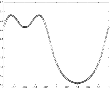
(a) $M=3$, density

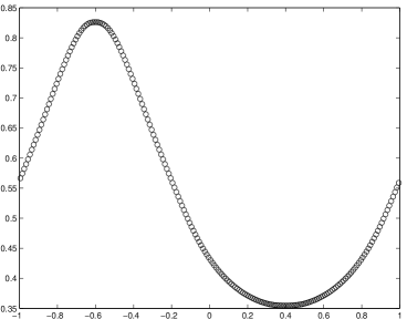
(b) $M=3$, temperature

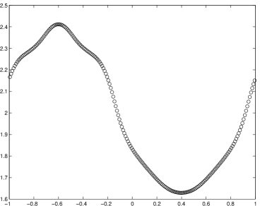
(c) $M=6$, density

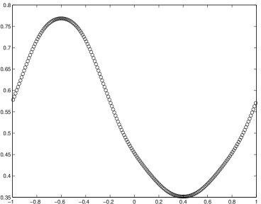
(d) $M=6$, temperature

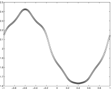
(e) $M=9$, density

(f) $M=9$, temperature

Figure 1: Numerical solutions of Problem 5.1 using $200$ spatial grids

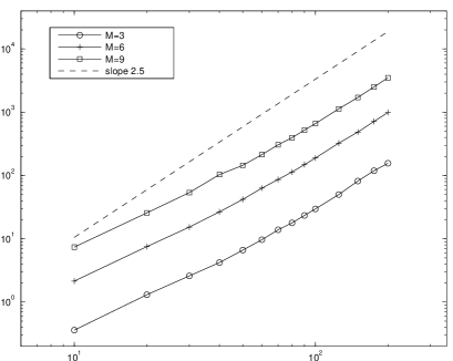
(a) Time cost $t_{\mathrm{com}}$

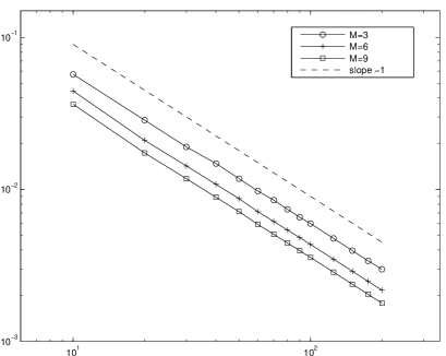
(b) Average step size $\Delta t$

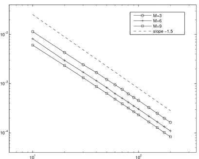
(c) Average effective step size $\Delta t/s$

Figure 2: Computational costs and time step sizes for Problem 5.1 on different spatial grids. The $x$-axis is the logarithm of the grid number $N$.

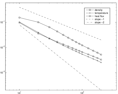
(a) $M=3$

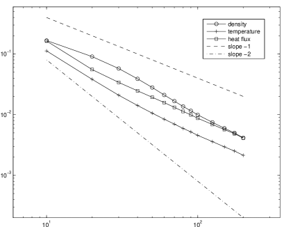
(b) $M=6$

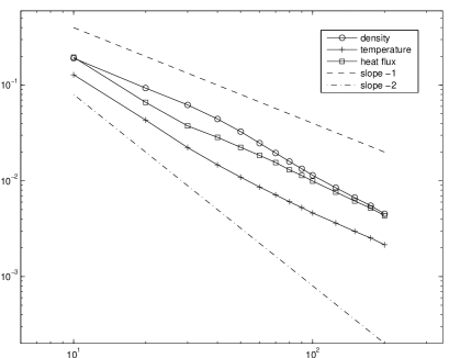
(c) $M=9$

Figure 3: Convergence rates for different moment systems

5.2 The shock-tube test

In this example, we show that our method is able to achieve high resolution when sharp layers exist in the numerical solution. Here a Riemann shock-tube problem is considered. It has been studied by Yang and Huang in [23] using the discrete ordinate method. The initial states are

$$(\rho,\boldsymbol{u},\theta)=\left\{\begin{array}[]{ll}(\rho_{l},\boldsymbol{u}_{l},\theta_{l}),&x<0.5,\\ (\rho_{r},\boldsymbol{u}_{r},\theta_{r}),&x>0.5\end{array}\right.$$ (5.4)

with

$$\begin{gathered}\rho_{l}=0.445,\quad\boldsymbol{u}_{l}=(0.698\sqrt{2},0,0)^{T},\quad\theta_{l}=13.21,\\ \rho_{r}=0.5,\quad\boldsymbol{u}_{r}=(0,0,0)^{T},\quad\theta_{r}=1.9.\end{gathered}$$ (5.5)

The Knudsen number are selected by setting $\mathit{Kn}^{\prime}=0.001$ in (5.1). The computational domain is set to be $[0,1]$, and we solve the problem until $t=0.1314/\sqrt{2}\approx 0.09291$ in order to match the results in [23].

Since $\mathit{Kn}$ is small, only the case $M=3$ is considered here. If large $M$ is used, the results are nearly identical to the current case. Some results are listed in the left column of Figure 4, whose validity can be confirmed by comparing them with those in [23]. In order to see the effects of reconstruction, we set $g_{i,\alpha}\equiv 0$ in (3.8) and rerun the program. The results are in the right column of Figure 4. It is obvious that the left column provides much higher resolution near the shock wave, while the right column is even unable to achieve the correct peak value for $N=100$ and $N=200$.

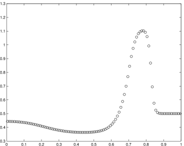
(a) $N=100$

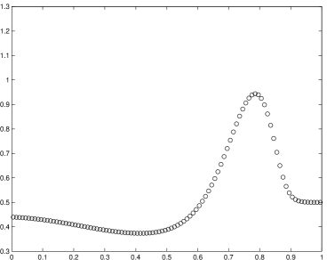
(b) $N=100$ without reconstruction

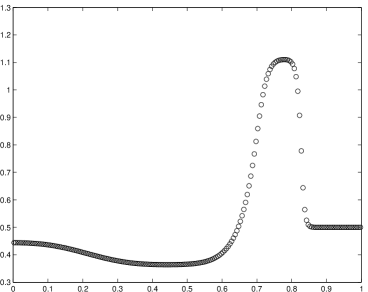
(c) $N=200$

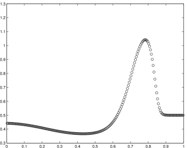
(d) $N=200$, without reconstruction

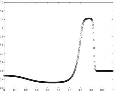
(e) $N=400$

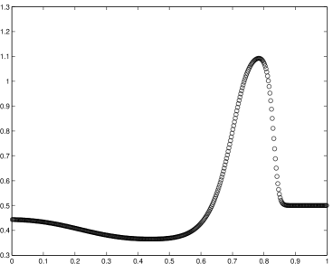
(f) $N=400$, without reconstruction

Figure 4: Density plots of the numerical solutions of Problem 5.2. $N$ is the grid number.

6 Concluding remarks

An efficient numerical scheme with high resolution for the NR$xx$ method has been presented. Since the NR$xx$ method gives a convective-diffusive system, we not only perform the linear reconstruction to gain a high spatial resolution, but also use the RKC schemes and the Strang splitting method to enlarge the time step while maintaining the order of accuracy in $\Delta x$. In the future work, we are extending it into the 2D case with unstructured grids, together with the specularly reflective boundary conditions.

References

- [1] P. L. Bhatnagar, E. P. Gross, and M. Krook. A model for collision processes in gases. I. small amplitude processes in charged and neutral one-component systems. Phys. Rev., 94(3):511–525, 1954.
- [2] G. A. Bird. Molecular Gas Dynamics and the Direct Simulation of Gas Flows. Oxford: Clarendon Press, 1994.
- [3] Z. Cai and R. Li. Numerical regularized moment method of arbitrary order for Boltzmann-BGK equation. SIAM J. Sci. Comput., 32(5):2875–2907, 2010.
- [4] Z. Cai, R. Li, and Y. Wang. Numerical regularized moment method for high Mach number flow. arXiv:1101.5787, 2010.
- [5] H. Grad. On the kinetic theory of rarefied gases. Comm. Pure Appl. Math., 2(4):331–407, 1949.
- [6] H. Grad. The profile of a steady plane shock wave. Comm. Pure Appl. Math., 5(3):257–300, 1952.
- [7] X. J. Gu and D. R. Emerson. A high-order moment approach for capturing non-equilibrium phenomena in the transition regime. J. Fluid Mech., 636:177–216, 2009.
- [8] W. Hundsdorfer and J. Verwer. Numerical Solution of Time-Dependent Advection-Diffusion-Reaction Equations. Springer, 2003.
- [9] S. Jin and M. Slemrod. Regularization of the Burnett equations via relaxation. J. Stat. Phys, 103(5–6):1009–1033, 2001.
- [10] R. J. Leveque. Finite Volume Methods for Hyperbolic Problems. Cambridge, 2002.
- [11] S. Mizzi, X. J. Gu, D. R. Emerson, R. W. Barber, and J. M. Reese. Computational framework for the regularized 20-moment equations for non-equilibrium gas flows. Int. J. Num. Meth. Fluids, 56(8):1433–1439, 2008.
- [12] I. Müller, D. Reitebuch, and W. Weiss. Extended thermodynamics – consistent in order of magnitude. Continuum Mech. Thermodyn., 15(2):113–146, 2002.
- [13] I. Müller and T. Ruggeri. Rational Extended Thermodynamics, Second Edition, volume 37 of Springer tracts in natural philosophy. Springer-Verlag, New York, 1998.
- [14] G. Strang. On the construction and comparison of difference schemes. SIAM J. Numer. Anal., 5(3):506–517, 1968.
- [15] H. Struchtrup. Derivation of 13 moment equations for rarefied gas flow to second order accuracy for arbitrary interaction potentials. Multiscale Model. Simul., 3(1):221–243, 2005.
- [16] H. Struchtrup. How many moments do we need, really? Presentation on Workshop on Moment Methods in Kinetic Theory, ETH Zürich, Switzerland, November 2008.
- [17] H. Struchtrup and M. Torrilhon. Regularization of Grad’s 13 moment equations: Derivation and linear analysis. Phys. Fluids, 15(9):2668–2680, 2003.
- [18] M. Torrilhon. Two dimensional bulk microflow simulations based on regularized Grad’s 13-moment equations. SIAM Multiscale Model. Simul., 5(3):695–728, 2006.
- [19] M. Torrilhon and R. Jeltsch. Essentially optimal explicit Runge-Kutta methods with application to hyperbolic-parabolic equations. Numer. Math., 106(2):303–334, 2007.
- [20] M. Torrilhon and K. Xu. Stability and consistency of kinetic upwinding for advection-diffusion equations. IMA J. Numer. Analy., 26(4):686–722, 2006.
- [21] P. J. van der Houwen and B. P. Sommeijer. On the internal stability of explicit, -stage Runge-Kutta methods for large -values. Z. Angew. Math. Mech., 60(10):479–485, 1980.
- [22] J. G. Verwer, B. P. Sommeijer, and W. Hundsdorfer. RKC time-stepping for advection-diffusion-reaction problems. J. Comput. Phys, 201(1):61–79, 2004.
- [23] J. Y. Yang and J. C. Huang. Rarefied flow computations using nonlinear model Boltzmann equations. J. Comput. Phys., 120(2):323–339, 1995.