A Bayesian approach to star–galaxy classification

Abstract

Star–galaxy classification is one of the most fundamental data-processing tasks in survey astronomy, and a critical starting point for the scientific exploitation of survey data. Star–galaxy classification for bright sources can be done with almost complete reliability, but for the numerous sources close to a survey’s detection limit each image encodes only limited morphological information about the source. In this regime, from which many of the new scientific discoveries are likely to come, it is vital to utilise all the available information about a source, both from multiple measurements and also prior knowledge about the star and galaxy populations. This also makes it clear that it is more useful and realistic to provide classification probabilities than decisive classifications. All these desiderata can be met by adopting a Bayesian approach to star–galaxy classification, and we develop a very general formalism for doing so. An immediate implication of applying Bayes’s theorem to this problem is that it is formally impossible to combine morphological measurements in different bands without using colour information as well; however we develop several approximations that disregard colour information as much as possible. The resultant scheme is applied to data from the UKIRT Infrared Deep Sky Survey (UKIDSS), and tested by comparing the results to deep Sloan Digital Sky Survey (SDSS) Stripe 82 measurements of the same sources. The Bayesian classification probabilities obtained from the UKIDSS data agree well with the deep SDSS classifications both overall (a mismatch rate of $0.022$, compared to $0.044$ for the UKIDSS pipeline classifier) and close to the UKIDSS detection limit (a mismatch rate of $0.068$ compared to $0.075$ for the UKIDSS pipeline classifier). The Bayesian formalism developed here can be applied to improve the reliability of any star–galaxy classification schemes based on the measured values of morphology statistics alone.

1 Introduction

Astronomical surveys now gather data on huge numbers of astronomical objects: the 2 Micron All Sky Survey (2MASS; Skrutskie et al. 2006), the Sloan Digital Sky Survey (SDSS; York et al. 2000) and the UKIRT Infrared Deep Sky Survey (UKIDSS; Lawrence et al. 2007) have all identified hundreds of millions of distinct sources. The scale of these projects immediately necessitates an automated approach to data analysis (although an intriguing alternative is The Galaxy Zoo project described by Lintott et al. 2008). Considerable effort has been put into developing algorithms which can decompose an image into a smooth background and a catalogue of discrete objects, the properties of which must be characterised as well. Source positions, fluxes and shapes can all be estimated reliably by using fairly simple moment-based approaches (e.g., Irwin 1985; Bertin & Arnouts 1996), but the separation of point-like stars from more extended galaxies generally requires at least some external astrophysical information be included. As such, the problem of star–galaxy classification is well suited to Bayesian methods in which the measurements of a given source are combined with prior knowledge of the astrophysical populations of which the source might be a member. A practical formalism for Bayesian star–galaxy classification is developed in this paper.

In Section 2 the existing methods of star–galaxy classification are reviewed, with particular emphasis on those which are at least partially Bayesian in nature. A general Bayesian formalism for star–galaxy classification is then developed in Section 3, and specialised to UKIDSS in Section 4. After analysing a simulated sample in Section 5, the real UKIDSS data are analysed – and the results compared to the classifications from deeper SDSS data – in Section 6. The relative merits of the Bayesian approach to star–galaxy classification are summarised in Section 7.

All photometry is given in the native system of the telescope in question. Thus SDSS $u$, $g$, $r$, $i$ and $z$ photometry is on the AB system, whereas UKIDSS $Y$, $J$, $H$ and $K$ photometry is Vega-based. The relevant AB to Vega conversions are given in Hewett et al. (2006).

2 Star–galaxy classification methods

The problem of systematically classifying astronomical images as either point-like (i.e., generally stars, but also quasars, etc.) or extended (i.e., generally galaxies, but also Galactic nebulae, etc.) goes back at least as far as Messier (1781), and has been the subject of many investigations in the time since. This problem is fundamental to astronomy, but there is no universally agreed upon method of solving it, and an almost bewildering number of different approaches have been explored. This is because of varying desiderata (e.g., algorithm speed; degree of automation; efficiency versus completeness; the desire for class probabilities versus absolute classification; etc.) and because different information (morphological and/or colour or even spectroscopic) is used. Hastie et al. (2008) give a general review of classification methods, but there is no astronomy-specific equivalent, so the various relevant approaches are summarised here.

The starting point for all methods of star–galaxy classification is that stars and galaxies appear different, the latter being more extended (at a given flux level) and also exhibiting more variety. For bright sources these differences are easily distinguished by the human eye (as demonstrated so well by the Galaxy Zoo project; Lintott et al. 2008); the challenge is to develop automatic algorithms that can perform the same task from measured image properties. For well-measured, high signal–to–noise ratio sources that are much brighter than a survey’s flux limit, star–galaxy separation can be achieved easily, and almost any sensible algorithm will achieve the desired results. The challenge is to treat faint sources correctly, extracting whatever morphological information is contained in the noisy measurements whilst also avoiding overly confident classification in situations of uncertainty.

The most basic, and probably most commonly used, classification method is to make simple heuristic cuts in the space of observable image properties (and related statistics, such as the measured second-order moments or kurtosis). Cuts in this space are either chosen empirically (e.g., Leauthaud et al. 2007; Kron 1980; Yasuda et al. 2001; Irwin et al. 2010) or fit to the data (e.g., MacGillivray et al. 1976; Heydon-Dumbleton et al. 1989). Such cut-based methods of star–galaxy separation have a number of benefits: they are clearly defined; they are easy to repeat or simulate; and they correctly classify the majority of sources. However cut-based methods also have several important limitations: the choice of cuts can be essentially arbitrary; it is difficult to include information about the populations as a whole; they classify every source with certainty, which is almost always unjustified close to the sample’s magnitude limits; and (partly due to the definite classification) it is difficult to combine the potentially conflicting classifications from different bands or observations.

The arbitrary nature of heuristic cuts can be avoided by using automated classification techniques. The use of neural networks, such as multi-layer perceptrons, to perform star–galaxy classification was pioneered by Odewahn et al. (1992) and forms a core part of the astronomical image analysis packages SExtractor (Bertin & Arnouts, 1996) and NExt (Andreon et al., 2000). The use of decision trees has also been explored, with both axis-parallel (Weir et al., 1995; Ball et al., 2006) and oblique (Suchkov et al., 2005) trees applied with varying degrees of success. All the above classification methods are objective, but they are also opaque, and it can be hard to predict their behaviour outside the parameter range in which they were trained and tested. The need for reliable training data can also be a problem, as this can require considerable human input and it is difficult to ensure that the necessary parameter range is covered.

Any method which decisively classifies all sources has a fundamental problem. While the images of the bright sources in any sample generally contain enough information to justify decisive classifications, many of the faint sources near a survey’s limit should not be classified with such great certainty. This issue has been tackled using a number of different techniques: mixture models (Miller & Browning, 2003); fuzzy $k$-means clustering (Mähönen & Frantti, 2000); semi-supervised clustering (Jarvis & Tyson, 1981); and difference-boosting networks (Philip et al., 2002). These methods are capable of providing non-decisive classifications, but they still tend towards over-fitting in the absence of constraining population models.

The critical point is that, for poorly-measured sources, there is potentially more information contained in the overall constraints on the star and galaxy populations than there is in the noisy image of the source in question. Including both types of information in a logically consistent way can be achieved by applying Bayes’s theorem to obtain posterior class probabilities. Contaminated samples of stars or galaxies could be obtained by adopting probability cuts, but ideally the probabilities themselves would be retained for all sources. Even though the source populations are not known perfectly, reasonable – if imprecise – models should give more realistic results for faint sources than any method which does not account for the source populations at all.

A fully principled Bayesian formalism for star–galaxy classification would involve using (parameterised) models for stars and galaxies to evaluate the conditional probabilities that a measured image was drawn from each of the two populations. Comparing these two model likelihoods then yields the posterior probability that a source is a star. For all its formal correctness, however, this is a very involved approach to inferring a single number. Indeed, none of the existing Bayesian implementations of star–galaxy classification (taken to include any method which uses information on the source populations as well as the target image) have gone to this extreme, and all adopt a variety of approximations to make the problem more tractable.

Probably the most fully principled Bayesian star–galaxy classification algorithms implemented to date are those of Sebok (1979) and Bazell & Peng (1998), who compared fits to the (calibrated) pixel values of the images. However the need to model, e.g., the spiral arms of brighter galaxies meant that, paradoxically, extra care had to be taken with the brightest images that should have been easiest to classify. This is an example of the somewhat counter-intuitive result (John, 1997) that attempting to use all the available data does not necessarily produce the most discriminating classifier, especially when machine learning methods are used (e.g., Bazell & Miller 2005; Ball et al. 2004).

The problem of galaxy complexity can be overcome by using a small number of parameters – and preferably just one – to characterise how discrepant an image is from those of similar stars observed in comparable conditions. Many morphology statistics have been developed (e.g., Irwin 1985; Scranton et al. 2005), and while they are generally not used in a Bayesian context, any such statistic can be used as a data surrogate. This fact was utilised very effectively by Scranton et al. (2002), who used the difference between the point-spread function (PSF) magnitude and the best fit galaxy profile model magnitude (defined as the concentration) as a measure of the extent of an image. However, rather than adopting parameterised models of the underlying star and galaxy populations, they fit a mixture model of Gaussians to the double-peaked $r$-band concentration distribution in a number of discrete magnitude ranges. Overall this combines simplicity and clarity whilst retaining sufficient information from the image and the populations to make excellent classifications. An obvious extension would have been to combine the data from all five SDSS bands (cf. Koo & Kron 1982; Lupton et al. 2001). In general this has proved problematic due to the combination of the different depths and the range of source colours that can, in particular, result in non-detections (e.g., Richards et al. 2004, Suchkov et al. 2005 and Ball et al. 2006 all discard objects that are not detected in all bands).

Multi-band measurements were used in a very different way by Wolf et al. (2001) (see also Richards et al. 2004), who classified sources using colour data. They utilised kernel density estimation (KDE) to calculate class densities in the space of observable quantities (in this case measured colours) and then applied Bayesian model selection to obtain a final classification. The disadvantage of this approach is the need for a large training set (in order to run the KDE on the stars and galaxies separately). The use of the noise-convolved, rather than the intrinsic, distributions can also result in sub-optimal inferences due to the inevitably greater overlap of the observed distributions.

Given the strengths and weaknesses of the various star–galaxy classification methods discussed above, we have investigated the utility of a Bayesian approach in which the star and galaxy populations are modelled parametrically and in which the data from multiple observations can be combined. The focus is on trying to obtain the best classifications for faint objects, with the provision that a decisive answer only be given if it is merited.

3 Probabilistic classification of astronomical sources

Suppose a noisy, seeing-smeared, and pixelated image of a source has been measured. What can be inferred about the type of object it is? Assuming there are ${N_{\mathrm{{t}}}}$ distinct populations of astronomical objects, $\mbox{\boldmath${{t}}$}=\{{t}_{1},{t}_{2},\ldots,{t}_{{N_{\mathrm{{t}}}}}\}$, under consideration, the fullest answer to this question is to use the available data, $\mbox{\boldmath${d}$}=\{d_{1},d_{2},\ldots,d_{N_{\mathrm{d}}}\}$, to calculate the conditional probabilities, ${\rm{Pr}}({t}|\mbox{\boldmath${d}$})$, for each ${t}$. Applying Bayes’s theorem yields

$${\rm{Pr}}({t}|\mbox{\boldmath${d}$})=\frac{{\rm{Pr}}({t})\,{\rm{Pr}}(\mbox{\boldmath${d}$}|{t})}{\sum_{{t^{\prime}}=1}^{N_{\mathrm{{t}}}}{\rm{Pr}}({t^{\prime}})\,{\rm{Pr}}(\mbox{\boldmath${d}$}|{t^{\prime}})},$$ (1)

where ${\rm{Pr}}({t})$ is the prior probability that the source is of type ${t}$ and ${\rm{Pr}}(\mbox{\boldmath${d}$}|{t})$ is the probability (density) of getting the observed data under the hypothesis that the source is of type ${t}$. Known as the evidence or the model likelihood, the latter is given by

$${\rm{Pr}}(\mbox{\boldmath${d}$}|{t})=\int{\rm{Pr}}(\mbox{\boldmath${\theta}$}_{t}|{t})\,{\rm{Pr}}(\mbox{\boldmath${d}$}|\mbox{\boldmath${\theta}$}_{t},{t})\,{\mathrm{d}}\theta_{1}\,{\mathrm{d}}\theta_{2}\,\ldots\,{\mathrm{d}}\theta_{N_{\mathrm{p}}},$$ (2)

where ${\rm{Pr}}(\mbox{\boldmath${\theta}$}_{t}|{t})$ is the usual unit-normalised prior distribution of the $N_{\mathrm{p}}$ model parameters, $\mbox{\boldmath${\theta}$}_{t}=\{\theta_{1},\theta_{2},\ldots,\theta_{N_{\mathrm{p}}}\}$, that describe objects of type ${t}$, and ${\rm{Pr}}(\mbox{\boldmath${d}$}|\mbox{\boldmath${\theta}$}_{t},{t})$ is the probability (density) of measuring the observed data given a particular value of this model’s parameters (i.e., the likelihood).

Whilst Eq. (1) is a standard application of Bayes’s theorem, its practical implementation is not so clear in an astronomical context. Demanding the prior distribution of each population’s parameters be normalised to unity is awkward, as is the notion of a prior probability of the nature of a source. Out of context, the question ‘What is the probability that a source is a star?’ does not have a sensible answer, leaving the priors undefined. Some constraining information is required, such as a range of fluxes or colours, as all probabilities are conditional. The question ‘What is the probability that a source with a magnitude of $i\leq 21.0$ is a star?’ does have a numerical answer, given approximately by the observed numbers of stars and galaxies down to the specified limit. This would yield a reasonable empirical value for the priors in Eq. (2), although even here the answer depends on Galactic latitude, due the variation in the stellar density. The implication is that the prior for each population would have to be defined differently for surveys with, e.g., different footprints on the sky or different depths, a far from satisfactory situation.

These ambiguities can be resolved by rewriting Eq. (1) as

$${\rm{Pr}}({t}|\mbox{\boldmath${d}$})=\frac{W_{t}(\mbox{\boldmath${d}$})}{\sum_{{t^{\prime}}=1}^{{N_{\mathrm{{t}}}}}W_{t^{\prime}}(\mbox{\boldmath${d}$})},$$ (3)

where we introduce the weighted evidence,

$$W_{t}(\mbox{\boldmath${d}$})=\int\rho_{t}(\mbox{\boldmath${\theta}$}_{t}){\rm{Pr}}(\mbox{\boldmath${d}$}|\mbox{\boldmath${\theta}$}_{t},{t})\,{\mathrm{d}}\theta_{1}\,{\mathrm{d}}\theta_{2}\,\ldots\,{\mathrm{d}}\theta_{N_{\mathrm{p}}}.$$ (4)

Here $\rho_{t}(\mbox{\boldmath${\theta}$}_{t})$ is the number density (per unit solid angle or per unit volume) of all type ${t}$ sources – not just those that might be detected in the survey under consideration – as a function of their parameters. For Eq. (3) to be valid, ${d}$ needs to include whether or not the source has been detected, as well as its observed properties.

The main benefit of using $\rho_{t}(\mbox{\boldmath${\theta}$}_{t})$, instead of the unit-normalised prior ${\rm{Pr}}(\mbox{\boldmath${\theta}$}_{t},{t})={\rm{Pr}}({t}){\rm{Pr}}(\mbox{\boldmath${\theta}$}_{t}|{t})$, is that the source density has an absolute, empirical and context-independent normalisation, given by the number of observed sources. Not being dependent on generally arbitrary parameter space boundaries, it is independent of the details of the current experiment, and needs only be calculated once. The detection probability is included in ${\rm{Pr}}(\mbox{\boldmath${d}$}|\mbox{\boldmath${\theta}$}_{t},{t})$, which is survey-dependent.

Equations (4) and (3) describe a general method for probabilistic classification of astronomical sources, by explicitly combining the information contained in the measurements of a source with existing knowledge of the populations from which it might have been drawn. When applied to the more specific problem of star–galaxy classification these equations simplify further still.

3.1 Star–galaxy classification

The probabilistic astronomical classification formalism described above can be applied effectively to star–galaxy classification by making several simplifying assumptions: that every source is either a star or a galaxy; that the useful morphological information in an image can be compressed into a single statistic; and that the source flux is sufficiently well measured that the uncertainty in the photometry can be ignored. Each of these approximations means the resultant class probabilities are taken away from the ideal value that would be obtained if all the available information were utilised, but the implicit information loss is only significant to the degree it changes the final classifications. As the bright, well-measured sources in any sample will be successfully classified by any sensible algorithm, it is only necessary to ensure that the useful information for the faint sources near the survey limit is retained. In the context of star–galaxy separation there is no benefit in trying to encode the wealth of morphological information present in, e.g., the image of a bright barred spiral galaxy – a statistic that accurately represented the degree to which a faint source is extended beyond the PSF is far more useful. The guiding principle in the approximations adopted here is whether they will significantly alter the classifications of the ambiguous faint sources.

How many different populations should be considered for a typical source detected in an astronomical survey? The vast majority of known sources are either Galactic stars (i.e., ${t}={\mathrm{s}}$) or galaxies (i.e., ${t}={\mathrm{g}}$). The next most common are quasars; but, as their name suggests, most appear as point–sources in the optical or near-infrared (NIR) bands, and so can be included with the stars in the context of morphological classification. Hence the set of models can reasonably be reduced to $\mbox{\boldmath${{t}}$}=\{{\mathrm{s}},{\mathrm{g}}\}$. Equation (3) can then be simplified to give the probability that a source is a star as

$$P_{\mathrm{s}}={\rm{Pr}}({\mathrm{s}}|\mbox{\boldmath${d}$})=\frac{W_{\mathrm{s}}(\mbox{\boldmath${d}$})}{W_{\mathrm{s}}(\mbox{\boldmath${d}$})+W_{\mathrm{g}}(\mbox{\boldmath${d}$})}.$$ (5)

Thus the full result of the calculation is just a single number, $P_{\mathrm{s}}$.

It is possible to simplify the problem of star–galaxy classification by considering only generic measurable properties of a source. Following the arguments in Section 2, it is assumed that each of the available images of a source provides only a single morphology statistic, $c$, which encodes the degree to which it is not point-like. There is great freedom in how $c$ is constructed from the images, and even what the fiducial stellar value is. The key point is conceptual: the potentially large data and parameter spaces are both greatly reduced by the use of a single morphology measure. The relevant data are simply the measured apparent magnitudes, $\{\hat{m}_{1},\hat{m}_{2},\ldots,\hat{m}_{N_{\mathrm{b}}}\}$, and measured morphology statistics, $\{\hat{c}_{1},\hat{c}_{2},\ldots,\hat{c}_{N_{\mathrm{b}}}\}$, in each of the $N_{\mathrm{b}}$ bands in which measurements have been made and in which the source has been detected. In general it is also necessary to include the fact that the source has been detected at all, as this is significantly greater for the faintest point-like objects near a survey’s detection limit than for extended sources. Hence the full data vector is $\mbox{\boldmath${d}$}=\{{\mathrm{det}},\hat{m}_{1},\hat{c}_{1},\hat{m}_{2},\hat{c}_{2},\ldots\hat{m}_{N_{\mathrm{b}}},\hat{c}_{N_{\mathrm{b}}}\}$, where ${\mathrm{det}}$ encodes whether the source is detected or not. The parameters used to describe a source’s observable intrinsic properties are its (true) apparent magnitudes, $\{m_{1},m_{2},\ldots,m_{N_{\mathrm{b}}}\}$, in each of the $N_{\mathrm{b}}$ bands, and its (true) morphology statistic, $c$. The full parameter vector is then $\mbox{\boldmath${\theta}$}=\{m_{1},m_{2},\ldots,m_{N_{\mathrm{b}}},c\}$.

Substituting the above definitions of ${d}$ and ${\theta}$ into Eq. (4), the weighted evidence can be written as

$$W_{t}(\mbox{\boldmath${d}$})=\int\rho_{t}(m_{1},m_{2},\ldots,m_{N_{\mathrm{b}}},c)$$ (6)

$$\,\mbox{}{\rm{Pr}}({\mathrm{det}},\hat{m}_{1},\hat{c}_{1},\hat{m}_{2},\hat{c}_{2},\ldots\hat{m}_{N_{\mathrm{b}}},\hat{c}_{N_{\mathrm{b}}}|m_{1},m_{2},\ldots,m_{N_{\mathrm{b}}},c,{t})$$

$$\,\mbox{}{\mathrm{d}}m_{1}\,{\mathrm{d}}m_{2}\,\ldots\,{\mathrm{d}}m_{N_{\mathrm{b}}}\,{\mathrm{d}}c.$$

Note that, due to the choice of observable model parameters, the likelihood now has the same form for both stars and galaxies, whereas in Eq. (2) it was population-dependent (as there was the possibility of using intrinsic physical parameters spectral type or Hubble type, which are only defined for stars and galaxies, respectively). The form of the population density and the prior can now be treated separately, and both can be usefully simplified further.

The likelihood should encode photometric uncertainties and the limitations of the morphological measurements, as well as correlations between measurements in different bands. It is, however, reasonable to assume that inter-band photometric noise correlations are negligible (but see Scranton et al. 2005), in which case the likelihood becomes a product over the $N_{\mathrm{b}}$ bands. It is also reasonable to assume that the photometric part of the likelihood is Gaussian in magnitude units – whilst this approximation breaks down for faint sources (e.g., Mortlock et al. 2010), all the sources here are unambiguously detected. It is, however, necessary to include the survey incompleteness, expressed here as the probability that a source is detected in at least one band (or, more specifically, in a reference band). The detection probability is assumed to drop from unity to zero over a magnitude range $\Delta m_{b}$ around the nominal detection limit of the survey, $m_{\mathrm{lim},b}$. The specific form adopted for the incompleteness is

$${\rm{Pr}}({\mathrm{det}}|m_{b})=\frac{1}{2}\mbox{erfc}\left(\frac{m_{b}-m_{\mathrm{lim},b}}{\Delta m_{b}}\right),$$ (7)

where $\mbox{erfc}(x)=2\int_{x}^{\infty}{\cal{N}}(2^{1/2}x^{\prime};0,1)\,{\mathrm{d}}x^{\prime}-1$ is the complementary error function, and ${\cal{N}}(x;\mu,\sigma)=\exp\{-1/2[(x-\mu)/\sigma]^{2}\}/[(2\pi)^{1/2}\sigma]$ is the unit-normalised Gaussian probability density with mean $\mu$ and variance $\sigma^{2}$. Although the detection limits for stars and galaxies are likely to be similar, the tail of this distribution is significantly longer for stars (as, being more centrally concentrated, there is a greater chance of faint stars meeting the detection criteria of most surveys). A somewhat subtle result of this is that the majority of the very faintest sources in a sample generated in this way are stars, even for surveys that are sufficiently deep that galaxies are intrinsically much more numerous at such faint fluxes.

Combining the above assumptions, the likelihood for stars and galaxies becomes

$${\rm{Pr}}({\mathrm{det}},\hat{m}_{1},\hat{c}_{1},\hat{m}_{2},\hat{c}_{2},\ldots\hat{m}_{N_{\mathrm{b}}},\hat{c}_{N_{\mathrm{b}}}|m_{1},m_{2},\ldots,m_{N_{\mathrm{b}}},c,{t})$$ (8)

$$\mbox{}=\prod_{b=1}^{N_{\mathrm{b}}}{\cal{N}}\left[\hat{m}_{b};m_{b},\sigma_{b}(m_{b})\right]{\rm{Pr}}(\hat{c}_{b}|c),$$

where $\sigma_{b}(m)$ is the magnitude-dependent noise in band $b$.For the fainter sources of most interest here (i.e., those within a few magnitudes of the relevant detection limit), the noise is background-dominated. The uncertainty for a source of magnitude $m_{b}$ in band $b$ is then

$$\sigma_{b}(m_{b})=\frac{1}{5}10^{2/5(m_{b}-m_{{\mathrm{lim}},b})},$$ (9)

where $m_{{\mathrm{lim}},b}$ is the limiting magnitude in band $b$, at which a source would be detected with, on average, a signal–to–noise ratio of 5.

The sampling distribution of $\hat{c}_{b}$ is not as generic as the distribution of $\hat{m}_{b}$ as $\hat{c}_{b}$ is necessarily a more complicated statistic, the definition of which is survey-dependent. A common choice (e.g., Irwin et al. 2010) for stars at least, is to define $c$ such that ${\rm{Pr}}(\hat{c}_{b}|c)={\cal{N}}(\hat{c}_{b};0,1)$ by construction, although even in such situations this relationship is not always satisfied empirically (cf. Section 4.5). Combined with the fact that almost nothing can be said about the form of ${\rm{Pr}}(\hat{c}_{b}|c)$ in abstract, it is left general for the moment.

The source density $\rho_{t}(m_{1},m_{2},\ldots,m_{N_{\mathrm{b}}},c)$ plays several distinct roles in Eq. (6), most obviously encoding the relative numbers of stars and galaxies at a given magnitude, but also implicitly including their distribution of colours. Making this distinction allows the more abstract source density to be separated into the number counts in a reference band, ${\mathrm{d}}N_{t}/{\mathrm{d}}m$, the conditional distribution of the (true) morphology statistic, ${\rm{Pr}}(c|m,{t})$, and a conditional magnitude-dependent colour distribution, ${\rm{Pr}}(m_{1}-m_{2},m_{2}-m_{3},\ldots,m_{N_{\mathrm{b}}-1}-m_{N_{\mathrm{b}}}|m)$. The likelihood could also be re-written as a function of one reference magnitude and colour terms $m_{1}-m_{2}$, $m_{2}-m_{3}$, etc., without loss of information. One important implication is that it is formally impossible to separate colour and morphological information in attempting to perform star–galaxy separation using multi-band data. The fact that the morphology statistic of a galaxy depends on its magnitude means that some colour-dependent calibration of this relationship is required and that this is different for stars and galaxies due to their different colours. From a Bayesian perspective this is very natural: all the available data (and external information) should be brought to bear in any inference problem, with any separability falling out as a matter of course. However star–galaxy classification is often an intermediate step towards a specific science goal, including potentially exploratory work such as searching for unusual objects. In such cases it is often desirable to use colour information alone (e.g., to search for compact galaxies, as in Drinkwater et al. 2003) or to use morphological information alone (e.g., to search for point–sources with unusual colours), but Eq. (6) shows that the two are inextricably linked. Indeed, Baldry et al. (2010) use morphology jointly with colour information to perform the galaxy target selection for the Galaxy And Mass Assembly (GAMA) survey. It is possible to produce heuristic statistics which depend only on colour or morphology, but a self-consistent Bayesian approach to star–galaxy classification must include both – or make significant approximations.

It is the latter approach that is followed here, by the potentially extreme step of ignoring the uncertainty in the measured photometry, and instead treating a source’s measured magnitude in each band, $\hat{m}_{b}$, and its true magnitude, $m_{b}$, as identical. This approximation is only justified because of this peculiar nature of the problem at hand. Given that the colour information is going to be ignored per se, the only role it will play in the model is to allow the morphology statistics of a source to be compared across bands. For example, the values of $P_{\mathrm{s}}$ calculated for two sources of different colours, but with the same values of $\hat{c}_{1}$ and $\hat{c}_{2}$, in two bands could be quite different if only one was bright enough to be well classified in a certain band. Provided that the typical value of $c$ for an object of type ${t}$ does not vary rapidly with its magnitude, it is a reasonable approximation to adopt the average colour relationships for each population.

Applying the above simplifying assumptions to Eq. (6), we obtain our final general, if approximate, expression for the weighted evidence,

$$W_{t}(\mbox{\boldmath${d}$})=$$ (10)

$$\,\mbox{}\left.\frac{{\mathrm{d}}N_{t}}{{\mathrm{d}}m}\right|_{m=\hat{m}}{\rm{Pr}}({\mathrm{det}}|\hat{m},{t})\int{\rm{Pr}}(c|m=\hat{m},{t})\prod_{b=1}^{N_{\mathrm{b}}}{\rm{Pr}}(\hat{c}_{b}|c)\,{\mathrm{d}}c,$$

where $\hat{m}$ is the measured magnitude in the reference band and ${\mathrm{d}}N_{t}/{\mathrm{d}}m$ are the differential number counts of type ${t}$ sources in this band. Note that the photometric data on the source in question only enters Eq. (10) in the estimate of the number counts and the estimate of the true morphology statistic in each band. The source’s measured values of the morphology statistic in each band are used, however, entering through the likelihood terms of the form ${\rm{Pr}}(\hat{c}_{b}|c_{b})$. Whilst it is impossible to fully escape the link between the measured shapes and colours of an object, this formalism emphasizes the former as much as is possible.

Despite the many simplifications that have been made to obtain Eq. (10), the presence of the survey-specific morphology statistic means that a more specific form of $W_{t}(\mbox{\boldmath${d}$})$ can only be obtained in the context of a specific survey or data-set. The variation in image quality and depth, combined with the different choices of morphology measure mean that the form of $P_{\mathrm{s}}$ that would be obtained by inserting Eq. (10) into Eq. (3) is our final generic result.

4 Star–galaxy classification in UKIDSS

The Bayesian approach to star–galaxy classification described in Section 3 is reasonably general and could be applied to generic optical or NIR observations. However the need for explicit population models means that its performance can only be examined in the context of specific combination of bands, depths and image quality, i.e., a particular survey. For the purpose of exploring our Bayesian approach to morphological classification we analyse data from the multi-band UKIDSS imaging survey (Section 4.1), utilising the overlap with the deeper SDSS Stripe 82 region (Section 4.2) to provide a verification sample.

4.1 UKIDSS

UKIDSS (Lawrence et al., 2007) is a suite of five separate NIR surveys using the Wide Field Camera (WFCAM; Casali et al. 2007) on the United Kingdom Infrared Telescope (UKIRT). A detailed technical description of the survey is given by Dye et al. (2006), although there have been several improvements in the time since (Warren et al., 2007). In particular, we analyse the UKIDSS Large Area Survey (LAS), which includes imaging in the UKIDSS $Y$, $J$, $H$ and $K$ bands (defined in Hewett et al. 2006) to average depths of $Y\simeq 20.2$, $J\simeq 19.6$ $H\simeq 18.8$ and $K\simeq 18.2$ (Dye et al., 2006; Warren et al., 2007). The UKIDSS data are obtained from the WFCAM Science Archive (WSA; Hambly et al. 2008), which supplies both images and processed catalogues of detected sources.

Aside from basic image parameters (e.g., positions, counts, etc.) these catalogues include a number of derived statistics, including an extendedness statistic in each band. The statistic, as defined in Irwin et al. (2010), is based on the fact that all the unsaturated stars in each field have the same average curve of growth (i.e., fraction of their total flux as a function of angular radius). This average can be measured empirically, and a mismatch statistic calculated for each source. In a given magnitude range the statistic is scaled so that, for stars, it has zero mean, unit variance and is approximately Gaussian distributed; this scaled mismatch statistic is referred to as ClassStat in the WSA. Extended galaxies (and blended pairs of sources) have positive ClassStat values, whereas most noise sources (e.g., cosmic rays), being more compact than the PSF, have negative ClassStat values. ClassStat encodes much of the important morphological information in even faint images, and is a superb morphology statistic. However because it is a statistic based solely on the image data (i.e., it does not include prior information about a source’s nature) it cannot encode all the information about a source (as distinct from the image of it). Moreover, there is no well-motivated method of combining the ClassStat values obtained from multiple measurements of a source. (In UKIDSS there are combined source probabilities and ClassStat values are reported, but these are heuristic in nature, and do not retain all the information present in the band-specific ClassStat values.)

4.2 SDSS Stripe 82

The SDSS (York et al., 2000) has surveyed $\sim 10^{4}{\mbox{\rm\,\,deg}}^{2}$ with single observations in the $u$, $g$, $r$, $i$ and $z$ bands (Fukugita et al., 1996), to depths of $\mbox{$u$}\simeq 22.0$, $\mbox{$g$}\simeq 22.2$, $\mbox{$r$}\simeq 22.2$, $\mbox{$i$}\simeq 21.3$ and $\mbox{$z$}\simeq 20.5$. The SDSS has also taken repeat measurements in the Stripe 82 region (covering the right ascension range $\alpha\leq 60$ and $\alpha\geq 300{\mbox{\rm\,\,deg}}$ and declinations of $|\delta|\leq 0.1$), reaching depths of $\mbox{$u$}\simeq 23.6$, $\mbox{$g$}\simeq 24.5$, $\mbox{$r$}\simeq 24.2$, $\mbox{$i$}\simeq 23.8$ and $\mbox{$z$}\simeq 22.1$.

The SDSS approach to star–galaxy classification is based on the use of model magnitudes, each detected source being fit as both a point–source (i.e., the measured point–spread function) and a galaxy (i.e., a Sérsic 1963 profile with one of two different exponents). The difference between the two different magnitudes, termed the concentration, $c$, is then used as a morphology statistic (Yasuda et al., 2001). The basic classification is done by designating sources with $c\leq 0.145$ as stars and sources with $c>0.145$ as galaxies. Whilst this scheme is very effective, it is also important to note that the classifications of up to a third of sources contradict in different bands (Yasuda et al., 2001).

The Stripe 82 data are significantly deeper than the UKIDSS LAS (in the sense that all but the reddest sources are detected with a greater signal–to–noise ratio in Stripe 82 than in the LAS, and an average UKIDSS-selected source has $\sigma_{r}\simeq 0.1\,\sigma_{Y}$). Even though the SDSS optical imaging has a significantly larger seeing ($\sim 1\,\aas@@fstack{\prime\prime}2$) than the UKIDSS NIR data ($\sim 0\,\aas@@fstack{\prime\prime}8$), the SDSS Stripe 82 data of the morphologically ambiguous sources near the LAS detection limit is able to separate point and extended sources reliably. This is illustrated by Figs. 1, 2 and 3. Fig. 1 shows SDSS $r$-band concentration plotted against UKIDSS $Y$-band ClassStat. For the faintest two magnitude bins ($Y\simeq 19$ and $Y\simeq 20$) it is impossible to identify two different populations of sources along the horizontal (ClassStat) axis, whereas this is still possible along the vertical (concentration) axis. This is confirmed by the one-dimensional histograms of both classification statistics [Figs. 2 (concentration) and 3 (ClassStat)]. For $Y\simeq 19$, in Fig. 3, the two populations of sources have almost completely merged, even though the histogram is still bi-modal and for $Y\simeq 20$ the two populations of sources cannot be distinguished at all. However the corresponding histograms for SDSS concentration clearly show two distinct populations of sources. In particular, for $Y\simeq 20$, the SDSS $r$-band class labels misclassify only $\sim 4\%$ of sources (this number is obtained by fitting a Gaussian distribution to the star population and a log-normal to the galaxy population for the SDSS concentration data). This is a very good result when compared to the UKIDSS ClassStat data which, at this faintness regime, no longer allow a separation into two populations of sources (Fig. 3).

Hence, for the purpose of star–galaxy separation, we treat the SDSS Stripe 82 data as definitive classifications against which our Bayesian LAS classifications can be tested.

Figure 1: SDSS $r$-band concentration plotted against UKIDSS $Y$-band ClassStat for different magnitude bins.

Figure 2: One-dimensional slices of SDSS concentration data for different magnitude bins.

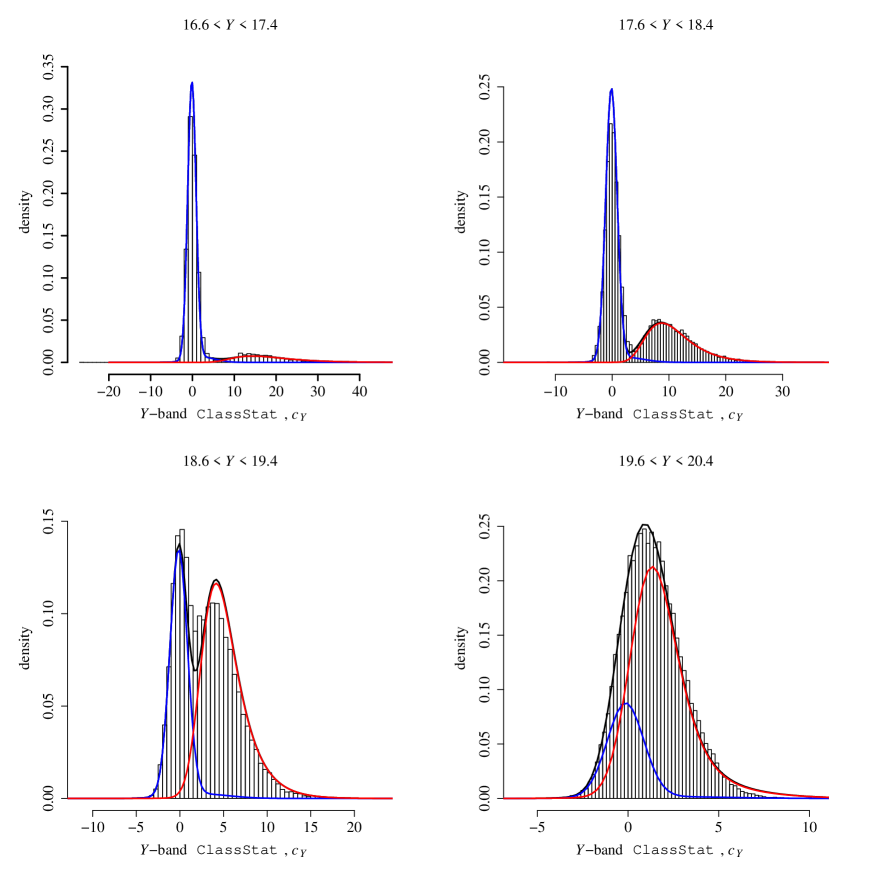
Figure 3: One-dimensional slices of UKIDSS ClassStat data for different magnitude bins. Also shown is the fit of our model [overall probability density (black line), star class probability density (blue) and galaxy class probability density (red)], which is discussed in Section 4.6 and further illustrated on Fig. 6.

4.3 Test sample

Our starting point is a sample of $121\,902$ UKIDSS sources in a $14.4{\mbox{\rm\,\,deg}}^{2}$ area defined by right ascensions of either $\alpha\leq 60{\mbox{\rm\,\,deg}}$ or $\alpha\geq 300{\mbox{\rm\,\,deg}}$ and declinations of $|\delta|\leq 0.1$. This area is entirely within the SDSS Stripe 82 region, and has been covered by UKIDSS in the $Y$, $J$, $H$ and $K$ bands. Our main aim is to classify these sources and compare the results to the SDSS Stripe 82 classifications. But to do so requires the preliminary task of generating the magnitude-dependent prior distributions of ClassStat, along with the star and galaxy number counts. This is not part of the actual classification process (i.e., it is independent of any single source), and so is considered separately from the results.

4.4 Number counts

The number counts of stars and galaxies provide the prior that will be used to classify sources for which the image data are ambiguous. The counts could be obtained from deeper surveys (although none exist in all the UKIDSS LAS bands) or from physical models of the source populations (although this would be unnecessarily complicated). For the restricted problem of star–galaxy separation, however, it is more direct to fit the star and galaxy counts to the target sample itself. At the bright end the numbers are given directly by the data; at the faint end it is also necessary to assume some weak prior information (essentially that a smooth extrapolation from the bright counts is reasonable).

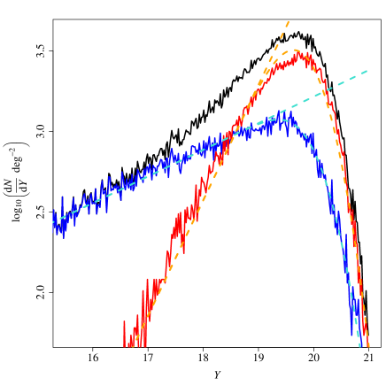
Figure 4: Differential number counts of all sources (black), stars (blue) and galaxies (red) from UKIDSS observations. Classifications are obtained by using our model with number counts obtained by binning the data into equal-sized magnitude bins and fitting simple mixture models to the $c_{Y}$ data in each bin. Also shown as dashed lines are the model fits (see Eq. (11)), both with and without a correction for incompleteness.

For the UKIDSS LAS we have chosen the $Y$ band as the reference band. The observed $Y$ band counts of stars and galaxies (identified here by using our model with number counts obtained by binning the data by magnitude and interpolating the parameters) from the test sample described in Section 4.3 are shown in Fig. 4. Both exhibit exponential counts down to $Y\simeq 19$, beyond which the survey incompleteness dominates (as expected, given the average UKIDSS LAS limit of $Y\simeq 20.2$). For both stars and galaxies the intrinsic number counts are taken to be of the form

$$\rho_{t}(Y)=\frac{{\mathrm{d}}N_{t}}{{\mathrm{d}}Y}=\alpha_{t}\ln(10)N_{t}10^{\alpha_{t}(Y-Y_{0})},$$ (11)

where $N_{t}$ is the number of sources (optionally per unit solid angle, although this detail is unimportant as long as the same normalising convention is used for stars and galaxies) of type ${t}$ brighter than the reference magnitude $Y_{0}$, and $\alpha_{t}$ is the type-dependent logarithmic slope. Even though $Y_{0}$ and $N_{t}$ are degenerate it is convenient to set $Y_{0}$ to the $Y$-band magnitude limit, in which case $N_{t}$ is approximately equal to the number of objects of type ${t}$ in the sample.

In order to fit these parameters, however, it is necessary to account for the incompleteness in each band, denoted here as ${\rm{Pr}}({\mathrm{det}}|Y)$, which was introduced in Eq. (7). The magnitude limit $m_{\mathrm{lim},b}$ and incompleteness range $\Delta m_{b}$ are fit in the $Y$, $J$, $H$ and $K$ bands for both stars and galaxies. Fitting ${{\mathrm{d}}N_{t}}/{{\mathrm{d}}Y}\,{\rm{Pr}}({\mathrm{det}}|Y)$ to the observed UKIDSS counts yields the fits shown in Fig. 4. Although there are some discrepancies, the key point is that the relative numbers of stars and galaxies at a given magnitude will give far more accurate prior probabilities than, say, an uninformative prior [i.e., ${\rm{Pr}}(s)={\rm{Pr}}(g)=0.5$ for all sources].

4.5 ClassStat distributions

ClassStat is constructed so that, on average, $c=0$ for stars and $c>0$ for extended sources. We observe $\hat{c}$ however, the distribution of which, for isolated stars should be normal (with zero mean and unit variance), again by construction. However the observed ClassStat distribution of bright stars (defined as UKIDSS sources with $13\leq Y\leq 17$ and $|c_{Y}|<6$) shown in Fig. 5 appears to be significantly non-Gaussian. This impression is confirmed by the Shapiro & Wilk (1965) and one-sample Kolmogorov–Smirnov (Conover, 1999) normality tests.

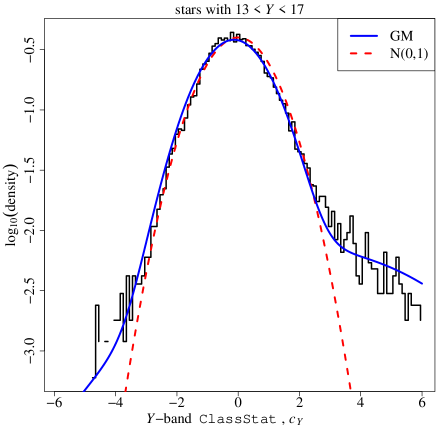
Figure 5: The empirical distribution of ClassStat values of bright ($13\leq Y\leq 17$) UKIDSS sources with $|c_{Y}|\leq 6$ (this selection region is shown on Fig. 9). Also shown is a ${\cal{N}}(0,1)$ normal distribution and the best-fit Gaussian mixture model defined in Eq. (12).

The distribution of ClassStat values for the bright stars has a slightly negative mean, and is weakly positively skewed. Due to the positive skewness, using a symmetrical distribution with larger tails than a normal (such as Student’s $t$-distribution) will not result in a good fit. For the observed ClassStat distribution we have instead adopted a Gaussian mixture model of the form

$${\rm{Pr}}(\hat{c}_{b}|c)=a{\cal{N}}(\hat{c}_{b}-c;\mu_{1},1)+(1-a){\cal{N}}(\hat{c}_{b}-c;\mu_{2},\sigma_{2}),$$ (12)

where, for stars, $c=0$, and $\mu_{1}$, $\mu_{2}$ and $\sigma_{2}$ are free parameters to be fit. These were fit using a simple maximum likelihood (ML) approach in each of the four UKIDSS bands. The resulting values are given in Table 1, and the $Y$ band fit is compared to the data in Fig. 5.

We used the Bayesian information criterion (BIC; Schwarz 1978) to assess the model fit. As expected, the Gaussian mixture model is a considerably better fit to the data than either fiducial unit-variance Gaussian, or the Gaussian with ML parameters, resulting in significantly lower BIC values.

The distribution of $c$ is more complicated for galaxies than for stars, both because galaxies are intrinsically more varied, and also because the definition of the morphology statistic is essentially independent of galaxies’ properties. For the UKIDSS sample an empirical function was sought which could represent the distribution of galaxies’ $c$ values as a function of magnitude. Particular care was taken to ensure a good fit close to the survey’s limit, for which there is minimal morphological information and $c\rightarrow 0$, even for galaxies.

These desiderata are met by a log-normal distribution:

$${\rm{Pr}}(c|\hat{m},{t}={\mathrm{g}})={\cal{L}}[c;\mu(m),\sigma(m)],$$ (13)

where

$${\cal{L}}(x;\mu,\sigma)=\frac{1}{x\sqrt{2\pi\sigma^{2}}}\exp\left\{-\frac{[\ln(x)-\mu]^{2}}{2\sigma^{2}}\right\}.$$ (14)

Rather than specifying the functions $\mu(m)$ and $\sigma(m)$ of the standard parameterisation of the log-normal distribution (Eq. 14), we have modelled the mean $\mu^{\prime}(m)$ and standard deviation $\sigma^{\prime}(m)$ of the log-normal distribution by the empirical functions below,

$$\mu^{\prime}(m)=\left(1-\frac{m}{m_{\mathrm{max}}}\right)$$ (15)

$$\qquad\qquad\qquad\times\left\{[\nu_{1}(m-\nu_{4})^{2}+\nu_{2}(m-\nu_{4})+\nu_{3}]^{\nu_{5}}+\nu_{6}\right\},$$

$$\sigma^{\prime}(m)=\eta_{1}10^{\eta_{2}(m-11)+5},$$ (16)

where $m_{\mathrm{max}}$ is the upper detection limit in the reference band and $\nu_{1},\nu_{2},\nu_{3},\nu_{4},\nu_{5},\nu_{6},\eta_{1}$ and $\eta_{2}$ are free parameters fitted by a simple least-squares (LS) procedure.

The stellar and galactic densities implied by our models are shown as contours in Fig. 6, along with the sample from which the fit was derived. (The $H$ band, rather than the $Y$ band, was chosen as it has the highest number of saturated sources, thus emphasizing an aspect of the data that is not included in the model.) The fit is not perfect (e.g., the true density is underestimated at the bright end and slightly overestimated in two regions near the faint end), but is very good. Also, the bright UKIDSS stars (with $H\la 12.5$) have significantly positive ${\tt{ClassStat}}$ values, as they are saturated; we do not attempt to include this phenomenon as essentially all sources bright enough to be saturated in UKIDSS images can be classified as stars on the basis of prior information.

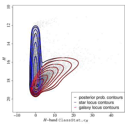
Figure 6: The distribution of UKIDSS sources (black points) and the model (contours) in the $H$ band. The case for the $H$ band is plotted as the saturation of bright sources is not as apparent in the $Y$ band. One-dimensional plots of the model fit (this time for the $Y$ band) are shown on Fig. 3.

Table 1: Maximum likelihood values, with corresponding standard errors in brackets, for the parameters of the Gaussian mixture model used for the observational noise.

band	$a$	$\mu_{1}$	$\mu_{2}$	$\sigma_{2}$
$Y$	0.9453 (0.0030)	0.1418 (0.0085)	2.3950 (0.1501)	3.2021 (0.08600)
$J$	0.9436 (0.0053)	0.1131 (0.0143)	1.1879 (0.2379)	3.7199 (0.1776)
$H$	0.9601 (0.0033)	0.1266 (0.0117)	3.3037 (0.2922)	3.7523 (0.1617)
$K$	0.9474 (0.0039)	0.0360 (0.0118)	3.6881 (0.2463)	3.4449 (0.12975)

4.6 Simulated data

Given that the distribution of magnitudes and morphology statistics described above was developed sequentially, it is important to perform an end–to–end test of the entire model.

The first stage of this was to generate a sample of simulated sources from the model. The algorithm for doing so can be broken down into several steps:

• Draw a true $Y$ band magnitude from the total (star + galaxy) number count model given in Eq. (11).

• Determine the type (star or galaxy) of the object from the relative number counts at this $Y$ band magnitude.

• Use the average $Y$$\!\,-$$J$, $Y$$\!\,-$$H$ and $Y$$\!\,-$$K$ colours for stars and galaxies (as shown in Fig. 10) to obtain $J$, $H$ and $K$ band magnitudes.

• Record the object as being detected in each band with probability given by the incompleteness formula in Eq. (7).

• Add observational (sky) noise to the true magnitudes in all bands by sampling from a Gaussian distribution with zero mean and band-dependent standard deviation given by Eq. (9).

• Generate ClassStat values for each band by sampling $c$ from Eq. (13) for galaxies, setting $c=0$ for stars and then sampling from the mixture model given in Eq. (12).

Fig. 8 shows a sample of data generated by the above procedure. Having verified that generating sources from our model can accurately mimic the relevant UKIDSS data, the model can now be used with confidence as the prior needed to perform Bayesian star–galaxy classification.

5 Analysis of simulated UKIDSS data

A first test of our Bayesian star–galaxy classification method is to analyse the simulated UKIDSS data described in Section 4.6. As the input star and galaxies distributions are known, the resultant stellar probabilities are, given the deliberately imposed restrictions on the use of colour information, optimal. In particular, the numbers and properties of the sources which cannot be classified decisively are of interest, as any real sources with such properties will have $P_{\mathrm{s}}\simeq 0.5$.

Figure 7: Histogram of the posterior star probabilities, $P_{\mathrm{s}}$, evaluated for simulated UKIDSS data.

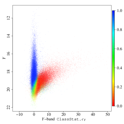
Figure 8: Combined star probabilities derived from our Bayesian method for simulated UKIDSS data.

The distribution of posterior star probabilities for all sources is shown in Fig. 7 and the distribution in $Y$ vs. $c_{Y}$ space is shown in Fig. 8. These results from simulated data can be compared to Figs. 11 (left) and 12 (left), which show the results when our method is applied to real UKIDSS data. While there is not much difference between Figs. 8 and 12 (left), there are two noticeable differences between Figs. 7 and 11 (left): there are more simulated sources with low star probabilities and there are more sources with $P_{\mathrm{s}}$ clearly different from $0$ and $1$ (i.e., not classified with certainty). In particular there are many more sources with $P_{\mathrm{s}}\la 0.4$, yet clearly non-zero. The former difference can be explained by the fact that there are fewer bright sources (which are predominantly stars and hence have high star probabilities) among the generated data. This means that for equal sample sizes there will be more sources with low star probabilities in the simulated sample when compared to the original data sample. The increase in sources with less definite classifications is due to the fact that, as acknowledged in Section 3.1, our model is not designed to take inter-band photometric noise correlations into account. Thus the simulated data sample contains more sources with seemingly contradicting ClassStat data in the different bands than a sample of real data. Both of these differences have only a small effect on the simulated data, and should affect the classification of a negligible number of real sources.

6 Results

The Bayesian method of star–galaxy classification described above was applied to the sample of UKIDSS sources in the SDSS Stripe 82 region, giving single-band star probabilities for every source detected (in each band in which the source was detected), as well as combined probabilities. The general properties of the classifier are discussed in Section 6.1, and then compared to the UKIDSS classifications (in Section 6.2) and the SDSS classifications (in Section 6.3).

6.1 Properties of the classifier

Table 2: Fraction of sources with posterior probabilities between $0.4$ and $0.6$ for both the single-band models and the joint model. The fractions for the joint model are not the same across the four bands as we only consider sources that are observed in the given bands. So while the probabilities for the joint model are obviously the same across all bands, the fractions in the table above vary across bands as the number of observed sources vary across bands.

band	$Y$	$J$	$H$	$K$
single-band model	0.0332	0.0384	0.0322	0.0336
joint model	0.0254	0.0254	0.0201	0.0155

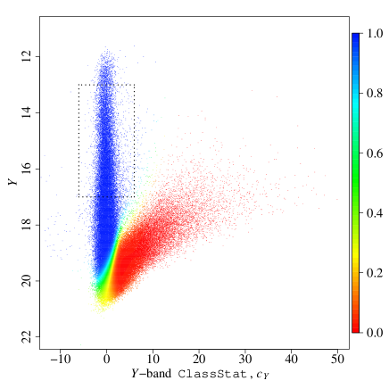
Figure 9: Single-band star class probabilities (Y band). The dotted box represents the selection region for the sources from Fig. 5.

Figure 9 shows the single-band posterior star probabilities in $Y-c_{Y}$ space. These can be compared with the probabilities obtained by using the full multi-band model (Fig. 12). The most notable difference is that for the latter case there seem to be fewer sources which confound the classifier, i.e., with $P_{\mathrm{s}}\simeq 0.5$. Table 2 lists the fraction of sources for which the classifier gives $0.4\leq P_{\mathrm{s}}\leq 0.6$. Compared to the single-band model, there is a decrease of at least $25{\mbox{\rm\,\,per cent}}$ in this number for the combined model. While a reduction in the classifier-confounding region is not always desirable, here this decrease translates the fact that the classifier will be at a loss only when the data from different bands are contradictory, or when a source’s type is unclear in all the bands in which it was detected.

Figure 10 shows the distribution of the posterior star class probabilities over $Y$$\!\,-$$H$ vs. $H$$-$$K$ space. Even though the model has not been designed to optimise class separation in colour–colour space, there are two clearly distinct populations. Furthermore, sources with low star probabilities have $\mbox{$Y$$\!\,-$$H$}\simeq 1.5$ and $\mbox{$H$$-$$K$}\simeq 0.8$, as expected.

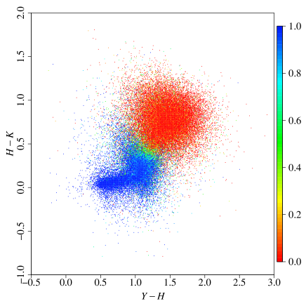
Figure 10: Colour–colour plot of the posterior star class probability vector

6.2 Comparison with UKIDSS pipeline classifications

Figure 12 (left) shows the posterior stellar probabilities in the $c_{Y}$ vs. $Y$ plane (the choice of band is unimportant, as the $J$, $H$ and $K$ band plots are similar). It is clear that for the overwhelming majority of objects, in particular those with either $Y\la 18$ or $c_{Y}\ga 5$, the Bayesian classifier gives very definite classifications (i.e., values close to either 0 or 1). Unsurprisingly, the region where the classifier is most often confounded is where the star and galaxy loci merge. Indeed, as the two loci overlap completely at the faint end, there is very little information regarding object class to be extracted from the measured ClassStat values, and the prior knowledge drives the classification.

One of the main aims of our classifier is to make the fullest possible use of whatever morphology statistic is available – the UKIDSS ClassStat statistic in the case considered here – and in particular for sources where it has been measured in multiple bands. Several heuristic methods are used to combine multiple measurements in the WSA, including simple averaging and a plausible – but again heuristic – contingency table for sources where the ClassStat measurements in different bands imply contradictory classifications. Our Bayesian method has the potential to propagate all the information contained in the individual $c$ values correctly, albeit at the cost of introducing an explicit – and complicated – model.

Figure 11: Histograms of the posterior star class probability vectors for both our model and the UKIDSS pipeline

The UKIDSS pipeline posterior star probabilities can be compared to that from our model (Fig. 12). Both classifiers yield similar posterior star probabilities for sources which are fairly bright and/or have large ClassStat values, but deal differently with faint sources with small ClassStat values. Apart from a slight shift to the left at the faint end, the UKIDSS pipeline classifier can be seen to consist essentially of a vertical cut on the ClassStat value. The classifier-confounding region (i.e., where the classifier outputs probabilities near $0.5$) is fairly small, and, crucially, does not widen at the faint end. Our classifier, however, through the input of prior knowledge, is not limited to taking a vertical cut and the classifier-confounding region is larger, particularly at the faint end. Indeed, near the detection limit, the ClassStat values carry almost no information concerning object type, as stars and galaxies have similar values at those fluxes. It thus makes very little sense to base a classification on that information. Using prior knowledge is vital for such faint sources. Our classifier allows a continuous transition from ClassStat value based classification to prior knowledge based classification. The resulting broader classifier-confounding region is not a drawback: if an object has $P_{\mathrm{s}}\simeq 0.5$, it means that, given the observed data, it is impossible to tell whether that source is a star or a galaxy. Artificially coercing posterior classifications to be unambiguous is wrong. If a source cannot be reliably classified, then its posterior probability should reflect this.

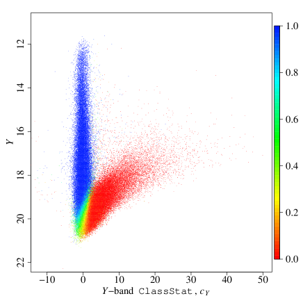
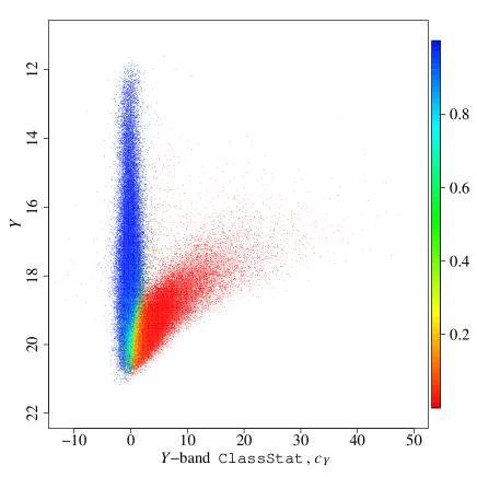
Figure 12: Combined star probabilities derived from our Bayesian method (left) and the UKIDSS pipeline (right) as a function of the measured $Y$ band ClassStat and magnitude.

Both the posterior probabilities computed by our classifier and the original, observed ClassStat values can serve as indicators of source type. While one should take a source’s flux into account when assessing its ClassStat data (cf. Fig. 12), ClassStat is designed so as to differentiate between resolved and unresolved sources, and is indeed used to this purpose by the UKIDSS pipeline. Hence it makes sense to compare the posterior class probabilities directly with the ClassStat values.

Figure 13: posterior star probabilities plotted against MergedClassStat for different magnitude bins.

Figure 13 summarises the situation for different magnitude regimes. At fairly bright magnitudes (i.e., $Y\simeq 17$) most sources have $P_{\mathrm{s}}\simeq 1$, except for obviously extended sources with very large ClassStat values. At the faint end ($Y\simeq 20$) the classifications are not so decisive with few sources having $P_{\mathrm{s}}\simeq 0$ or $P_{\mathrm{s}}\simeq 1$. The depth of the UKIDSS LAS is such that the surface density of stars and galaxies is comparable at the survey’s magnitude limit. This is the most interesting regime for star–galaxy classification problems: as significantly shallower or deeper surveys would be dominated by stars or galaxies, respectively, at their magnitude limit, and so essentially all the poorly measured sources would be decisively classified purely by the population prior.

However, very low star probabilities ($P_{\mathrm{s}}\la 0.1$) are only reached when ClassStat exceeds a certain threshold. In the region where star and galaxy populations merge (in magnitude vs. ClassStat space; $Y\simeq 19$) a trend is apparent: large ClassStat values result in low posterior star probabilities. However the reverse is not true: except for sources with extremely low ($c_{Y}<0$) or high ($c_{Y}>10$) ClassStat values, a source’s star probability does not reveal much about its ClassStat value. In the regions where stars and galaxies are fairly well separated ($Y\simeq 17$ and $Y\simeq 18$), there is a good correspondence between posterior star probability and ClassStat.

6.3 Comparison with SDSS Stripe 82 classifications

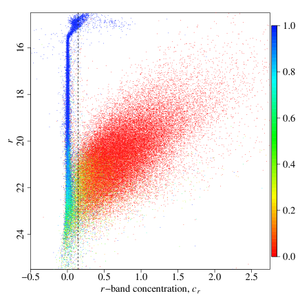
Figure 14: UKIDSS posterior star probabilities shown as a function of the measured SDSS Stripe 82 concentration vs. $r$-band magnitude. Sources to the left/right of the dotted line (with concentration = 0.145) are classified as stars/galaxies in SDSS.

Figure 14 shows the posterior star probabilities from our model as a function of SDSS concentration and $r$-band magnitude. The dotted line indicates the threshold concentration value ($0.145$) for SDSS star/galaxy labels. Overall there is good agreement with most sources with low $P_{\mathrm{s}}$ lying to the left of the line and sources with high $P_{\mathrm{s}}$ lying to the right.

For sources classified with great confidence by both classifiers [i.e., fairly bright, but non-saturated sources ($16\la r\la 21.5$) with corresponding UKIDSS posterior star probabilities above $0.9$ and SDSS concentration below $0.05$ or posterior star probabilities below $0.1$ and concentration above $0.2$], we can study those sources for which the two classifiers disagree. Figure 15 shows that most such sources lie right between the star and galaxy loci.

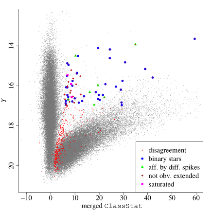
Figure 15: The full sample of UKIDSS sources (grey points) with inconsistently classified sources highlighted (red). These are sources with $16<\mbox{average SDSS magnitude}<21.5$ which have either $P_{\mathrm{s}}\geq 0.9$ and $c_{\mathrm{SDSS}}\geq 0.2$ or $P_{\mathrm{s}}\leq 0.1$ and $c_{\mathrm{SDSS}}\leq 0.5$. Most are faint enough that some chance of incorrect classification is expected on statistical grounds; an explanation for the brighter sources was sought via visual inspection, the results of which are indicated.

We have visually checked the sources for which the classifiers disagree. Most are either blended pairs of stars (usually in UKIDSS) or affected by diffraction spikes (in either survey). These sources have been included in Fig. 15 and their type is indicated. Sources with large ($\ga 15$) ClassStat values are all either blended binary stars or affected by diffraction spikes of a nearby bright star.

Figure 16 shows the ellipticities of the misclassified sources, as measured in UKIDSS and SDSS. In most cases the two measurements are consistent, but for five sources the estimated ellipticities disagree strongly. Most of the binary stars undetected by UKIDSS, and sources affected by diffraction spikes, lie in the upper-right quadrant of the plot, indicating that UKIDSS indeed detected them as single, extended objects. The five sources far off the diagonal have contradictory data in the different bands. Whether due to noise or inherent source properties, such data will confuse any classifier.

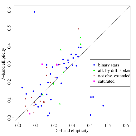
Figure 16: $Y$ and $J$ band ellipticities of sources for which both classifiers disagree; the dotted line is the main diagonal

Comparing our classifier and the UKIDSS pipeline to the Stripe 82 data, Figure 17 shows the mismatch rates of both classifiers, taking the SDSS $r$-band classifications as a reference. To do this we have converted the posterior probabilities into class labels; an object is labelled as a star if $P_{\mathrm{s}}\geq 0.5$, otherwise as a galaxy. We have limited the sources to those with $16<r<20.5$ so as to avoid saturated sources ($r\la 16$) and sources for which the uncertainty of the SDSS labels is non-negligible ($r\ga 20.5$). It is clear that the Bayesian classifier is more accurate than the UKIDSS pipeline classifier; even though the difference in performance decreases for fainter magnitudes. For sources with $16.6\leq Y<17.4$, our classifier achieves a mismatch rate of $0.0154$, compared to $0.0314$ for the UKIDSS pipeline. At the faint end ($Y>20$), the mismatch rates are $0.0679$ (our classifier) and $0.0751$ (UKIDSS pipeline). For all sources with $16<r<20.5$, the mismatch rate for the UKIDSS pipeline ($0.0440$) is more than double that of our classifier ($0.0218$).

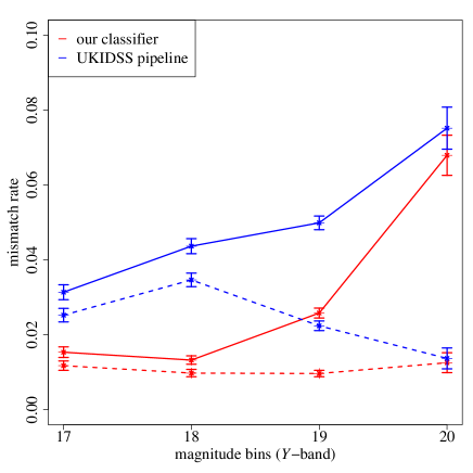
Figure 17: Mismatch rates between the SDSS $r$-band class labels and labels based on our classifier (red) and the UKIDSS pipeline (blue). Mismatch rates are shown both for all sources (with $16<r<20.5$; solid lines) and for those sources for which our classifier outputs very definite classifications ($P_{\mathrm{s}}<0.1$ or $P_{\mathrm{s}}>0.9$; dashed lines). The magnitude values on the horizontal axis are the mid-range values of the bins used to compute the rates. Also shown are the standard errors of the mismatch rates.

6.4 Value of the Bayesian method

The good performance of both the UKIDSS pipeline classifier and our method over the entire sample is unsurprising, as most sources are detected with a sufficient signal–to–noise ratio that they can be classified without effort. However it is often the case that that the most important sources scientifically are those close to any new survey’s detection limit – these objects would not have been detected by shallower surveys in the same band(s) and inevitably dominate the new discoveries from a given data-set. Hence the inclusion of prior information in the Bayesian classifier is most important for just these sources where it results in significant numbers of more accurate classifications.

Our method provides realistic estimates of the classification uncertainties and allows users, by setting constraints on the posterior classification probabilities $P_{\mathrm{s}}$, to specify the completeness (the fraction of target class sources that have actually been selected) and contamination (the fraction of the selected sources which are not from the target class) of a given selection before starting observations. Thus users can design the selection to suit the survey’s aims.

A practical application of our method would be to look at the amount of telescope time that would be required to follow-up a morphologically-selected sample of targets. If one imagines a spectroscopic survey of faint stars, and one was to trust star–galaxy separators such as the ones used by UKIDSS or SDSS versus selecting sources with $P_{\mathrm{s}}>0.9$ from our method, then a certain proportion of telescope time would be spent observing compact / faint galaxies that were misclassified. While there will certainly also be misclassified sources when selecting objects by basing the selection on $P_{\mathrm{s}}$, their proportion can be greatly reduced.

Obviously there is a trade-off between completeness and efficiency when performing source selection. Table 3 lists, for different fluxes, both completeness and efficiency (the fraction of the selected sources which are actually of the target class) for different methods of selecting faint stars, namely selecting sources with $P_{\mathrm{s}}>0.9$ or $P_{\mathrm{s}}>0.5$, using the UKIDSS pipeline single-band or merged class labels, or selecting sources for which the UKIDSS pipeline posterior star probability exceeds $0.9$. While the efficiencies of the different methods are comparable for $Y\simeq 17$ and $Y\simeq 18$, our method leads to better completeness levels at these fluxes (both for using $P_{\mathrm{s}}>0.5$ and $P_{\mathrm{s}}>0.9$). For $Y\simeq 19$ our method with $P_{\mathrm{s}}>0.9$, using the UKIDSS merged class labels and using the UKIDSS pipeline posteriors perform identically. Basing the selection on the UKIDSS $Y$-band class labels or on the posteriors from our method with $P_{\mathrm{s}}>0.5$ leads to higher completeness but lower efficiency (but our method yields a much higher completeness than using the UKIDSS $Y$-band labels and also a marginally larger efficiency). Real differences can, however, be seen at $Y\simeq 20$: while our method with $P_{\mathrm{s}}>0.9$ has a much lower completeness level than the UKIDSS pipeline based methods, it also achieves a much higher efficiency. If telescope time is limited and completeness not important, then basing source selection on $P_{\mathrm{s}}$ can lead to a considerable reduction in ‘wasted’ observation time. Using our method with $P_{\mathrm{s}}>0.5$ leads to completeness and efficiency levels more in line with the UKIDSS pipeline based methods.

Table 3: Completeness (comp.) and efficiency (eff.) for different selection methods at different fluxes. The SDSS Stripe 82 class labels have been taken as reference.

	$16.6<Y<17.4$		$17.6<Y<18.4$		$18.6<Y<19.4$		$19.6<Y<20.4$
	comp.	eff.	comp.	eff.	comp.	eff.	comp.	eff.
our method with $P_{\mathrm{s}}>0.9$	0.980	0.996	0.968	0.993	0.785	0.971	0.103	0.866
our method with $P_{\mathrm{s}}>0.5$	0.984	0.996	0.980	0.992	0.916	0.956	0.540	0.803
UKIDSS $Y$-band class star label $=-1$ (stars)	0.954	0.997	0.900	0.993	0.794	0.945	0.675	0.652
UKIDSS merged class star label $=-1$ (stars)	0.964	0.997	0.922	0.993	0.782	0.972	0.626	0.799
UKIDSS pipeline posterior star probability $>0.9$	0.963	0.997	0.921	0.993	0.782	0.972	0.626	0.799

7 Conclusions

We have developed a Bayesian formalism for star–galaxy classification in optical or NIR surveys that combines the morphological properties of an object (as measured in multiple passbands) with prior knowledge of the star and galaxy populations. A fully Bayesian approach must also include colour information for self-consistency; but, given the aim of combining morphological information correctly, a number of approximations were developed to maximize the influence of the morphological information.

We have demonstrated our method on data from the UKIDSS LAS, combining morphology statistics measured in the $Y$, $J$, $H$ and $K$ bands (or whatever subset of these a source was detected in). The morphology statistic used, ClassStat (Irwin et al., 2010), represents a powerful means of data compression from the full image, and contains almost all the useful information for the faint sources (which are the main motivation for the development of sophisticated star–galaxy classification techniques). However, the existing UKIDSS data products include only heuristic combinations of the band-specific classifications, and the application of the Bayesian method developed here makes it possible to extract all the useful UKIDSS information on a source’s morphology in as self-consistent a manner as is possible without using colour information as well. In particular, the use of prior information avoids the overly-confident classification of faint sources, for which the available measurements contain little morphological information.

Our test sample of UKIDSS LAS sources was chosen to lie in the multiply-scanned SDSS Stripe 82 region, giving us independent and almost totally reliable classifications of all our sources. (This is a rare situation outside simulations, and an opportunity that could be used for a number of similar testing schemes.) Converting the posterior probabilities into class labels, the Bayesian classifier achieves an error rate of $0.068$ at the UKIDSS detection limit, compared to $0.075$ for the UKIDSS pipeline. For all non-saturated sources, the error rate for our model lies at $0.022$, compared to $0.044$ for the UKIDSS pipeline.

The Bayesian model used to separate stars and galaxies described here can be very easily applied to other surveys with similar statistics measuring the extendedness of sources. The multiple advantages of such a classifier (posterior probabilities, use of prior knowledge, rigorous computation of multi-band classifications, ability to cope with missing detections) and its good performance exhibited for the UKIDSS data provide a strong argument in favour of a wider use of this methodology. In particular the use of our method can improve the efficiency of telescope time.

References

- Andreon et al. (2000) Andreon S., Gargiulo G., Longo G., Tagliaferri R., Capuano N., 2000, MNRAS, 319, 700
- Baldry et al. (2010) Baldry I. K., et al., 2010, MNRAS, 404, 86
- Ball et al. (2006) Ball N. M., Brunner R. J., Myers A. D., Tcheng D., 2006, ApJ, 650, 497
- Ball et al. (2004) Ball N. M., Loveday J., Fukugita M., Nakamura O., Okamura S., Brinkmann J., Brunner R. J., 2004, MNRAS, 348, 1038
- Bazell & Miller (2005) Bazell D., Miller D. J., 2005, ApJ, 618, 723
- Bazell & Peng (1998) Bazell D., Peng Y., 1998, ApJS, 116, 47
- Bertin & Arnouts (1996) Bertin E., Arnouts S., 1996, A&AS, 117, 393
- Casali et al. (2007) Casali M., et al., 2007, A&A, 467, 777
- Conover (1999) Conover W., 1999, Practical Nonparametric Statistics, 3rd edn. John Wiley & Sons
- Drinkwater et al. (2003) Drinkwater M. J., Gregg M. D., Hilker M., Bekki K., Couch W. J., Ferguson H. C., Jones J. B., Phillipps S., 2003, Nature, 423, 519
- Dye et al. (2006) Dye S., et al., 2006, MNRAS, 372, 1227
- Fukugita et al. (1996) Fukugita M., Ichikawa T., Gunn J. E., Doi M., Shimasaku K., Schneider D. P., 1996, AJ, 111, 1748
- Hambly et al. (2008) Hambly N. C., et al., 2008, MNRAS, 384, 637
- Hastie et al. (2008) Hastie T., Tibshirani R., Friedman J., 2008, The Elements of Statistical Learning: Data Mining, Inference, and Prediction, 2nd edn. Springer-Verlag
- Hewett et al. (2006) Hewett P. C., Warren S. J., Leggett S. K., Hodgkin S. T., 2006, MNRAS, 367, 454
- Heydon-Dumbleton et al. (1989) Heydon-Dumbleton N. H., Collins C. A., MacGillivray H. T., 1989, MNRAS, 238, 379
- Irwin (1985) Irwin M. J., 1985, MNRAS, 214, 575
- Irwin et al. (2010) Irwin M. J., Lewis J., Hodgkin S. T., Gonzales–Solares 2010, MNRAS, in preparation
- Jarvis & Tyson (1981) Jarvis J. F., Tyson J. A., 1981, AJ, 86, 476
- John (1997) John G. H., 1997, PhD thesis, Stanford University
- Koo & Kron (1982) Koo D. C., Kron R. G., 1982, A&A, 105, 107
- Kron (1980) Kron R., 1980, ApJS, 43, 305
- Lawrence et al. (2007) Lawrence A., et al., 2007, MNRAS, 379, 1599
- Lawrence et al. (2007) Lawrence A., et al., 2007, MNRAS, 379, 1599
- Leauthaud et al. (2007) Leauthaud A., et al., 2007, ApJS, 172, 219
- Lintott et al. (2008) Lintott C. J., et al., 2008, MNRAS, 389, 1179
- Lupton et al. (2001) Lupton R., Gunn J. E., Ivezić Z., Knapp G. R., 2001, in preparation, 0, 1
- MacGillivray et al. (1976) MacGillivray H. T., Martin R., Pratt N., Reddish V., Seddon H., Alexander L., Walker G., Williams P., 1976, MNRAS, 176, 265
- Mähönen & Frantti (2000) Mähönen P., Frantti T., 2000, ApJ, 541, 261
- Messier (1781) Messier C., 1781, Connaissance des Temps, Pour l’Année Commune 1783.. pp 227–267
- Miller & Browning (2003) Miller D. J., Browning J., 2003, Transactions on Pattern Analysis and Machine Intelligence, 25, 1468
- Mortlock et al. (2010) Mortlock D. J., Patel M., Warren S. J., Hewett P. C., Venemans B. P., McMahon R. G., 2010, MNRAS, submitted
- Odewahn et al. (1992) Odewahn S. C., Stockwell E. B., Pennington R. L., Humphreys R. M., Zumach W. A., 1992, AJ, 103, 318
- Philip et al. (2002) Philip N. S., Wadadekar Y., Kembhavi A., Joseph K. B., 2002, A&A, 385, 1119
- Richards et al. (2004) Richards G. T., et al., 2004, ApJS, 155, 257
- Schwarz (1978) Schwarz G., 1978, The Annals of Statistics, 6, 461
- Scranton et al. (2005) Scranton R., Connolly A. J., Szalay A. S., Lupton R. H., Johnston D., Budavari T., Brinkman J., Fukugita M., 2005, AJ, submitted
- Scranton et al. (2002) Scranton R., et al., 2002, ApJ, 579, 48
- Sebok (1979) Sebok W. L., 1979, AJ, 84, 1526
- Sérsic (1963) Sérsic J. L., 1963, Boletin de la Asociacion Argentina de Astronomia La Plata Argentina, 6, 41
- Shapiro & Wilk (1965) Shapiro S., Wilk M., 1965, Biometrika, 52, 591
- Skrutskie et al. (2006) Skrutskie M. F., et al., 2006, AJ, 131, 1163
- Suchkov et al. (2005) Suchkov A. A., Hanisch R. J., Margon B., 2005, AJ, 130, 2439
- Warren et al. (2007) Warren S. J., et al., 2007, MNRAS, 375, 213
- Weir et al. (1995) Weir N., Fayyad U. M., Djorgovski S., 1995, AJ, 109, 2401
- Wolf et al. (2001) Wolf C., Meisenheimer K., Röser H.-J., 2001, A&A, 365, 660
- Yasuda et al. (2001) Yasuda N., et al., 2001, AJ, 122, 1104
- York et al. (2000) York D. G., et al., 2000, AJ, 120, 1579