Hydrodynamic effects on concentration fluctuations in multicomponent membranes

Abstract

We investigate the hydrodynamic effects on the dynamics of critical concentration fluctuations in multicomponent fluid membranes. Two geometrical cases are considered; (i) confined membrane case and (ii) supported membrane case. We numerically calculate the wavenumber dependence of the effective diffusion coefficient by changing the temperature and/or the thickness of the bulk fluid. For some limiting cases, the result is compared with the previously obtained analytical expression. An analogy of the multicomponent membrane to 2D microemulsion is explored for the confined membrane geometry.

I Introduction

Biomembranes can be regarded as multipurpose envelopes fundamental to the very existence of life. Composed of a huge variety of amphiphilic molecules, this approximately 5 nm thick quasi-two-dimensional fluid sheet separates the inner and outer environments of the cells and organelles alberts . Apart from delineating the cell and organelle boundaries, membranes also play a significant role in a variety of physiological functions such as trans-membrane transport of materials and cell signaling alberts .

Biomembranes have attracted renewed interests in the context of the lipid “raft” hypothesis proposed a little over a decade ago simons-97 . These 10–100 nm sized lipid domains with higher concentrations of cholesterol were proposed to play a significant role in regulating certain cellular functions simons-97 ; edidin-03 ; hancock-06 . Recent experiments using the stimulated emission depletion (STED) microscopy on plasma membranes in vivo narrowed the size-range of the rafts to 10–20 nm eggeling-09 . Despite extensive studies in this area, the details of the underlying physical mechanisms leading to formation of rafts, their stability, and the regulation of the finite domain size remain elusive and controversial munro-03 ; shaw-06 .

Although the biological significance of rafts is still under debate, there is no doubt about the rich physics and chemistry that have been uncovered by the membrane studies to examine the raft hypothesis. Numerous experiments on intact cells and artificial membranes containing saturated lipids, unsaturated lipids and cholesterol have demonstrated the segregation of lipids into liquid-ordered (${\rm L_{o}}$) and liquid-disordered (${\rm L_{d}}$) phases below the miscibility transition temperature veatch-03 ; veatch-05 . The ${\rm L_{o}}$-phase is usually rich in saturated lipids and cholesterol. Below the transition temperature, the domains undergo coarsening with the largest domain limited by the system size veatch-05 . The primary driving force for the domain coarsening is due to the positive line tension at the domain boundaries. Studies on the diffusion of domains cicuta-07 and on the dynamics of domain coarsening saeki-06 ; yanagisawa-07 ; veatch-07 have been reported.

Recently, studies on multicomponent membranes above the transition temperature have also gained much attention. As the critical point is approached from above, one observes composition fluctuations spanning a wide range of length and time scales sengers-86 . Veatch et al. made a notable attempt to investigate critical fluctuations in lipid mixtures veatch-07 . Deuterium NMR experiments on model ternary membranes composed of dioleoylphosphatidylcholine (DOPC), dipalmitoylphosphatidylcholine (DPPC) and cholesterol were used to construct the ternary phase diagram. With the determination of the line of miscibility critical points, they observed that the NMR resonances were broadened in the vicinity of the critical points. Such a spectral broadening was attributed to the compositional fluctuations in the membrane having spatial dimensions less than 50 nm.

A more quantitative analysis of the critical fluctuations using fluorescence microscopy was addressed by Honerkamp-Smith et al. for ternary mixtures of DPPC, diphytanoylphosphatidylcholine (diPhyPC) and cholesterol hsmith-08 . When the critical temperature $T_{\rm c}$ is approached from above, the correlation length diverges according to $\xi\approx|T-T_{\rm c}|^{-\bar{\nu}}$ where $\bar{\nu}$ is the critical exponent and $T$ the temperature. (In order to prevent the confusion with the notations used later, the critical exponents are written with a bar.) When $T_{\rm c}$ is approached from below, on the other hand, the order parameter given by the difference in lipid compositions vanishes as $\delta\psi\approx(T_{\rm c}-T)^{\bar{\beta}}$. From the measurements of the critical exponents $\bar{\nu}$ and $\bar{\beta}$, the authors concluded that the critical behavior in ternary membranes is in the universality class of the 2D Ising model onsager-44 . Later, it was also shown that giant plasma membrane vesicles extracted from that of living rat basophil leukemia cells exhibit a critical behavior veatch-08 . These experimental observations suggest that lateral heterogeneity present in real cell membranes at physiological conditions correspond to critical fluctuations hsmith-08 ; veatch-08 . In other words, concentration fluctuations above the transition temperature (rather than below) can also be responsible for raft structures in cell membranes.

There have also been several theoretical works on concentration fluctuations in multicomponent membranes. Using renormalization group techniques, Tserkovnyak and Nelson calculated protein diffusion in a multicomponent membrane close to a rigid substrate Tserkovnyak-06 . They pointed out that, in the vicinity of the critical point, the effective protein diffusion coefficient acquires a power-law behavior. Seki et al. reported equivalent results with the use of a two-dimensional (2D) hydrodynamic model involving a phenomenological momentum decay mechanism seki-07 . Later Haataja showed that the effective diffusion coefficient exhibits a crossover from a logarithmic behavior to an algebraic dependence for larger length scales haataja-09 . In his theory, an approximate empirical relation for the diffusion coefficient of a moving object was employed petrov-08 . A rigorous hydrodynamic calculation performed by Inaura and Fujitani arrived at similar results inaura-08 .

The present article uses the idea of critical phenomena to calculate the effective diffusion coefficient in multicomponent lipid membranes. Based on the time-dependent Ginzburg-Landau approach with full hydrodynamics, we calculate in particular the decay rate of the concentration fluctuations occurring in membranes. We deal with the case where the membrane is surrounded by a bulk solvent and two walls as depicted in Fig. 1. Such a situation is worth considering because biological membranes interact strongly with other cells, substrates or even the underlying cytoskeleton which affects the structural and transport properties of the membrane simons-04 . We note that effects of the substrates on the diffusion coefficient of proteins have been investigated before evans-88 ; stone-98 . Two surrounding geometries of the membrane are discussed; (i) confined membrane and (ii) supported membrane. We also study the situation when the multicomponent membranes form 2D microemulsions gompper-schick . This interesting viewpoint is motivated by a recent work which predicts the reduction of the line tension in membranes containing saturated, unsaturated and hybrid lipids (one tail saturated and the other unsaturated) brewster-09 ; brewster-10 . Based on chain entropy arguments, they proposed that hybrid lipids in 2D play an equivalent role to surfactant molecules in three-dimensions (3D). Hence we shall explore the concentration fluctuations in 2D microemulsion.

This paper is organized as follows. In Section II, we first obtain the membrane mobility tensors that are used in the subsequent calculations. In Section III, the decay rates of concentration fluctuations are analyzed for confined and supported membrane cases. Section IV deals with the microemulsion picture of the multicomponent membranes. Finally we close with some discussions in Section V.

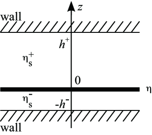
Figure 1: Schematic picture showing a planar liquid membrane having 2D viscosity $\eta$ located at $z=0$. It is sandwiched by a solvent of 3D viscosity $\eta_{\rm s}^{\pm}$. Two impenetrable walls are located at $z=\pm h^{\pm}$ bounding the solvent.

II Membrane hydrodynamics

In this section, we start with the membrane equations of motion as well as the requisite membrane mobility tensors for the two geometries. The membrane is assumed to be an infinite planar sheet of liquid and its out-of-plane fluctuations are totally neglected, which is justified for typical bending rigidities of bilayers. The liquid membrane, fixed in the $xy$-plane at $z=0$, is embedded in a bulk fluid such as water or solvent that is further bounded by hard walls as shown in Fig. 1. The upper ($z>0$) and the lower ($z<0$) fluid regions are denoted by $``+"$ and $``-"$, respectively. Since the 3D viscosities of the upper and the lower solvent can be different, we denote them as $\eta_{\rm s}^{\pm}$. Consider the situation in which impenetrable walls are located at $z=\pm h^{\pm}$, where $h^{+}$ and $h^{-}$ can also be different in general.

Let ${\bf v}({\bf r})$ be the 2D velocity of the membrane fluid. The 2D vector ${\bf r}=(x,y)$ represents a point in the plane of the membrane which is assumed to be incompressible

$$\nabla\cdot{\bf v}=0.$$ (1)

Here $\nabla$ is a 2D differential operator. We work in the low-Reynolds number regime of the membrane hydrodynamics so that the inertial effects can be neglected. This allows us to use the 2D Stokes equation given by

$$\eta\nabla^{2}{\bf v}-\nabla p+{\bf f}_{\rm s}+\bf{F}=0,$$ (2)

where $\eta$ is the 2D membrane viscosity, $p$ the 2D in-plane pressure, ${\bf f}_{\rm s}$ the force exerted on the membrane by the surrounding fluid (“s” stands for the solvent), and ${\bf F}$ is any other force acting on the membrane.

Once we know ${\bf f}_{\rm s}$, the membrane velocity can be obtained from eqn (2) as

$${\bf v}[{\bf q}]={{\bf G}}[{\bf q}]\cdot{\bf F}[{\bf q}],$$ (3)

where ${\bf v}[{\bf q}]$, ${\bf G}[{\bf q}]$ and ${\bf F}[{\bf q}]$ (${\bf q}=(q_{x},q_{y})$) are the Fourier components of ${\bf v}({\bf r})$, ${\bf G}({\bf r})$ and ${\bf F}({\bf r})$ defined by

$${\bf v}({\bf r})=\int\frac{{\rm d}{\bf q}}{(2\pi)^{2}}{\bf v}[{\bf q}]\exp(i{\bf q}\cdot{\bf r}),$$ (4)

$${\bf G}({\bf r})=\int\frac{{\rm d}{\bf q}}{(2\pi)^{2}}{\bf G}[{\bf q}]\exp(i{\bf q}\cdot{\bf r}),$$ (5)

and

$${\bf F}({\bf r})=\int\frac{{\rm d}{\bf q}}{(2\pi)^{2}}{\bf F}[{\bf q}]\exp(i{\bf q}\cdot{\bf r}),$$ (6)

respectively. Using the stick boundary conditions at $z=0$ and $z=\pm h^{\pm}$, we can solve the hydrodynamic equations to obtain ${\bf f}_{\rm s}$ sanoop-poly-10 . Its perpendicular component with respect to ${\bf q}$ is given by

$$f_{\rm s\perp}[{\bf q}]=-\eta_{\rm s}^{+}v_{\perp}q\coth(qh^{+})-\eta_{\rm s}^{-}v_{\perp}q\coth(qh^{-}),$$ (7)

where $q=|{\bf q}|$ and $v_{\perp}$ is also the perpendicular component of ${\bf v}$ with respect to ${\bf q}$. On the other hand, one can show that the parallel component of ${\bf f}_{\rm s}$ is zero. After some calculations, the components of the mobility tensor ${\bf G}[{\bf q}]$ finally becomes

$$G_{\alpha\beta}[{\bf q}]= \frac{1}{\eta q^{2}+q[\eta_{\rm s}^{+}\coth(qh^{+})+\eta_{\rm s}^{-}\coth(qh^{-})]}$$

$$\times\left(\delta_{\alpha\beta}-\frac{q_{\alpha}q_{\beta}}{q^{2}}\right),$$ (8)

with $\alpha,\beta=x,y$. The full details of the calculation are given in the separate article by Ramachandran et al. sanoop-poly-10 .

As in ref. inaura-08 , we first consider the case when the two walls are located at equal distances from the membrane, i.e., $h^{+}=h^{-}=h$. Then the above mobility tensor simplifies to

$$G_{\alpha\beta}[{\bf q}]=\frac{1}{\eta[q^{2}+\nu q\coth(qh)]}\left(\delta_{\alpha\beta}-\frac{q_{\alpha}q_{\beta}}{q^{2}}\right),$$ (9)

where $\nu\equiv 2\eta_{\rm s}/\eta$ with $\eta_{\rm s}=(\eta_{\rm s}^{+}+\eta_{\rm s}^{-})/2$. This expression, taken in the limit of large $h$, has been used previously in calculating the correlated diffusion coefficients of particles embedded in a membrane oppenheimer-09 .

For supported membranes, $h^{+}$ is infinitely large while $h^{-}$ is finite when compared to the membrane thickness. In this case, eqn (8) reduces to sanoop-poly-10

$$G_{\alpha\beta}[{\bf q}]=\frac{1}{\eta[q^{2}+\nu q(1+\coth(qh^{-}))/2]}\left(\delta_{\alpha\beta}-\frac{q_{\alpha}q_{\beta}}{q^{2}}\right).$$ (10)

This equation has been used for the investigation of the correlated dynamics of inclusions in a supported membrane oppenheimer-10 .

III Dynamics of concentration fluctuations

In order to discuss the dynamics of concentration fluctuations above the transition temperature, we closely follow the formalism used in ref. nonomura-99 . Here we extend our previous work in ref. seki-07 for membranes embedded in a solvent confined by two walls (confined membrane) or supported on a substrate (supported membrane).

Consider a two-component fluid membrane composed of lipid A and lipid B whose local area fractions are denoted by $\phi_{\rm A}({\bf r})$ and $\phi_{\rm B}({\bf r})$, respectively. Since the relation $\phi_{\rm A}({\bf r})+\phi_{\rm B}({\bf r})=1$ holds, we introduce a new variable defined by $\psi({\bf r})\equiv\phi_{\rm A}({\bf r})-\phi_{\rm B}({\bf r})$. The simplest form of the free energy functional ${\mathcal{F}}\{\psi\}$ describing the fluctuation around the homogeneous state is

$${\mathcal{F}}\{\psi\}=\int{\rm d}{\bf r}\left[\frac{a}{2}\psi^{2}+\frac{c}{2}(\nabla\psi)^{2}-\mu\psi\right],$$ (11)

where $a>0$ is proportional to the temperature difference from the critical temperature, $c>0$ is related to the line tension and $\mu$ is the chemical potential.

The time evolution of concentration in the presence of hydrodynamic flow is given by the time-dependent Ginzburg-Landau equation for a conserved order parameter nonomura-99

$$\frac{\partial\psi}{\partial t}+\nabla\cdot({\bf v}\psi)=L\nabla^{2}\frac{\delta{\mathcal{F}}}{\delta\psi},$$ (12)

where $L$ is the kinetic coefficient. In the membrane hydrodynamic equation (2), on the other hand, we need to incorporate the thermodynamic force due to the concentration fluctuations. Hence we have

$$\bf{F}=-\psi\nabla\frac{\delta{\mathcal{F}}}{\delta\psi}.$$ (13)

We implicitly assumed that the relaxation of the velocity ${\bf v}$ is much faster than that of concentration $\psi$ seki-07 . The membrane velocity can be formally solved using the appropriate 2D mobility tensor $G_{\alpha\beta}({\bf r},{\bf r}^{\prime})$ derived in the previous section,

$$v_{\alpha}({\bf r},t)=\int{\rm d}{\bf r}^{\prime}G_{\alpha\beta}({\bf r},{\bf r}^{\prime})(\nabla_{\beta}^{\prime}\psi)\frac{\delta{\mathcal{F}}}{\delta\psi({\bf r}^{\prime})}.$$ (14)

Since our interest is in the concentration fluctuations around the homogeneous state, we define $\delta\psi({\bf r},t)=\psi({\bf r},t)-\bar{\psi}$, where the bar indicates the spatial average. The free energy functional expanded in powers of $\delta\psi$ becomes,

$${\mathcal{F}}\{\delta\psi\}=\int{\rm d}{\bf r}\left[\frac{a}{2}(\delta\psi)^{2}+\frac{c}{2}(\nabla\delta\psi)^{2}\right].$$ (15)

Substituting eqn (14) into eqn (12), we get

$$\frac{\partial\delta\psi({\bf r},t)}{\partial t}=L\nabla^{2}\frac{\delta{\mathcal{F}}}{\delta(\delta\psi)}$$

$$-\int{\rm d}{\bf r}^{\prime}(\nabla_{\alpha}\delta\psi({\bf r}))G_{\alpha\beta}({\bf r},{\bf r}^{\prime})(\nabla_{\beta}^{\prime}\delta\psi({\bf r}^{\prime}))\frac{\delta{\mathcal{F}}}{\delta(\delta\psi({\bf r}^{\prime}))}.$$ (16)

We now consider the dynamics of the time-correlation function defined by

$$S({\bf r},t)=\langle\delta\psi({\bf r}_{1},t)\delta\psi({\bf r}_{2},0)\rangle,$$ (17)

where ${\bf r}={\bf r}_{2}-{\bf r}_{1}$. Within the factorization approximation nonomura-99 , the spatial Fourier transform of $S({\bf r},t)$ defined by

$$S({\bf r},t)=\int\frac{{\rm d}{\bf q}}{(2\pi)^{2}}S[{\bf q},t]\exp(i{\bf q}\cdot{\bf r}),$$ (18)

satisfies the following equation

$$\frac{\partial S[{\bf q},t]}{\partial t}=-\left(\Gamma^{(1)}[{\bf q}]+\Gamma^{(2)}[{\bf q}]\right)S[{\bf q},t].$$ (19)

In the above, the first term $\Gamma^{(1)}[{\bf q}]$ denotes the van Hove part of the relaxation rate given by

$$\Gamma^{(1)}[{\bf q}]=Lk_{\rm B}Tq^{2}\chi^{-1}[{\bf q}].$$ (20)

Here the static correlation function is defined by

$$\chi[{\bf q}]=\langle\delta\psi[{\bf q}]\delta\psi[-{\bf q}]\rangle=\frac{k_{\rm B}T}{c(q^{2}+\xi^{-2})},$$ (21)

where $\xi\equiv(c/a)^{1/2}$ is the correlation length, $k_{\rm B}$ the Boltzmann constant, and $T$ the temperature.

As for the second term in eqn (19), $\Gamma^{(2)}[{\bf q}]$ denotes the hydrodynamic part of the decay rate

$$\Gamma^{(2)} [{\bf q}]=\frac{1}{\chi[{\bf q}]}\int\frac{{\rm d}{\bf p}}{(2\pi)^{2}}q_{\alpha}G_{\alpha\beta}[{\bf p}]q_{\beta}\chi[{\bf q}+{\bf p}],$$ (22)

where either eqn (9) or eqn (10) will be used for the mobility tensor $G_{\alpha\beta}$.

III.1 Confined membrane

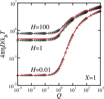
Figure 2: Scaled effective diffusion coefficient $D$ as a function of $Q$ for $H=0.01,1,100$ when $X=1$ for the confined membrane case. The numerically calculated points are joined by lines for clarity. The solid red lines are from the analytical expression given in eqn (26) obtained in the limit of small $H$.

First we consider the situation in which the membrane is confined by two walls which are located at equidistant $h$ from the membrane. The appropriate form of the mobility tensor is given by eqn (9). Substituting it into eqn (22), the hydrodynamic part of the decay rate is expressed as

$$\Gamma^{(2)}[{\bf q}]=\frac{k_{\rm B}T}{\eta\chi[{\bf q}]}\int\frac{{\rm d}{\bf p}}{(2\pi)^{2}}$$

$$\times\frac{\chi[{\bf p}]}{|{\bf p}-{\bf q}|^{2}+\nu|{\bf p}-{\bf q}|\coth(|{\bf p}-{\bf q}|h)}\frac{q^{2}p^{2}-({\bf q}\cdot{\bf p})^{2}}{|{\bf p}-{\bf q}|^{2}}.$$ (23)

We introduce an effective diffusion coefficient $D[{\bf q}]$ (due only to the hydrodynamic effect) defined by

$$\Gamma^{(2)}[{\bf q}]=q^{2}D[{\bf q}].$$ (24)

In order to deal with dimensionless quantities, we rescale all the lengths by the hydrodynamic screening length $\nu^{-1}=\eta/(2\eta_{\rm s})$ such that $P\equiv p/\nu$, $Q\equiv q/\nu$, $X\equiv\xi\nu$ and $H\equiv h\nu$. Then $D[{\bf q}]$ can be rewritten as

$$D[Q;X,H]=\frac{k_{\rm B}T}{4\pi^{2}\eta}(1+Q^{2}X^{2})$$

$$\times\int_{0}^{\infty}{\rm d}P\int_{0}^{2\pi}{\rm d}\theta\frac{P^{3}\sin^{2}\theta}{(1+P^{2}X^{2})[G^{2}+G^{3/2}\coth(\sqrt{G}H)]},$$ (25)

with $G=P^{2}+Q^{2}-2PQ\cos\theta$. Since this integral cannot be performed analytically, we evaluate it numerically. We explore the dependencies of $D$ on the variable $Q$, and the parameters $X$ and $H$.

In Fig. 2, we plot the diffusion coefficient $D$ (scaled by $k_{\rm B}T/4\pi\eta$) as a function of dimensionless wavenumber $Q$ for different solvent thickness $H$ while the correlation length is fixed to $X=1$ (i.e., fixed temperature). In the limit of $Q\ll 1$, $D$ is almost a constant. The calculated $D$ starts to increase around $Q\approx 1$ and a logarithmic behavior (extracted via numerical fitting) is seen for $Q\gg 1$. This trend has been previously reported by Seki et al. seki-07 or Inaura and Fujitani inaura-08 . When $H$ is small such as $H=0.01$, the value of $D$ decreases by one order of magnitude compared to $H=100$. Figure 3 shows the diffusion coefficient $D$ as a function of wave number $Q$ for different $X$ (i.e., different temperature) while the solvent height is fixed to $H=1$. Again, $D$ is nearly constant for $Q\ll 1$, and follows an $S$-shaped curve with increasing $Q$. Finally, a logarithmic dependence is observed from numerical fitting. We note that the above logarithmic behavior for $Q\gg 1$ is in contrast to that of 3D critical fluids as given by the Kawasaki function which increases linearly with $q$ kawasaki-70 .

Figure 3: Scaled effective diffusion coefficient $D$ as a function of $Q$ for $X=0.01,1,100$ when $H=1$ for the confined membrane case.

In Fig. 4, we explore the effect of the correlation length $X$ on $D$ for different values of $H$ when $Q=10^{-3}$. The quantity $X$ measures an effective size of the correlated region formed transiently in the membrane due to thermal fluctuations. When $X\ll 1$, the diffusion coefficient $D$ decreases only logarithmically, which is typical for a pure 2D system saffman-75 ; saffman-76 ; hughes-81 . When $X\gg 1$, on the other hand, the behavior of $D$ depends on the value of $H$. The proximity to the walls results in a loss of momentum from the membrane seki-07 ; sanoop-poly-10 ; diamant-09b . This leads to a rapid suppression of the velocity field within the membrane such that the concentration fluctuations decay slowly. Consequently, the values of $D$ are lower for smaller $H$. The flattening of the curves for large $X$ is due to the dominance of the $X^{2}$ terms in the numerator and denominator of eqn (25). In Fig. 5, we plot $D$ as a function of $H$ for different values of $X$ when $Q=10^{-3}$. In general, there is a monotonic increase in $D$ with larger $H$ followed by a saturation to a constant value. We see that the effect of $H$ is most prominent for large $X$ (close to the critical point), while there is only a weak dependence for $X\ll 1$ (far from the critical point). The former reflects the fact that the membrane fluid is affected by the the outer environment when the correlation length $\xi$ is larger than the hydrodynamic screening length $\nu^{-1}$ i.e, $X\gg 1$ sanoop-poly-10 . For correlation lengths smaller than the $\nu^{-1}$, the outer environment surrounding the membrane is less important. In this situation, the system behaves essentially as a pure 2D one. When the correlation length becomes larger than $\nu^{-1}$, as is the case near the critical point, the outer environment significantly affects membrane dynamics.

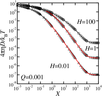
Figure 4: Scaled effective diffusion coefficient $D$ as a function of $X$ for $H=0.01,1,100$ when $Q=10^{-3}$ for the confined membrane case. The solid red lines are from the analytical expression given in eqn (26) obtained in the limit of small $H$.

Figure 5: Scaled effective diffusion coefficient $D$ as a function of $H$ for $X=0.01,1,100$ when $Q=10^{-3}$ for the confined membrane case.

For small $h$, the $\nu q\coth(qh)$ term in the mobility tensor eqn (9) can be replaced by a constant $\nu/h$. In this case, Seki et al. obtained an analytical expression for the effective diffusion coefficient seki-07 . Their result in terms of the dimensionless quantities $Q$, $X$ and $H$ can be reproduced as

$$D[Q;X,H]=\frac{k_{\rm B}T}{4\pi\eta}\frac{1+Q^{2}X^{2}}{2Q^{2}X^{2}}\left[-\ln\left(\frac{X}{\sqrt{H}}\right)\right.$$

$$+\frac{H}{X^{2}}(1+Q^{2}X^{2})\ln\left(\frac{X}{\sqrt{H}(1+Q^{2}X^{2})}\right)$$

$$\left.+\frac{H\Omega}{2X^{2}}\ln\left(\frac{Q_{+}^{4}+Q_{-}^{2}+Q_{+}^{2}\Omega}{\Omega-Q_{-}^{2}-1}\right)\right],$$ (26)

where

$$\Omega=\sqrt{\left(Q^{2}X^{2}+X^{2}/H-1\right)^{2}+4Q^{2}X^{2}},$$ (27)

and

$$Q_{\pm}=\sqrt{Q^{2}X^{2}\pm X^{2}/H}.$$ (28)

Equation (26) is plotted using red curves in Fig. 2 for $H=0.01$ and $1$ with $X=1$. For $H=0.01$, the analytical and numerical data coincide giving credence to accuracy of the numerical solutions. It is seen that even for $H=1$ the agreement is still acceptable. For $H=100$, however, a significant deviation is observed (not shown), which is expected as this limit is beyond the valid range of eqn (26).

The red curves in Fig. 4 also represent the analytical result of eqn (26). It is seen that the analytical and the numerical data points almost coincide for $H=0.01$ and $H=1$. For $H=100$, there is significant deviation from the numerical data (not shown). However, the agreement between the numerical result and the analytical expression is beyond the expected range of $H\ll 1$ and reaches up to $H\approx 1$, as pointed out by Stone and Ajdari stone-98 . Hence eqn (26) can be useful in analyzing the experimental data in many situations.

III.2 Supported membrane

Figure 6: Scaled effective diffusion coefficient $D$ as a function of $Q$ for $H^{-}=0.01,1,100$ when $X=1$ for the supported membrane case plotted with filled symbols. For comparison, the data in Fig. 2 are also plotted with open symbols.

Apart from studying membrane dynamics on vesicles, experiments are also conducted on supported membranes which have a benefit of avoiding curvature effects kaizuka-04 . We proceed now to calculate concentration fluctuations for the supported membrane case. As given by eqn (10), the mobility tensor of a supported membrane is slightly modified from that of a confined membrane. By substituting eqn (10) into eqn (22), we obtain the expression for the effective diffusion coefficient as

$$D[Q;X,H^{-}]=\frac{k_{\rm B}T}{4\pi^{2}\eta}(1+Q^{2}X^{2})\int_{0}^{\infty}{\rm d}P\int_{0}^{2\pi}{\rm d}\theta$$

$$\times\frac{P^{3}\sin^{2}\theta}{(1+P^{2}X^{2})[G^{2}+G^{3/2}(1+\coth(\sqrt{G}H^{-}))/2]},$$ (29)

where $H^{-}\equiv h^{-}\nu$ and $G=P^{2}+Q^{2}-2PQ\cos\theta$ as before.

Performing numerical integrations, we plot in Fig. 6 the effective diffusion coefficient $D$ as a function of $Q$ for different values of $H^{-}$ when $X=1$ (closed symbols). In general, the behavior of $D$ is similar to that of the confined membrane case. When $H^{-}\ll 1$, the calculated $D$ is slightly larger than the confined membrane compared with the same value of $H$. This is because the supported membrane is subjected to only one wall, while the confined membrane is sandwiched by two walls on both sides. The confined and the supported membranes show an almost identical behavior when both $H$ and $H^{-}$ are large enough, as it should be. The other dependencies of $D$ are similar to the confined membrane case except for a slight increase at small $H^{-}$ values.

IV Membrane as a 2D microemulsion

The role of surfactant molecules in 3D microemulsions is to reduce the surface tension at the interface between oil and water. In an analogy to 3D microemulsions, hybrid lipids (one chain unsaturated and the other saturated) act as lineactant molecules which stabilize finite sized domains in 2D. In other words, hybrid lipids play a similar role to surfactant molecules at the interface between ${\rm L_{o}}$ and ${\rm L_{d}}$ domains. It should be also noticed that hybrid lipids form a major percentage of all naturally existing lipids vandeenen-71 ; vanmeer-08 . Based on a simple model of hybrid lipids, Brewster et al. showed that finite sized domains can be formed in equilibrium brewster-09 ; brewster-10 . A subsequent model predicted stabilized domains even in a system of saturated/hybrid/cholesterol lipid membranes yamamoto-10 . Being motivated by this idea, we calculate the decay rate of concentration fluctuations when the free energy of the multicomponent membrane has the form of a 2D microemulsion. Here we consider only the confined membrane geometry, and use eqn (9) for the mobility tensor.

The free energy functional for a microemulsion includes a higher order derivative term and is expressed in terms of $\delta\psi$ as gompper-schick

$${\mathcal{F}}_{\rm ME}\{\delta\psi\}=\int{\rm d}{\bf r}\left[\frac{a}{2}(\delta\psi)^{2}+\frac{c}{2}(\nabla\delta\psi)^{2}+\frac{g}{2}(\nabla^{2}\delta\psi)^{2}\right],$$ (30)

with $a,g>0$ and $c<0$. The negative value of $c$ creates 2D interfaces, while the term with positive $g$ is a stabilizing term. This form of the free energy has been used previously to study coupled modulated bilayers hirose-09 . As in the previous section, the decay rate of the correlation function can be split into two parts. First, the van Hove part becomes now

$$\Gamma^{(1)}_{\rm ME}[{\bf q}]=Lk_{\rm B}Tq^{2}\chi^{-1}_{\rm ME}[{\bf q}],$$ (31)

where $L$ is the kinetic coefficient assumed to be same as before, and the static correlation function $\chi_{\rm ME}[{\bf q}]$ is strey-87

$$\chi_{\rm ME}[{\bf q}]=\frac{k_{\rm B}T}{gq^{4}+cq^{2}+a}.$$ (32)

By defining

$$q_{0}^{2}=-\frac{c}{2g},$$ (33)

$$\sigma^{4}=\frac{a}{g}-\left(\frac{c}{2g}\right)^{2},$$ (34)

the static correlation function can be also written as

$$\chi_{\rm ME}[{\bf q}]=\frac{k_{\rm B}T}{g\left[(q^{2}-q_{0}^{2})^{2}+\sigma^{4}\right]}.$$ (35)

On plotting $\chi_{\rm ME}$ as a function of $q$, a peak appears at $q=q_{0}$ followed by a $q^{-4}$-decay. The width of the peak is given by $\sigma$, and a lamellar phase appears when $\sigma=0$. Notice that $c=0$ is called the Lifshitz point at which the peak occurs for $q=0$ gompper-90 . Using the form of eqn (35), we can rewrite eqn (31) as

$$\Gamma^{(1)}_{\rm ME}[{\bf q}]=Lgq^{2}\left[(q^{2}-q_{0}^{2})^{2}+\sigma^{4}\right].$$ (36)

Figure 7: Scaled effective diffusion coefficient $D_{\rm ME}$ as a function of $Q$ for $H=0.01,1,100$ when $Q_{0}=\Sigma=1$ for the confined membrane case.

As in the previous section, we next write the hydrodynamic part of the decay rate in terms of the effective diffusion coefficient $D_{\rm ME}[{\bf q}]$ as

$$\Gamma^{(2)}_{\rm ME}[{\bf q}]=q^{2}D_{\rm ME}[{\bf q}].$$ (37)

Using eqn (9) for the mobility tensor, we obtain $D_{\rm ME}$ as

$$D_{\rm ME}[Q;Q_{0},\Sigma,H]=\frac{k_{\rm B}T}{4\pi^{2}\eta}[(Q^{2}-Q_{0}^{2})^{2}+\Sigma^{4}]\int_{0}^{\infty}{\rm d}P$$

$$\times\int_{0}^{2\pi}{\rm d}\theta\frac{P^{3}\sin^{2}\theta}{[(P^{2}-Q_{0}^{2})^{2}+\Sigma^{4}][G^{2}+G^{3/2}\coth(\sqrt{G}H)]},$$ (38)

where $P\equiv p/\nu$, $Q\equiv q/\nu$, $Q_{0}\equiv q_{0}/\nu$, $\Sigma\equiv\sigma/\nu$, $H\equiv h\nu$, and $G=P^{2}+Q^{2}-2PQ\cos\theta$.

In Fig. 7, we plot $D_{\rm ME}$ as a function of $Q$ for different values of $H$ when $Q_{0}=\Sigma=1$ are fixed. When $Q\ll 1$, $D$ shows a constant value. We also observe the 2D characteristic of logarithmic behavior of $D$ for $Q\gg 1$. For $Q\ll 1$, the effect of the outer environment is felt with the suppression of the diffusion coefficient with smaller $H$. The curves almost overlap when $Q\gg 1$ indicating the negligible effect of the outer environment at large wave numbers. An interesting feature of $D_{\rm ME}$ is the dip occurring at $Q\approx Q_{0}$ which does not exist for binary critical fluids. This can be attributed to the peak at $q=q_{0}$ in $\chi_{\rm ME}[{\bf q}]$ nonomura-99 ; strey-87 ; hennes-94 . For 3D microemulsions, however, it is known that the effective diffusion coefficient varies linearly with $q$ for large wave numbers nonomura-99 .

Although the analogy between a 3D and 2D microemulsion has been invoked, it should be pointed out that a 3D microemulsion formed from an oil/water/surfactant mixture arises predominantly due to the differences in relative affinity between the components. For the 2D case, it is the physical interactions from the hydrocarbon chain packing requirements at the ${\rm L_{o}}$/${\rm L_{d}}$ interface that gives rise to the lineactant properties of the hybrid lipid.

V Discussion

In summary, we have calculated the decay rate of concentration fluctuations in a multicomponent fluid membrane for two geometries. First we considered the membrane surrounded by solvent of finite depth which is further bounded by two walls. In the second geometry, we allow the solvent depth on one side of the membrane to be infinitely large. This is equivalent to a supported membrane in experimental situations. The resulting integrals for the effective diffusion coefficient of the concentration fluctuations are calculated numerically to determine the various dependencies. We have also explored a possibility of considering the multicomponent membrane as a 2D microemulsion.

The present work follows Seki et al. who were able to use analytical means to obtain the effective diffusion coefficient seki-07 . Although their result should be valid only in the limit of very small $h$, the agreement between the numerical result and the analytical expression is fairly well as long as $h\leq\nu^{-1}$. The opposite limit of very large $h$ was studied by Inaura and Fujitani through numerical methods inaura-08 . Using the general mobility tensor given by eqn (8), we are able to probe all the intermediate situations of finite $h$. We have verified that our results properly interpolates between these previous works in the limits of $H\to 0$ and $H\to\infty$.

In our case, the measure of the size of the transient structures is given by the correlation length $\xi$. Close to the critical point, $\xi$ diverges and the hydrodynamic effects of the outer fluid play a significant role in altering the diffusion coefficient. It has been previously shown through explicit calculations that the diffusion coefficient has a logarithmic behavior $D\approx\ln(1/R)$ when the size of the diffusing object $R$ is less than the hydrodynamic screening length, i.e., $R\ll\nu^{-1}$ saffman-75 ; saffman-76 . When $R\gg\nu^{-1}$, on the other hand, the fluid flow in the bulk leads to the diffusion coefficient to show $1/R$-behavior (this condition occurs when there are no walls) hughes-81 . In the presence of walls or a substrate, the screening length is altered to $\sqrt{h/\nu}$, where $h$ is the distance of the walls from the membrane stone-98 . When $R\gg\sqrt{h/\nu}$, the diffusion coefficient now shows an algebraic decay $D\approx 1/R^{2}$ seki-07 . This change is attributed to the loss of momentum from the membrane to the walls whereas momentum is conserved otherwise diamant-09b .

In the present study, we have kept the model as simple as possible. The bending stiffness of typical membranes is of the order of $10k_{\rm B}T$ which is sufficiently large enough to neglect the out-of-plane displacements of the membrane itself. The dynamics of the out-of-plane fluctuations have been previously studied by Levine and MacKintosh levine-02 . In our treatment, we have also neglected the effects of membrane curvature which can be significant when the radius of curvature becomes close to the hydrodynamic screening length. Recent calculations by Henle et al. considered the diffusion of a point object on a spherically closed membrane henle-08 ; henle-10 . The extension of this work to finite sized objects is a particularly difficult proposition.

From the experiments on model multicomponent vesicles, the static critical exponents for the order parameter and correlation length were found to have values close to $\bar{\beta}=1/8$ and $\bar{\nu}=1$, respectively hsmith-08 . Furthermore, experiments on giant plasma membrane vesicles measured the critical exponent $\bar{\gamma}=7/4$ which characterizes the critical behavior of the osmotic compressibility veatch-08 . These static exponents coincide with the exact results of the 2D Ising model rowlinson-widom ; goldenfeld . The description presented in this paper uses the mean-field approach and therefore the corresponding static exponents are $\bar{\beta}=1/2$, $\bar{\nu}=1/2$, and $\bar{\gamma}=1$, respectively. However, attributing biological relevance to these critical fluctuations should carried out with caution. This is because the plasma membranes do not show phase separation phenomena without chemical treatment kaiser-09 . Extraction of membranes from real cells also ruptures the association with the underlying cytoskeleton and other active cellular processes like vesicular trafficking.

As mentioned earlier, experiments on real plasma membranes have suggested that the cell maintains the membranes at a critical composition veatch-08 . This leads to nanometer-sized composition fluctuations at the physiological temperatures, although these structures are much smaller than what can be resolved through optical microscopy. We therefore speculate that there is some biological relevance in studying concentration fluctuations. However, this article has mainly concentrated on the dynamics towards the equilibrium state of lipid bilayer membranes. In real cells, there are many active non-equilibrium cellular processes that are involved in the proper functioning of the cells. It has indeed been proposed that nano-domain formation may be related to the underlying cytoskeleton mayor-04 . There have been several other models which make use of the active non-equilibrium phenomena to explain the existence of finite sized domains in multicomponent membranes. A review of the non-equilibrium models can be found in the review article fan-10c .

Another experimental system which can be used to verify our model is the Langmuir monolayer setup. The upper “+” region in a Langmuir monolayer system is occupied by air and hence $\eta_{\rm s}^{+}$ should be set to zero in eqn (8). In this case, the mobility tensor is given by eqn (9), but the definition should be replaced with $\nu=\eta_{\rm s}^{-}/\eta$. The diffusion coefficient as a function of wave vector can be obtained via light scattering techniques.

- (1) B. Alberts, A. Johnson, P. Walter, J. Lewis, and M. Raff, Molecular Biology of the Cell (Garland Science, New York, 2008)
- (2) K. Simons and E. Ikonen, Nature 387, 569 (1997)
- (3) M. Edidin, Annu. Rev. Bioph. Biom. 32, 257 (2003)
- (4) J. F. Hancock, Nat. Rev. Mol. Cell Bio. 7, 456 (2006)
- (5) C. Eggeling, C. Ringemann, R. Medda, G. Schwarzmann, K. Sandhoff, S. Polyakova, V. N. Belov, B. Hein, C. von Middendorff, A. Schönle, and S. W. Hell, Nature 457, 1159 (2009)
- (6) S. Munro, Cell 115, 377 (2003)
- (7) A. S. Shaw, Nat. Immunol. 7, 1139 (2006)
- (8) S. L. Veatch and S. L. Keller, Biophys. J. 85, 3074 (2003)
- (9) S. L. Veatch and S. L. Keller, Biochim. Biophys. Acta 1746, 172 (2005)
- (10) P. Cicuta, S. L. Keller, and S. L. Veatch, J. Phys. Chem. B 111, 3328 (2007)
- (11) D. Saeki, T. Hamada, and K. Yoshikawa, J.Phys. Soc. Jpn. 75, 013602 (2006)
- (12) M. Yanagisawa, M. Imai, T. Masui, S. Komura, and T. Ohta, Biophys. J. 92, 115 (2007)
- (13) S. L. Veatch, O. Soubias, S. L. Keller, and K. Gawrisch, Proc. Natl. Acad. Sci. USA 104, 17650 (2007)
- (14) J. V. Sengers and J. M. H. L. Sengers, Annu. Rev. Phys. Chem. 37, 189 (1986)
- (15) A. R. Honerkamp-Smith, P. Cicuta, M. Collins, S. L. Veatch, M. Schick, M. den Nijs, and S. L. Keller, Biophys. J. 95, 236 (2008)
- (16) L. Onsager, Phys. Rev 65, 117 (1944)
- (17) S. L. Veatch, P. Cicuta, P. Sengupta, A. Honerkamp-Smith, D. Holowka, and B. Baird, ACS Chem. Biol. 3, 287 (2008)
- (18) Y. Tserkovnyak and D. R. Nelson, Proc. Natl. Acad. Sci. USA 103, 15002 (2006)
- (19) K. Seki, S. Komura, and M. Imai, J. Phys.: Condens. Matter 19, 072101 (2007)
- (20) M. Haataja, Phys. Rev. E 80, 020902 (2009)
- (21) E. P. Petrov and P. Schwille, Biophys. J. 94, L41 (2008)
- (22) K. Inaura and Y. Fujitani, J. Phys. Soc. Jpn. 77, 114603 (2008)
- (23) K. Simons and W. L. C. Vaz, Annu. Rev. Biophys. Biomol. Struct. 33, 269 (2004)
- (24) E. Evans and E. Sackmann, J. Fluid Mech. 194, 553 (1988)
- (25) H. Stone and A. Ajdari, J. Fluid Mech. 369, 151 (1998)
- (26) G. Gompper and M. Schick, Phase Transitions and Critical Phenomena, Vol. 16 (Academic, New York, 1994) pp. 22–24
- (27) R. Brewster, P. A. Pincus, and S. A. Safran, Biophys. J. 97, 1087 (2009)
- (28) R. Brewster and S. A. Safran, Biophys. J. 98, L21 (2010)
- (29) S. Ramachandran, S. Komura, K. Seki, and G. Gompper, Preprint(2010)
- (30) N. Oppenheimer and H. Diamant, Biophys. J. 96, 3041 (2009)
- (31) N. Oppenheimer and H. Diamant, Phys. Rev. E 82, 041912 (2010)
- (32) M. Nonomura and T. Ohta, J. Chem. Phys. 110, 7516 (1999)
- (33) K. Kawasaki, Ann. Phys. 61, 1 (1970)
- (34) P. G. Saffman and M. Delbrück, Proc. Natl. Acad. Sci. USA 72, 3111 (1975)
- (35) P. G. Saffman, J. Fluid Mech. 73, 593 (1976)
- (36) B. D. Hughes, B. A. Pailthorpe, and L. R. White, J. Fluid Mech. 110, 349 (1981)
- (37) H. Diamant, J. Phys. Soc. Jpn. 78, 041002 (2009)
- (38) Y. Kaizuka and J. T. Groves, Biophys. J. 86, 905 (2004)
- (39) L. L. M. van Deenen, Pure and Appl. Chem. 25, 25 (1971)
- (40) G. van Meer, D. Voelker, and G. Feigenson, Nature Rev. Mol. Cell. Biol. 9, 112 (2008)
- (41) T. Yamamoto, R. Brewster, and S. A. Safran, Europhys. Lett. 91, 28002 (2010)
- (42) Y. Hirose, S. Komura, and D. Andelman, ChemPhysChem 10, 2839 (2009)
- (43) M. Teubner and R. Strey, J. Chem. Phys. 87, 3195 (1987)
- (44) G. Gompper and M. Schick, Phys. Rev. B 41, 9148 (1990)
- (45) M. Hennes and G. Gompper, Phys. Rev. E 54, 3811 (1994)
- (46) A. J. Levine and F. C. MacKintosh, Phys. Rev. E 66, 061606 (2002)
- (47) M. L. Henle, R. McGotry, A. B. Schofield, A. D. Dinsmore, and A. J. Levine, Europhys. Lett. 84, 48001 (2008)
- (48) M. L. Henle and A. J. Levine, Phys. Rev. E 81, 011905 (2010)
- (49) J. S. Rowlinson and B. Widom, Molecular Theory of Capillarity (Dover, New York, 1982)
- (50) N. Goldenfeld, Lectures on Phase Transitions and the Renormalization Group (Addison-Wesley, New York, 1993)
- (51) H.-J. Kaiser, D. Lingwood, I. Levental, J. L. Sampaio, L. Kalvodova, L. Rajendran, and K. Simons, Proc. Natl. Acad. Sci. USA 106, 16445 (2009)
- (52) S. Mayor and M. Rao, Traffic 5, 231 (2004)
- (53) J. Fan, M. Sammalkorpi, and M. Haataja, FEBS Lett. 584, 1678 (2010)