Frontier estimation and extreme value theory

Abstract

In this paper, we investigate the problem of nonparametric monotone frontier estimation from the perspective of extreme value theory. This enables us to revisit the asymptotic theory of the popular free disposal hull estimator in a more general setting, to derive new and asymptotically Gaussian estimators and to provide useful asymptotic confidence bands for the monotone boundary function. The finite-sample behavior of the suggested estimators is explored via Monte Carlo experiments. We also apply our approach to a real data set based on the production activity of the French postal services.

, and

1 Introduction

In production theory and efficiency analysis, there is sometimes the need to estimate the boundary of a production set (the set of feasible combinations of inputs and outputs). This boundary (the production frontier) represents the set of optimal production plans so that the efficiency of a production unit (a firm, for example) is obtained by measuring the distance from this unit to the estimated production frontier. Parametric approaches rely on parametric models for the frontier and the underlying stochastic process, whereas nonparametric approaches offer much more flexible models for the data-generating process (see, for example, [4] for recent surveys on this topic).

Formally, in this paper, we consider technologies where $x\in\mathbb{R}^{p}_{+}$, a vector of production factors (inputs) is used to produce a single quantity (output) $y\in\mathbb{R}_{+}$. The attainable production set is then defined, in standard microeconomic theory, as $\mathbb{T}=\{(x,y)\in\mathbb{R}^{p}_{+}\times\mathbb{R}_{+}\mid x\mbox{ can produce }y\}.$ Assumptions are usually made on this set, such as free disposability of inputs and outputs, meaning that if $(x,y)\in\mathbb{T}$, then $(x^{\prime},y^{\prime})\in\mathbb{T}$ for any $(x^{\prime},y^{\prime})$ such that $x^{\prime}\geq x$ (this inequality must be understood componentwise) and $y^{\prime}\leq y$. To the extent that the efficiency of a firm is a concern, the boundary of $\mathbb{T}$ is of interest. The efficient boundary (or production frontier) of $\mathbb{T}$ is the locus of optimal production plans (maximal achievable output for a given level of inputs). In our setup, the production frontier is represented by the graph of the production function $\phi(x)=\sup\{y\mid(x,y)\in\mathbb{T}\}.$ The economic efficiency score of a firm operating at the level $(x,y)$ is then given by the ratio $\phi(x)/y$.

Cazals et al. [2] proposed a probabilistic interpretation of the production frontier. Let $\mathbb{T}$ be the support of the joint distribution of a random vector $(X,Y)\in\mathbb{R}^{p}_{+}\times\mathbb{R}_{+}$ and let $(\Omega,\mathcal{A},\mathbb{P})$ be the probability space on which the vector of inputs $X$ and the output $Y$ are defined. The distribution function of $(X,Y)$ can be denoted $F(x,y)$ and $F(\cdot|x)=F(x,\cdot)/F_{X}(x)$ will be used to denote the conditional distribution function of $Y$ given $X\leq x$, with $F_{X}(x)=F(x,\infty)>0$. It has been proven in [2] that

$$\varphi(x)=\sup\{y\geq 0\mid F(y|x)<1\}$$

is a monotone non-decreasing function with $x$. So, for all $x^{\prime}\geq x$ with respect to the partial order, $\varphi(x^{\prime})\geq\varphi(x)$. The graph of $\varphi$ is the smallest non-decreasing surface which is greater than or equal to the upper boundary of $\mathbb{T}$. Further, it has been shown that under the free disposability assumption, $\varphi\equiv\phi$, that is, the graph of $\varphi$ coincides with the production frontier.

Since $\mathbb{T}$ is unknown, it must be estimated from a sample of i.i.d. firms ${\mathcal{X}}_{n}=\{(X_{i},Y_{i})\mid i=1,\ldots,n\}$. The free disposal hull (FDH) $\widehat{\mathbb{T}}_{\mathrm{FDH}}=\{(x,y)\in\mathbb{R}_{+}^{p+1}\mid y\leq Y_{i},x\geq X_{i},i=1,\ldots,n\}$ of ${\mathcal{X}}_{n}$ was introduced by [7]. The resulting FDH estimator of $\varphi(x)$ is

$$\hat{\varphi}_{1}(x)=\sup\{y\geq 0\mid\hat{F}(y|x)<1\}=\max_{i\mathchoice{\nobreak\,\colon}{\nobreak\,\colon}{\nobreak\,\colon\;}{\nobreak\,\colon\;}X_{i}\leq x}Y_{i},$$

where $\hat{F}(y|x)=\hat{F}_{n}(x,y)/\hat{F}_{X}(x)$ with $\hat{F}_{n}(x,y)=(1/n)\sum^{n}_{i=1}\mathbh{1}(X_{i}\leq x,Y_{i}\leq y)$ and $\hat{F}_{X}(x)=\hat{F}_{n}(x,\infty)$. This estimator represents the lowest monotone step function covering all of the data points $(X_{i},Y_{i})$. The asymptotic behavior of $\hat{\varphi}_{1}(x)$ was first derived by [13] for the consistency and by [14, 12] for the asymptotic sampling distribution. To summarize, under regularity conditions, the FDH estimator $\hat{\varphi}_{1}(x)$ is consistent and converges to a Weibull distribution with some unknown parameters. In Park et al. [14], the obtained convergence rate $n^{-1/(p+1)}$ requires that the joint density of $(X,Y)$ has a jump at its support boundary. In addition, the estimation of the parameters of the Weibull distribution requires the specification of smoothing parameters and the resulting procedure has very poor accuracy. In Hwang et al. [12], the convergence of $\hat{\varphi}_{1}(x)$ to the Weibull distribution was established in a general case where the density of $(X,Y)$ may decrease to zero or increase toward infinity at a speed of power $\beta$ ($\beta>-1$) of the distance from the frontier. They obtain the convergence rate $n^{-1/(\beta+2)}$ and extend the particular result of Park et al. [14] where $\beta=0$, but their result is only derived in the simple case of one-dimensional inputs $(p=1),$ which may be of less interest in practice.

In this paper, we first analyze the properties of the FDH estimator from an extreme value theory perspective. In doing so, we generalize and extend the results of Park et al. [14] and Hwang et al. [12] in at least three directions. First, we provide the necessary and sufficient condition for the FDH estimator to converge in distribution and we specify the asymptotic distribution with the appropriate rate of convergence. We also provide a limit theorem for moments in a general framework. Second, we show how the unknown parameter $\rho_{x}>0,$ involved in the necessary and sufficient extreme value conditions, is linked to the dimension $p+1$ of the data and to the shape parameter $\beta>-1$ of the joint density: in the general setting where $p\geq 1$ and $\beta=\beta_{x}$ may depend on $x$, we obtain, under a convenient regularity condition, the general convergence rate $n^{-1/\rho_{x}}=n^{-1/(\beta_{x}+p+1)}$ of the FDH estimator $\hat{\varphi}_{1}(x)$. Third, we suggest a strongly consistent and asymptotically normal estimator of the unknown parameter $\rho_{x}$ of the asymptotic Weibull distribution of $\hat{\varphi}_{1}(x)$. This also answers the important question of how to estimate the shape parameter $\beta_{x}$ of the joint density of $(X,Y)$ when it approaches the frontier of the support $\mathbb{T}$.

By construction, the FDH estimator is very non-robust to extremes. Recently, Aragon et al. [1] constructed an original estimator of $\varphi(x)$, which is more robust than $\hat{\varphi}_{1}(x),$ but which keeps the same limiting Weibull distribution as $\hat{\varphi}_{1}(x)$ under the restrictive condition $\beta=0$. In this paper, we provide further insights and generalize their main result. We also suggest attractive estimators of $\varphi(x)$ converging to a normal distribution, which appear to be robust to outliers. The paper is organized as follows. Section 2 presents the main results of the paper. Section 3 illustrates how the theoretical asymptotic results behave in finite-sample situations and gives an example with a real data set on the production activity of the French postal services. Section 4 concludes the paper, with proofs deferred for the Appendix.

2 The main results

From now on, we assume that $x\in\mathbb{R}^{p}_{+}$ such that $F_{X}(x)>0$ and will denote by $\varphi_{\alpha}(x)$ and $\hat{\varphi}_{\alpha}(x)$, respectively, the $\alpha$-quantiles of the distribution function $F(\cdot|x)$ and its empirical version $\hat{F}(\cdot|x)$,

$$\varphi_{\alpha}(x)=\inf\{y\geq 0\mid F(y|x)\geq\alpha\}\quad\mbox{and}\quad\hat{\varphi}_{\alpha}(x)=\inf\{y\geq 0\mid\hat{F}(y|x)\geq\alpha\}$$

with $\alpha\in\,]0,1]$. When $\alpha\uparrow 1$, the conditional quantile $\varphi_{\alpha}(x)$ tends to $\varphi_{1}(x)$, which coincides with the frontier function $\varphi(x)$. Likewise, $\hat{\varphi}_{\alpha}(x)$ tends to the FDH estimator $\hat{\varphi}_{1}(x)$ of $\varphi(x)$ as $\alpha\uparrow 1$.

2.1 Asymptotic Weibull distribution

We first derive the following interesting results on the problem of convergence in distribution of suitably normalized maxima $b^{-1}_{n}(\hat{\varphi}_{1}(x)-\varphi(x))$. We will denote by $\Gamma(\cdot)$ the gamma function.

Theorem 2.1.

(i) If there exist $b_{n}>0$ and some non-degenerate distribution function $G_{x}$ such that

$$b^{-1}_{n}\bigl{(}\hat{\varphi}_{1}(x)-\varphi(x)\bigr{)}\stackrel{{\scriptstyle{d}}}{{\longrightarrow}}G_{x},$$ (1)

then $G_{x}(y)$ coincides with $\Psi_{\rho_{x}}(y)=\exp\{-(-y)^{\rho_{x}}\}$ with support $]{-}\infty,0]$ for some $\rho_{x}>0$.

1. [(iii)]

2. There exists $b_{n}>0$ such that $b^{-1}_{n}(\hat{\varphi}_{1}(x)-\varphi(x))$ converges in distribution if and only if

   $$\lim_{t\to\infty}\bigl{\{}1-F\bigl{(}\varphi(x)-1/tz\mid x\bigr{)}\bigr{\}}/\bigl{\{}1-F\bigl{(}\varphi(x)-1/t\mid x\bigr{)}\bigr{\}}=z^{-\rho_{x}}\qquad\mbox{for all }z>0\hskip 6.0pt$$ (2)

   $(\mbox{regular variation with exponent}-\rho_{x},\mbox{ notation }1-F(\varphi(x)-\frac{1}{t}\mid x)\in\mathit{RV}_{-\rho_{x}})$.

   In this case, the norming constants $b_{n}$ can be chosen as $b_{n}=\varphi(x)-\varphi_{1-(1/nF_{X}(x))}(x).$

3. Given (2), $\lim_{n\rightarrow\infty}\mathbb{E}\{b^{-1}_{n}(\varphi(x)-\hat{\varphi}_{1}(x))\}^{k}=\Gamma(1+k\rho^{-1}_{x})$ for all integers $k\geq 1$ and

   $$\lim_{n\rightarrow\infty}\mathbb{P}\biggl{[}\frac{\hat{\varphi}_{1}(x)-\mathbb{E}(\hat{\varphi}_{1}(x))}{\{\operatorname{Var}(\hat{\varphi}_{1}(x))\}^{1/2}}\leq y\biggr{]}$$

   $$\quad=\Psi_{\rho_{x}}[\{\Gamma(1+2\rho^{-1}_{x})-\Gamma^{2}(1+\rho^{-1}_{x})\}^{1/2}y-\Gamma(1+\rho^{-1}_{x})].$$

Remark 2.1.

Since the function $t\mapsto F_{X}(x)[1-F(\varphi(x)-\frac{1}{t}\mid x)]\in\mathit{RV}_{-\rho_{x}}$ (regularly varying in $t\to\infty$) by (2), this function can be represented as $t^{-\rho_{x}}L_{x}(t)$ with $L_{x}(\cdot)\in\mathit{RV}_{0}$ ($L_{x}$ being slowly varying) and so the extreme value condition (2) holds if and only if we have the following representation:

$$F_{X}(x)[1-F(y|x)]=L_{x}\bigl{(}\{\varphi(x)-y\}^{-1}\bigr{)}\bigl{(}\varphi(x)-y\bigr{)}^{\rho_{x}}\qquad\mbox{as }y\uparrow\varphi(x).$$ (3)

In the particular case where $L_{x}(\{\varphi(x)-y\}^{-1})=\ell_{x}$ is a strictly positive function in $x$, it is shown in the next corollary that $b_{n}\sim(n\ell_{x})^{-1/\rho_{x}}$. From now on, a random variable $W$ is said to follow the distribution $\operatorname{Weibull}(1,\rho_{x})$ if $W^{\rho_{x}}$ is exponential with parameter $1$.

Corollary 2.1.

Given (3) or, equivalently, (2) with $L_{x}(\{\varphi(x)-y\}^{-1})=\ell_{x}>0$, we have

$$(n\ell_{x})^{1/\rho_{x}}\bigl{(}\varphi(x)-\hat{\varphi}_{1}(x)\bigr{)}\stackrel{{\scriptstyle{d}}}{{\longrightarrow}}\operatorname{Weibull}(1,\rho_{x})\qquad\mbox{as }n\to\infty.$$

Remark 2.2.

Park et al. [14] and Hwang et al. [12] have obtained similar results under more restrictive conditions. Indeed, a unified formulation of the assumptions used in [14, 12] can be expressed as

$$f(x,y)=c_{x}\{\varphi(x)-y\}^{\beta}+\mathrm{o}\bigl{(}\{\varphi(x)-y\}^{\beta}\bigr{)}\qquad\mbox{as }y\uparrow\varphi(x),$$ (4)

where $f(x,y)$ is the joint density of $(X,Y)$, $\beta$ is a constant satisfying $\beta>-1$ and $c_{x}$ is a strictly positive function in $x$. Under the restrictive condition that $f$ is strictly positive on the frontier (that is, $\beta=0$), Park et al. [14], among others, have obtained the limiting Weibull distribution of the FDH estimator with the convergence rate $n^{-1/(p+1)}$. When $\beta$ may be non-null, Hwang et al. [12] have obtained the asymptotic Weibull distribution with the convergence rate $n^{-1/(\beta+2)}$ in the simple case $p=1$ (here, it is also assumed that (4) holds uniformly in a neighborhood of the point at which we want to estimate $\varphi(\cdot)$, and that this frontier function is strictly increasing in that neighborhood and satisfies a Lipschitz condition of order $1$). In the general setting where $p\geq 1$ and $\beta=\beta_{x}>-1$ may depend on $x$, we have the following, more general, result, which involves the link between the tail index $\rho_{x}$, the data dimension $p+1$ and the shape parameter $\beta_{x}$ of the joint density near the boundary.

Corollary 2.2.

If the condition of Corollary 2.1 holds with $F(x,y)$ being differentiable near the frontier (that is, $\ell_{x}>0$, $\rho_{x}>p$ and $\varphi(x)$ are differentiable in $x$ with first partial derivatives of $\varphi(x)$ being strictly positive), then (4) holds with $\beta=\beta_{x}=\rho_{x}-(p+1)$ and we have

$$(n\ell_{x})^{1/(\beta_{x}+p+1)}\bigl{(}\varphi(x)-\hat{\varphi}_{1}(x)\bigr{)}\stackrel{{\scriptstyle{d}}}{{\longrightarrow}}\operatorname{Weibull}(1,\beta_{x}+p+1)\qquad\mbox{as }n\to\infty.$$

Remark 2.3.

We assume the differentiability of the functions $\ell_{x}$, $\rho_{x}$ with $\rho_{x}>p$ and $\varphi(x)$ in order to ensure the existence of the joint density near its support boundary. We distinguish between three different behaviors of this density at the frontier point $(x,\varphi(x))\in\mathbb{R}^{p+1}$ based on how the value of $\rho_{x}$ compares to the dimension $(p+1)$: when $\rho_{x}>p+1$, the joint density decays to zero at a speed of power $\rho_{x}-(p+1)$ of the distance from the frontier; when $\rho_{x}=p+1$, the density has a sudden jump at the frontier; when $\rho_{x}<p+1$, the density increases toward infinity at a speed of power $\rho_{x}-(p+1)$ of the distance from the frontier. The case $\rho_{x}\leq p+1$ corresponds to sharp or fault-type frontiers.

Remark 2.4.

As an immediate consequence of Corollary 2.2, when $p=1$ and $\beta_{x}=\beta$ (or, equivalently, $\rho_{x}=\rho$) does not depend on $x$, we obtain the convergence in distribution of the FDH estimator, as in Hwang et al. [12] (see Remark 2.2), with the same convergence rate $n^{-1/(\beta+2)}$ (in the notation of [12], Theorem 1, $\mu(x)=\ell_{x}(\beta+2)\varphi^{\prime}(x)=\ell_{x}\rho_{x}\varphi^{\prime}(x)$). In the other particular case where the joint density is strictly positive on the frontier, we achieve the best rate of convergence $n^{-1/(p+1)}$, as in Park et al. [14] (in the notation of Theorem 3.1 in [14], $\mu_{NW,0}/y=\ell_{x}^{1/(p+1)}=\ell_{x}^{1/\rho_{x}}$).

Note, also, that the condition (4) with $\beta=\beta_{x}>-1$ (as in Corollary 2.2) has been considered by [11, 10, 8]. In Section 2.3, we answer the important question of how to estimate the shape parameter $\beta_{x}$ in (4) or, equivalently, the regular variation exponent $\rho_{x}$ in (2).

As an immediate consequence of Theorem 2.1(iii) in conjunction with Corollary 2.2, we obtain

$$\mathbb{E}\{\varphi(x)-\hat{\varphi}_{1}(x)\}^{k} = k\{\beta_{x}+p+1\}^{-1}\{n\ell_{x}\}^{-k/(\beta_{x}+p+1)}\Gamma(k\{\beta_{x}+p+1\}^{-1})$$

$${}+\mathrm{o}\bigl{(}n^{-k/(\beta_{x}+p+1)}\bigr{)}.$$

This extends the limit theorem of moments of Park et al. ([14], Theorem 3.3) to the more general setting where $\beta_{x}$ may be non-null. Likewise, Hwang et al. ([12], Remark 1) provide (2.4) only for $k\in\{1,2\}$, $p=1$ and $\beta_{x}=\beta$. The result (2.4) also reflects the well-known curse of dimensionality from which the FDH estimator $\hat{\varphi}_{1}(x)$ suffers as the number $p$ of inputs-usage increases, as pointed out earlier by Park et al. [14] in the particular case where $\beta_{x}=0$.

2.2 Robust frontier estimators

By an appropriate choice of $\alpha$ as a function of $n$, Aragon et al. [1] have shown that $\hat{\varphi}_{\alpha}(x)$ estimates the full frontier $\varphi(x)$ itself and converges to the same Weibull distribution as the FDH $\hat{\varphi}_{1}(x)$ under the restrictive conditions of [14]. The next theorem provides further insights and generalizes their main result.

Theorem 2.2.

1. [(ii)]

2. If $b^{-1}_{n}(\hat{\varphi}_{1}(x)-\varphi(x))\stackrel{{\scriptstyle{d}}}{{\longrightarrow}}G_{x}$, then for any fixed integer $k\geq 0$,

   $$b^{-1}_{n}\bigl{(}\hat{\varphi}_{1-k/(n\hat{F}_{X}(x))}(x)-\varphi(x)\bigr{)}\stackrel{{\scriptstyle{d}}}{{\longrightarrow}}H_{x}\qquad\mbox{as }n\to\infty$$

   for the distribution function $H_{x}(y)=G_{x}(y)\sum^{k}_{i=0}(-\log G_{x}(y))^{i}/i!$.

3. Suppose that the upper bound of the support of $Y$ is finite. If $b^{-1}_{n}(\hat{\varphi}_{1}(x)-\varphi(x))\stackrel{{\scriptstyle{d}}}{{\longrightarrow}}G_{x}$, then $b^{-1}_{n}(\hat{\varphi}_{\alpha_{n}}(x)-\varphi(x))\stackrel{{\scriptstyle{d}}}{{\longrightarrow}}G_{x}$ for all sequences $\alpha_{n}\rightarrow 1$ satisfying $nb^{-1}_{n}(1-\alpha_{n})\rightarrow 0$.

Remark 2.5.

When $\hat{\varphi}_{1}(x)$ converges in distribution, the estimator $\hat{\varphi}_{\alpha_{n}}(x)$, for $\alpha_{n}:=1-k/n\hat{F}_{X}(x)<1$ (that is, $k=1,2,\ldots,$ in Theorem 2.2(i)), estimates $\varphi(x)$ itself and also converges in distribution, with the same scaling, but a different limit distribution (here, $nb^{-1}_{n}(1-\alpha_{n})\stackrel{{\scriptstyle\mathrm{a.s.}}}{{\longrightarrow}}\infty$). To recover the same limit distribution as the FDH estimator, it suffices to require that $\alpha_{n}\to 1$ rapidly so that $nb^{-1}_{n}(1-\alpha_{n})\rightarrow 0$. This extends the main result of Aragon et al. ([1], Theorem 4.3), where the convergence rate achieves $n^{-1/(p+1)}$ under the restrictive assumption that the density of $(X,Y)$ is strictly positive on the frontier. Note, also, that the estimate $\hat{\varphi}_{\alpha_{n}}$ does not envelop all of the data points providing a robust alternative to the FDH frontier $\hat{\varphi}_{1}$; see [3] for an analysis of its quantitative and qualitative robustness properties.

2.3 Conditional tail index estimation

The important question of how to estimate $\rho_{x}$ from the multivariate random sample ${\mathcal{X}}_{n}$ is very similar to the problem of estimating the so-called extreme value index, which is based on a sample of univariate random variables. An attractive estimation method has been proposed by [15], which can be easily adapted to our conditional approach: let $k=k_{n}$ be a sequence of integers tending to infinity and let $k/n\to 0$ as $n\to\infty$. A Pickands-type estimate of $\rho_{x}$ can be derived as

$$\hat{\rho}_{x}=\log 2\biggl{(}\log\frac{\hat{\varphi}_{1-{(2k-1)}/{(n\hat{F}_{X}(x))}}(x)-\hat{\varphi}_{1-{(4k-1)}/{(n\hat{F}_{X}(x))}}(x)}{\hat{\varphi}_{1-{(k-1)}/{(n\hat{F}_{X}(x))}}(x)-\hat{\varphi}_{1-{(2k-1)}/{(n\hat{F}_{X}(x))}}(x)}\biggr{)}^{-1}.$$

The following result is particularly important since it allows the hypothesis $\rho_{x}>0$ to be tested and will later be employed to derive asymptotic confidence intervals for $\varphi(x)$.

Theorem 2.3.

(i) If (2) holds, $k_{n}\to\infty$ and $k_{n}/n\to 0$, then $\hat{\rho}_{x}\stackrel{{\scriptstyle p}}{{\longrightarrow}}\rho_{x}$.

1. [(iii)]

2. If (2) holds, $k_{n}/n\to 0$ and $k_{n}/\log\log n\to\infty$, then $\hat{\rho}_{x}\stackrel{{\scriptstyle\mathit{a.s.}}}{{\longrightarrow}}\rho_{x}$.

3. Assume that $U(t):=\varphi_{1-{1}/{(tF_{X}(x))}}(x)$, $t>\frac{1}{F_{X}(x)}$, has a positive derivative and that there exists a positive function $A(\cdot)$ such that for $z>0$, $\lim_{t\to\infty}\{(tz)^{1+1/\rho_{x}}U^{\prime}(tz)-t^{1+1/\rho_{x}}U^{\prime}(t)\}/A(t)=\pm\log(z),$ for either choice of the sign ($\Pi$-variation, which will in the sequel be denoted by: $\pm t^{1+1/\rho_{x}}U^{\prime}(t)\in\Pi(A)$). Then,

   $$\sqrt{k_{n}}(\hat{\rho}_{x}-\rho_{x})\stackrel{{\scriptstyle{d}}}{{\longrightarrow}}{\mathcal{N}}(0,\sigma^{2}(\rho_{x})),$$ (6)

   with asymptotic variance $\sigma^{2}(\rho_{x})=\rho^{2}_{x}(2^{1-{2}/{\rho_{x}}}+1)/\{(2^{-{1}/{\rho_{x}}}-1)\log 4\}^{2}$, for $k_{n}\to\infty$ satisfying $k_{n}=\mathrm{o}(n/g^{-1}(n))$, where $g^{-1}$ is the generalized inverse function of $g(t)=t^{3+{2}/{\rho_{x}}}\{U^{\prime}(t)/A(t)\}^{2}$.

4. If, for some $\kappa>0$ and $\delta>0$, the function $\{t^{\rho_{x}-1}F^{\prime}(\varphi(x)-\frac{1}{t}\mid x)-\delta\}\in\mathit{RV}_{-\kappa}$, then (6) holds with $g(t)=t^{3+{2}/{\rho_{x}}}\{U^{\prime}(t)/(t^{1+{1}/{\rho_{x}}}U^{\prime}(t)-[\delta F_{X}(x)]^{-1/\rho_{x}}(\rho_{x})^{{1}/{\rho_{x}}-1})\}^{2}$.

Remark 2.6.

Note that the second order regular variation conditions (iii) and (iv) of Theorem 2.3 are difficult to check in practice, which makes the theoretical choice of the sequence $\{k_{n}\}$ a hard problem. In practice, in order to choose a reasonable estimate $\hat{\rho}_{x}(k_{n})$ of $\rho_{x}$, one can construct the plot of $\hat{\rho}_{x}$, consisting of the points $\{(k,\hat{\rho}_{x}(k)),1\leq k<n\hat{F}_{X}(x)/4\}$, and select a value of $\rho_{x}$ at which the obtained graph looks stable. This technique is known as the Pickands plot in the univariate extreme value literature (see, for example, [17] and the references therein, Section 4.5, pages 93–96). This is this kind of idea which guides the automatic data-driven rule we suggest in Section 3.

We can also easily adapt the well-known moment estimator for the index of a univariate extreme value distribution (Dekkers et al. [6]) to our conditional setup. Define

$$M^{(j)}_{n}=\frac{1}{k}\sum_{i=0}^{k-1}\bigl{(}\log\hat{\varphi}_{1-{i}/{(n\hat{F}_{X}(x))}}(x)-\log\hat{\varphi}_{1-{k}/{(n\hat{F}_{X}(x))}}(x)\bigr{)}^{j}$$

$$\quad\mbox{for each }j=1,2\mbox{ and }k=k_{n}<n.$$

We can then define the moment-type estimator for the conditional regular-variation exponent $\rho_{x}$ as

$$\tilde{\rho}_{x}=-\biggl{\{}M^{(1)}_{n}+1-\frac{1}{2}\bigl{[}1-\bigl{(}M^{(1)}_{n}\bigr{)}^{2}/M^{(2)}_{n}\bigr{]}^{-1}\biggr{\}}^{-1}.$$

Theorem 2.4.

(i) If (2) holds, $k_{n}/n\to 0$ and $k_{n}\to\infty$, then $\tilde{\rho}_{x}\stackrel{{\scriptstyle p}}{{\longrightarrow}}\rho_{x}$.

1. [(iii)]

2. If (2) holds, $k_{n}/n\to 0$ and $k_{n}/(\log n)^{\delta}\to\infty$ for some $\delta>0$, then $\tilde{\rho}_{x}\stackrel{{\scriptstyle\mathit{a.s.}}}{{\longrightarrow}}\rho_{x}$.

3. If $\pm t^{1/\rho_{x}}\{\varphi(x)-U(t)\}\in\Pi(B)$ for some positive function $B$, then $\sqrt{k_{n}}(\tilde{\rho}_{x}-\rho_{x})$ has, asymptotically, a normal distribution with mean zero and variance

   $$\rho_{x}(2+\rho_{x})(1+\rho_{x})^{2}\biggl{\{}4-8\frac{(2+\rho_{x})}{(3+\rho_{x})}+\frac{(11+5\rho_{x})(2+\rho_{x})}{(3+\rho_{x})(4+\rho_{x})}\biggr{\}}$$

   for $k_{n}\to\infty$ satisfying $k_{n}=\mathrm{o}(n/g^{-1}(n))$, where $g(t)=t^{1+{2}/{\rho_{x}}}[\{\log\varphi(x)-\break\log U(t)\}/B(t)]^{2}$.

Remark 2.7.

Note that the $\Pi$-variation condition $\pm t^{1+{1}/{\rho_{x}}}U^{\prime}(t)\in\Pi$ of Theorem 2.3(iii) is equivalent to $\pm(t^{1/\rho_{x}}\{\varphi(x)-U(t)\})^{\prime}\in\mathit{RV}_{-1}$, following Theorem A.3 in [5], and that this equivalent regular-variation condition implies that $\pm t^{1/\rho_{x}}\{\varphi(x)-U(t)\}\in\Pi$, according to [16], Proposition 0.11(a), with auxiliary function $B(t)=\pm t(t^{1/\rho_{x}}\{\varphi(x)-U(t)\})^{\prime}$. Hence, the condition of Theorem 2.3(iii) implies that of Theorem 2.4(iii). Note, also, that a result similar to Theorem 2.4(iii) can be stated under the conditions of Theorem 2.3(iv).

2.4 Asymptotic confidence intervals

The next theorem enables the construction of confidence intervals for $\varphi(x)$ and for high quantile-type frontiers $\varphi_{1-p_{n}/F_{X}(x)}(x)$ when $p_{n}\to 0$ and $np_{n}\to\infty$.

Theorem 2.5.

1. [(iii)]

2. Suppose that $F(\cdot|x)$ has a positive density $F^{\prime}(\cdot|x)$ such that $F^{\prime}(\varphi(x)-\frac{1}{t}\mid x)\in\mathit{RV}_{1-\rho_{x}}$. Then,

   $$\sqrt{2k_{n}}\frac{\hat{\varphi}_{1-{(k_{n}-1)}/{(n\hat{F}_{X}(x))}}(x)-\varphi_{1-{p_{n}}/{F_{X}(x)}}(x)}{\hat{\varphi}_{1-{(k_{n}-1)}/{(n\hat{F}_{X}(x))}}(x)-\hat{\varphi}_{1-{(2k_{n}-1)}/{(n\hat{F}_{X}(x))}}(x)}\stackrel{{\scriptstyle{d}}}{{\longrightarrow}}{\mathcal{N}}(0,V_{1}(\rho_{x})),$$

   where $V_{1}(\rho_{x})=\rho_{x}^{-2}2^{1-2/\rho_{x}}/(2^{-1/\rho_{x}}-1)^{2}$, provided that $p_{n}\to 0$, $np_{n}\to\infty$ and $k_{n}=[np_{n}]$.

3. Suppose that the conditions of Theorem 2.3(iii) or (iv) hold, and define

   $$\hat{\varphi}^{*}_{1}(x) := (2^{1/\hat{\rho}_{x}}-1)^{-1}\bigl{\{}\hat{\varphi}_{1-{(k_{n}-1)}/{(n\hat{F}_{X}(x))}}(x)-\hat{\varphi}_{1-{(2k_{n}-1)}/{(n\hat{F}_{X}(x))}}(x)\bigr{\}}$$

   $${}+\hat{\varphi}_{1-{(k_{n}-1)}/{(n\hat{F}_{X}(x))}}(x).$$

   Then, putting $V_{2}(\rho_{x})=3\rho_{x}^{-2}2^{-1-2/\rho_{x}}/(2^{-1/\rho_{x}}-1)^{6}$, we have

   $$\sqrt{2k_{n}}\frac{\hat{\varphi}^{*}_{1}(x)-\varphi(x)}{\hat{\varphi}_{1-{(k_{n}-1)}/{(n\hat{F}_{X}(x))}}(x)-\hat{\varphi}_{1-{(2k_{n}-1)}/{(n\hat{F}_{X}(x))}}(x)}\stackrel{{\scriptstyle{d}}}{{\longrightarrow}}{\mathcal{N}}(0,V_{2}(\rho_{x})).$$

4. Suppose that the conditions of Theorem 2.3(iii) or (iv) hold, and define

   $$\tilde{\varphi}^{*}_{1}(x) := (2^{1/\rho_{x}}-1)^{-1}\bigl{\{}\hat{\varphi}_{1-{(k_{n}-1)}/{(n\hat{F}_{X}(x))}}(x)-\hat{\varphi}_{1-{(2k_{n}-1)}/{(n\hat{F}_{X}(x))}}(x)\bigr{\}}$$

   $${}+\hat{\varphi}_{1-{(k_{n}-1)}/{(n\hat{F}_{X}(x))}}(x).$$

   Then, putting $V_{3}(\rho_{x})=\rho_{x}^{-2}2^{-2/\rho_{x}}/(2^{-1/\rho_{x}}-1)^{4}$, we have

   $$\sqrt{2k_{n}}\frac{\tilde{\varphi}^{*}_{1}(x)-\varphi(x)}{\hat{\varphi}_{1-{(k_{n}-1)}/{(n\hat{F}_{X}(x))}}(x)-\hat{\varphi}_{1-{(2k_{n}-1)}/{(n\hat{F}_{X}(x))}}(x)}$$

   $$\quad\stackrel{{\scriptstyle{d}}}{{\longrightarrow}}{\mathcal{N}}(0,V_{3}(\rho_{x})),$$

   (7)

   $$\bigl{\{}\hat{\varphi}_{1-{(k_{n}-1)}/{(n\hat{F}_{X}(x))}}(x)-\hat{\varphi}_{1-{(2k_{n}-1)}/{(n\hat{F}_{X}(x))}}(x)\bigr{\}}\Big{/}\biggl{\{}\frac{n}{2k_{n}}U^{\prime}\biggl{(}\frac{n}{2k_{n}}\biggr{)}\biggr{\}}$$

   $$\quad\stackrel{{\scriptstyle p}}{{\longrightarrow}}\rho_{x}(1-2^{-1/\rho_{x}}).$$

Remark 2.8.

Note that Theorem 2.5(ii) is still valid if the estimate $\hat{\rho}_{x}$ is replaced by the true value $\rho_{x}$, up to a change of the asymptotic variance. It is easy to see that $V_{2}(\rho_{x})\geq V_{3}(\rho_{x})$ and so the estimator $\tilde{\varphi}^{*}_{1}(x)$ of $\varphi(x)$ is asymptotically more efficient than $\hat{\varphi}^{*}_{1}(x)$. We also conclude from ((iii)) that $\tilde{\varphi}^{*}_{1}(x)$ and $\hat{\varphi}^{*}_{1}(x)$ have the same rate of convergence, namely $nU^{\prime}(\frac{n}{2k_{n}})/(2k_{n})^{3/2}$. In the particular case where $L_{x}(\{\varphi(x)-y\}^{-1})=\ell_{x}$ in (3), we have $U^{\prime}(\frac{n}{2k_{n}})=\frac{1}{\rho_{x}}(\frac{1}{\ell_{x}})^{1/\rho_{x}}(\frac{2k_{n}}{n})^{1+1/\rho_{x}}$. Note, also, that in this particular case, the condition of Theorem 2.5(i) holds, that is, $F^{\prime}(\varphi(x)-\frac{1}{t}\mid x)=\frac{\ell_{x}\rho_{x}}{F_{X}(x)}(\frac{1}{t})^{\rho_{x}-1}\in\mathit{RV}_{1-\rho_{x}}$. However, the conditions of Theorem 2.3(iii) and (iv) do not hold since both functions $t^{1+{1}/{\rho_{x}}}U^{\prime}(t)=\frac{1}{\rho_{x}}(\frac{1}{\ell_{x}})^{1/\rho_{x}}$ and $t^{{\rho_{x}}-1}F^{\prime}(\varphi(x)-\frac{1}{t}\mid x)=\frac{\ell_{x}\rho_{x}}{F_{X}(x)}$ are constant in $t$. Nevertheless, the conclusions of Theorem 2.3(iii) and (iv) hold in this case for all sequences $k_{n}\to\infty$ satisfying $\frac{k_{n}}{n}\to 0$. The same is true for the conclusion of Theorem 2.5(ii).

Theorem 2.6.

If the condition of Corollary 2.1 holds, $k_{n}\to\infty$ and $k_{n}/n\to 0$ as $n\to\infty$, then

$$\{\rho_{x}k^{1/2}_{n}/(k_{n}/n\ell_{x})^{1/\rho_{x}}\}\bigl{[}\hat{\varphi}_{1-(k_{n}-1)/(n\hat{F}_{X}(x))}(x)+(k_{n}/n\ell_{x})^{1/\rho_{x}}-\varphi(x)\bigr{]}$$

$$\quad{}\stackrel{{\scriptstyle d}}{{\longrightarrow}}\mathcal{N}(0,1)\qquad\mbox{as }n\rightarrow\infty.$$

Remark 2.9.

The optimization of the asymptotic mean-squared error of$\hat{\varphi}_{1-(k_{n}-1)/(n\hat{F}_{X}(x))}(x)$ is not an appropriate criteria for selecting the optimal $k_{n}$ since the resulting value of $k_{n}$ does not depend on $n$.

We shall now construct asymptotic confidence intervals for both $\varphi(x)$ and $\varphi_{1-p_{n}/F_{X}(x)}(x),$ using the sums $M^{(1)}_{n}$ and $M^{(2)}_{n}$.

Theorem 2.7.

1. [(ii)]

2. Under the conditions of Theorem 2.5(i),

   $$\sqrt{k_{n}}\frac{\hat{\varphi}_{1-{k_{n}}/{(n\hat{F}_{X}(x))}}(x)-\varphi_{1-{p_{n}}/{F_{X}(x)}}(x)}{M^{(1)}_{n}\hat{\varphi}_{1-{k_{n}}/{(n\hat{F}_{X}(x))}}(x)}\stackrel{{\scriptstyle{d}}}{{\longrightarrow}}{\mathcal{N}}(0,V_{4}(\rho_{x})),$$

   where $V_{4}(\rho_{x})=(1+1/\rho_{x})^{2}$, provided that $p_{n}\to 0$, $np_{n}\to\infty$ and $k_{n}=[np_{n}]$.

3. Suppose that the conditions of Theorem 2.4(iii) hold and that $U(\cdot)$ has a regularly varying derivative $U^{\prime}\in\mathit{RV}_{-\rho_{x}}$. Define the moment estimator $\hat{\varphi}(x)=\hat{\varphi}_{1-k_{n}/(n\hat{F}_{X}(x))}(x)\{1+M^{(1)}_{n}(1+\tilde{\rho}_{x})\}.$ Then,

   $$\displaystyle\sqrt{k_{n}}\frac{\hat{\varphi}(x)-\varphi(x)}{M^{(1)}_{n}(1+1/\tilde{\rho}_{x})\hat{\varphi}_{1-k_{n}/(n\hat{F}_{X}(x))}(x)}\stackrel{{\scriptstyle{d}}}{{\longrightarrow}}{\mathcal{N}}(0,V_{5}(\rho_{x})),$$

   $$\displaystyle V_{5}(\rho_{x})=\rho^{2}_{x}\biggl{[}\frac{\rho_{x}}{(2+\rho_{x})}+\rho_{x}(2+\rho_{x})\biggl{\{}4-8\frac{(2+\rho_{x})}{(3+\rho_{x})}+\frac{(11+5\rho_{x})(2+\rho_{x})}{(3+\rho_{x})(4+\rho_{x})}\biggr{\}}$$

   $${}-{\displaystyle\frac{4\rho_{x}}{(3+\rho_{x})}}\biggr{]}.\hskip 78.0pt$$

2.5 Examples

Example 2.1.

We consider the case where the support frontier is linear. We choose $(X,Y)$ uniformly distributed over the region $D=\{(x,y)\mid 0\leq x\leq 1,0\leq y\leq x\}$. In this case (see, for example, [3]), it is easy to see that $\varphi(x)=x$ and $F_{X}(x)[1-F(y|x)]=(\varphi(x)-y)^{2}$ for all $0\leq y\leq\varphi(x)$. Thus, $L_{x}(\cdot)=\ell_{x}=1$ and $\rho_{x}=2$ for all $x$. Therefore, the conclusions of all Theorems 2.1–2.6 hold (see Remark 2.8).

Example 2.2.

We now choose a nonlinear monotone upper boundary given by the Cobb–Douglas model $Y=X^{1/2}\exp(-U)$, where $X$ is uniform on $[0,1]$ and $U$, independent of $X$, is exponential with parameter $\lambda=3$ (see, for example, [3]). Here, the frontier function is $\varphi(x)=x^{1/2}$ and the conditional distribution function is $F(y|x)=3x^{-1}y^{2}-2x^{-3/2}y^{3}$ for $0<x\leq 1$ and $0\leq y\leq\varphi(x)$. It is then easily seen that the extreme value condition (2) or, equivalently, (3) holds with $\rho_{x}=2$ and $L_{x}(z)=F_{X}(x)[3\varphi(x)-\frac{2}{z}]/[\varphi(x)]^{3}$ for all $x\in\,]0,1]$ and $z>0$.

3 Finite-sample performance

The simulation experiments of this section illustrate how the convergence results work in practice. We also apply our approach to a real data set on the production activity of the French postal services.

3.1 Monte Carlo experiment

We will simulate 2000 samples of size $n=5000$ according the scenario of Example 2.1 above. Here, $\varphi(x)=x$ and $\rho_{x}=2$. Denote by $N_{x}=n\hat{F}_{X}(x)$ the number of observations $(X_{i},Y_{i})$ with $X_{i}\leq x$. By construction of the estimators $\hat{\rho}_{x}$ and $\hat{\varphi}^{*}_{1}(x)$, the threshold $k_{n}(x)$ can vary between 1 and $N_{x}/4$. For the estimator with known $\rho_{x}$ and $\tilde{\varphi}^{*}_{1}(x)$, $k_{n}(x)$ is bounded by $N_{x}/2$ and, finally, for the moment estimators $\tilde{\rho}_{x}$ and $\hat{\varphi}(x)$, the upper bound for $k_{n}(x)$ is given by $N_{x}-1$. So, in our Monte Carlo experiments for the Pickands estimator, $k_{n}(x)$ was selected on a grid of values determined by the observed value of $N_{x}$. We choose $k_{n}(x)=[N_{x}/4]-k+1$, where $k$ is an integer varying between 1 and $[N_{x}/4]$. In the tables below, $\bar{N}_{x}$ is the average value observed over the 2000 Monte Carlo replications. The tables display the values of $\bar{k}_{n}(x)$, which is the average of the Monte Carlo values of $k_{n}(x)$ obtained for a fixed selection of values of $k$. For the moment estimators, the upper values of $k_{n}(x)$ were chosen as $N_{x}-1$. The tables display only a part of the results to save space, but in each case, we typically choose a set of values of $k$ that includes not only the most favorable cases, but also covers a wide range of values for $k_{n}(x)$. These tables provide the Monte Carlo estimates of the bias and the mean-squared error (MSE) of the various estimators computed over the 2000 random replications, as well as the average lengths and the achieved coverages of the corresponding 95% asymptotic confidence intervals. They display only the results for $x$ ranging over $\{0.25,0.5,1\},$ to save space.

Table 1: Pickands and known $\rho_{x}$ cases: bias ($B$) and mean-squared error ($\mathit{MSE}$) of the estimates

$\bar{k}_{n}(x)$	$B_{\hat{\rho}_{x}}$	$\mathit{MSE}_{\hat{\rho}_{x}}$	$B_{\hat{\varphi}^{*}_{1}(x)}$	$\mathit{MSE}_{\hat{\varphi}^{*}_{1}(x)}$	$B_{\tilde{\varphi}^{*}_{1}(x)}$	$\mathit{MSE}_{\tilde{\varphi}^{*}_{1}(x)}$
$x=0.25,\bar{N}_{x}=312$, FDH: $B_{\hat{\varphi}_{1}(x)}=-0.012591$, $\mathit{MSE}_{\hat{\varphi}_{1}(x)}=0.000203$
$77.7$	$-0.25757$	$784.19539$	$-0.02585$	$6.93961$	$0.00021$	$0.00028$
$74.4$	$0.41215$	$17.20703$	$0.03723$	$0.14471$	$0.00024$	$0.00028$
$71.0$	$0.42344$	$105.75775$	$0.03830$	$0.89895$	$0.00016$	$0.00028$
$67.7$	$0.44401$	$16.30552$	$0.03877$	$0.11468$	$0.00030$	$0.00028$
$64.4$	$0.30552$	$145.08207$	$0.02564$	$1.01166$	$0.00031$	$0.00029$
$61.0$	$0.68905$	$35.13730$	$0.05654$	$0.24012$	$0.00053$	$0.00029$
$57.7$	$0.82177$	$15489.98302$	$0.05929$	$89.02353$	$0.00053$	$0.00029$
$54.3$	$1.17914$	$1780.66037$	$0.08527$	$9.90370$	$0.00055$	$0.00029$
$51.0$	$-4.41384$	$13169.38480$	$-0.33207$	$74.80129$	$0.00046$	$0.00030$
$47.6$	$0.03147$	$3204.61688$	$-0.00179$	$14.27123$	$0.00064$	$0.00029$
$x=0.50$, $\bar{N}_{x}=1250$, FDH: $B_{\hat{\varphi}_{1}(x)}=-0.012563$, $\mathit{MSE}_{\hat{\varphi}_{1}(x)}=0.000200$
$312.1$	$0.09248$	$0.22503$	$0.01696$	$0.00735$	$0.00026$	$0.00029$
$297.0$	$0.09311$	$0.24340$	$0.01668$	$0.00759$	$0.00012$	$0.00029$
$281.9$	$0.09124$	$0.24958$	$0.01595$	$0.00742$	$-0.00001$	$0.00029$
$266.8$	$0.09201$	$0.27538$	$0.01579$	$0.00780$	$-0.00009$	$0.00029$
$251.7$	$0.08954$	$0.29784$	$0.01490$	$0.00797$	$-0.00042$	$0.00030$
$236.6$	$0.09840$	$0.33195$	$0.01584$	$0.00831$	$-0.00049$	$0.00030$
$221.5$	$0.11387$	$0.38048$	$0.01768$	$0.00893$	$-0.00043$	$0.00030$
$206.3$	$0.12297$	$0.47557$	$0.01840$	$0.01038$	$-0.00060$	$0.00030$
$191.2$	$0.12060$	$0.43562$	$0.01720$	$0.00881$	$-0.00081$	$0.00030$
$176.1$	$0.14573$	$0.72946$	$0.01989$	$0.01371$	$-0.00080$	$0.00029$
$x=1.00$, $\bar{N}_{x}=5000$, FDH: $B_{\hat{\varphi}_{1}(x)}=-0.012663$, $\mathit{MSE}_{\hat{\varphi}_{1}(x)}=0.000202$
$1250.0$	$0.02755$	$0.04085$	$0.01025$	$0.00540$	$0.00078$	$0.00028$
$1188.0$	$0.02863$	$0.04254$	$0.01047$	$0.00537$	$0.00085$	$0.00028$
$1126.0$	$0.02780$	$0.04643$	$0.00991$	$0.00557$	$0.00065$	$0.00029$
$1064.0$	$0.02689$	$0.05068$	$0.00953$	$0.00575$	$0.00064$	$0.00030$
$1002.0$	$0.02890$	$0.05241$	$0.00981$	$0.00559$	$0.00061$	$0.00029$
$940.0$	$0.02670$	$0.05545$	$0.00875$	$0.00552$	$0.00032$	$0.00029$
$878.0$	$0.02738$	$0.06064$	$0.00872$	$0.00564$	$0.00029$	$0.00029$
$816.0$	$0.02877$	$0.06738$	$0.00882$	$0.00577$	$0.00024$	$0.00028$
$754.0$	$0.03001$	$0.07071$	$0.00899$	$0.00562$	$0.00037$	$0.00028$
$692.0$	$0.03686$	$0.07869$	$0.01065$	$0.00583$	$0.00065$	$0.00029$

We will first comment on the results obtained for the Pickands estimators and for the estimator of $\varphi(x)$ obtained with the knowledge that $\rho_{x}=p+1=2$ (the jump of the joint density of $(X,Y)$ at the frontier); these results are displayed in Tables 1 and 2. We observe that the Pickands estimates $\hat{\rho}_{x}$ and $\hat{\varphi}^{*}_{1}(x)$ behave much better when the sample size $N_{x}$ increases, although the convergence is rather slow. In contrast, even with the smallest sample size $N_{x}$ (for $x=0.25$), the estimator $\tilde{\varphi}^{*}_{1}(x)$ computed with the true value of $\rho_{x}=2$ provides remarkable estimates of $\varphi(x)$ and is rather stable with respect to the choice of $k_{n}(x)$. We see the improvement of $\tilde{\varphi}^{*}_{1}(x)$ over the FDH in terms of the bias, without significantly increasing the MSE. The achieved coverages of the normal confidence intervals obtained from $\tilde{\varphi}^{*}_{1}(x)$ are also quite satisfactory and much easier to derive than those obtained from the FDH estimator. As soon as $N_{x}$ is greater than 1000, all of the estimators provide reasonably good confidence intervals of the corresponding unknown, with quite good achieved coverages. In these cases ($N_{x}\geq 1000$), we also observe some stability of the results with respect to the choice of $k_{n}(x)$.

Table 2: Pickands and known $\rho_{x}$ cases: average lengths ($\mathit{avl}$) and coverages ($\mathit{cov}$) of the 95% confidence intervals

$\bar{k}_{n}(x)$	$\mathit{avl}_{\hat{\rho}_{x}}$	$\mathit{cov}_{\hat{\rho}_{x}}$	$\mathit{avl}_{\hat{\varphi}^{*}_{1}(x)}$	$\mathit{cov}_{\hat{\varphi}^{*}_{1}(x)}$	$\mathit{avl}_{\tilde{\varphi}^{*}_{1}(x)}$	$\mathit{cov}_{\tilde{\varphi}^{*}_{1}(x)}$
$x=0.25$, $\bar{N}_{x}=312$
$77.7$	$630.9019$	$0.9040$	$59.3041$	$0.8925$	$0.0670$	$0.9455$
$74.4$	$18.4635$	$0.9060$	$1.6821$	$0.8970$	$0.0670$	$0.9505$
$71.0$	$92.5814$	$0.9000$	$8.5104$	$0.8960$	$0.0670$	$0.9480$
$67.7$	$18.6125$	$0.8990$	$1.5673$	$0.8910$	$0.0670$	$0.9485$
$64.4$	$131.0169$	$0.8910$	$10.9372$	$0.8845$	$0.0670$	$0.9525$
$61.0$	$37.9315$	$0.8960$	$3.1260$	$0.8840$	$0.0671$	$0.9465$
$57.7$	$14491.7449$	$0.8965$	$1098.2578$	$0.8850$	$0.0671$	$0.9470$
$54.3$	$1735.9675$	$0.8930$	$129.3070$	$0.8820$	$0.0671$	$0.9430$
$51.0$	$13077.3352$	$0.8910$	$981.3170$	$0.8805$	$0.0671$	$0.9440$
$47.6$	$3374.6016$	$0.8925$	$224.7041$	$0.8735$	$0.0672$	$0.9410$
$x=0.50$, $\bar{N}_{x}=1250$
$312.1$	$1.7798$	$0.9295$	$0.3232$	$0.9195$	$0.0670$	$0.9485$
$297.0$	$1.8330$	$0.9255$	$0.3248$	$0.9245$	$0.0669$	$0.9490$
$281.9$	$1.8810$	$0.9250$	$0.3247$	$0.9240$	$0.0669$	$0.9475$
$266.8$	$1.9457$	$0.9220$	$0.3269$	$0.9240$	$0.0669$	$0.9460$
$251.7$	$2.0095$	$0.9200$	$0.3279$	$0.9145$	$0.0668$	$0.9505$
$236.6$	$2.1038$	$0.9195$	$0.3329$	$0.9165$	$0.0668$	$0.9420$
$221.5$	$2.2256$	$0.9150$	$0.3409$	$0.9100$	$0.0668$	$0.9390$
$206.3$	$2.3707$	$0.9115$	$0.3506$	$0.9075$	$0.0668$	$0.9440$
$191.2$	$2.4375$	$0.9105$	$0.3468$	$0.9085$	$0.0667$	$0.9455$
$176.1$	$2.7460$	$0.9155$	$0.3754$	$0.9080$	$0.0667$	$0.9440$
$x=1.00$, $\bar{N}_{x}=5000$
$1250.0$	$0.8019$	$0.9645$	$0.2909$	$0.9605$	$0.0670$	$0.9540$
$1188.0$	$0.8238$	$0.9625$	$0.2914$	$0.9595$	$0.0670$	$0.9555$
$1126.0$	$0.8463$	$0.9535$	$0.2914$	$0.9495$	$0.0670$	$0.9425$
$1064.0$	$0.8707$	$0.9510$	$0.2915$	$0.9445$	$0.0670$	$0.9435$
$1002.0$	$0.8994$	$0.9530$	$0.2922$	$0.9455$	$0.0670$	$0.9475$
$940.0$	$0.9273$	$0.9445$	$0.2918$	$0.9420$	$0.0669$	$0.9460$
$878.0$	$0.9614$	$0.9420$	$0.2923$	$0.9450$	$0.0669$	$0.9420$
$816.0$	$1.0002$	$0.9450$	$0.2932$	$0.9440$	$0.0669$	$0.9500$
$754.0$	$1.0426$	$0.9475$	$0.2939$	$0.9460$	$0.0669$	$0.9550$
$692.0$	$1.0976$	$0.9455$	$0.2966$	$0.9430$	$0.0670$	$0.9455$

Table 3: Moment Estimators: bias, MSE, average lengths and coverages

$\bar{k}_{n}(x)$	$B_{\tilde{\rho}_{x}}$	$\mathit{MSE}_{\tilde{\rho}_{x}}$	$B_{\hat{\varphi}(x)}$	$\mathit{MSE}_{\hat{\varphi}(x)}$	$\mathit{avl}_{\tilde{\rho}_{x}}$	$\mathit{cov}_{\tilde{\rho}_{x}}$	$\mathit{avl}_{\hat{\varphi}(x)}$	$\mathit{cov}_{\hat{\varphi}(x)}$
$x=0.25$, $\bar{N}_{x}=312$
$150.4$	$0.36520$	$1.47278$	$-0.04187$	$0.00339$	$2.5969$	$0.8900$	$0.0869$	$0.3350$
$137.9$	$0.35077$	$1.86333$	$-0.03615$	$0.00337$	$2.8243$	$0.8905$	$0.0939$	$0.3765$
$125.3$	$0.33799$	$1.26492$	$-0.03080$	$0.00226$	$2.7378$	$0.8990$	$0.0893$	$0.4435$
$112.9$	$0.30315$	$1.02334$	$-0.02670$	$0.00173$	$2.7495$	$0.9005$	$0.0874$	$0.4840$
$100.4$	$0.27374$	$0.93872$	$-0.02284$	$0.00139$	$2.8414$	$0.8930$	$0.0873$	$0.5495$
$87.9$	$0.28569$	$1.22921$	$-0.01810$	$0.00137$	$3.1695$	$0.8965$	$0.0936$	$0.5860$
$75.4$	$0.30500$	$9.96907$	$-0.01330$	$0.00806$	$7.3693$	$0.8865$	$0.2075$	$0.6340$
$62.9$	$0.26381$	$29.37920$	$-0.01097$	$0.02156$	$17.2434$	$0.8880$	$0.4629$	$0.6740$
$50.5$	$0.51850$	$18.67121$	$-0.00130$	$0.01090$	$14.4349$	$0.8780$	$0.3524$	$0.7020$
$38.0$	$0.53418$	$21.11753$	$0.00124$	$0.00956$	$18.2022$	$0.8645$	$0.3897$	$0.7225$
$19.2$	$0.62323$	$267.28452$	$0.00481$	$0.06789$	$246.3768$	$0.8430$	$3.8848$	$0.7525$
$12.9$	$-0.30491$	$1266.44113$	$-0.00977$	$0.30730$	$1431.7282$	$0.8150$	$22.2514$	$0.7315$
$x=0.50$, $\bar{N}_{x}=1250$
$600.5$	$0.16644$	$0.16966$	$-0.09657$	$0.01004$	$0.9860$	$0.8375$	$0.0645$	$0.0575$
$550.5$	$0.16412$	$0.16874$	$-0.08407$	$0.00776$	$1.0281$	$0.8590$	$0.0667$	$0.0890$
$500.4$	$0.16750$	$0.17596$	$-0.07212$	$0.00588$	$1.0818$	$0.8735$	$0.0691$	$0.1360$
$450.5$	$0.17133$	$0.18419$	$-0.06106$	$0.00440$	$1.1442$	$0.8970$	$0.0715$	$0.2155$
$400.5$	$0.16370$	$0.19777$	$-0.05158$	$0.00334$	$1.2099$	$0.9085$	$0.0733$	$0.2945$
$350.5$	$0.15716$	$0.20738$	$-0.04270$	$0.00250$	$1.2897$	$0.9225$	$0.0751$	$0.3815$
$300.5$	$0.16437$	$0.23740$	$-0.03370$	$0.00182$	$1.4051$	$0.9335$	$0.0778$	$0.4775$
$250.4$	$0.15151$	$0.25663$	$-0.02649$	$0.00137$	$1.5307$	$0.9430$	$0.0794$	$0.5650$
$200.5$	$0.13915$	$0.28167$	$-0.01987$	$0.00101$	$1.7031$	$0.9415$	$0.0811$	$0.6475$
$150.5$	$0.12971$	$0.36589$	$-0.01373$	$0.00082$	$1.9765$	$0.9305$	$0.0836$	$0.7180$
$50.5$	$0.29865$	$6.19391$	$0.00098$	$0.00356$	$6.8895$	$0.8895$	$0.1734$	$0.8000$
$13.0$	$-0.58590$	$9410.59672$	$-0.01445$	$1.57034$	$10243.4270$	$0.8150$	$131.6029$	$0.7550$
$x=1.00$, $\bar{N}_{x}=5000$
$2000.0$	$0.13502$	$0.05141$	$-0.14729$	$0.02230$	$0.5207$	$0.7685$	$0.0664$	$0.0000$
$1800.0$	$0.13019$	$0.05132$	$-0.12609$	$0.01649$	$0.5471$	$0.8140$	$0.0682$	$0.0025$
$1600.0$	$0.12099$	$0.04935$	$-0.10701$	$0.01202$	$0.5765$	$0.8455$	$0.0697$	$0.0145$
$1400.0$	$0.11212$	$0.05190$	$-0.08930$	$0.00855$	$0.6129$	$0.8595$	$0.0712$	$0.0455$
$1200.0$	$0.10555$	$0.05445$	$-0.07261$	$0.00584$	$0.6593$	$0.8965$	$0.0727$	$0.1055$
$1000.0$	$0.09393$	$0.05677$	$-0.05771$	$0.00388$	$0.7168$	$0.9180$	$0.0740$	$0.2325$
$800.0$	$0.07446$	$0.05965$	$-0.04469$	$0.00251$	$0.7911$	$0.9245$	$0.0748$	$0.3680$
$600.0$	$0.07713$	$0.07992$	$-0.03069$	$0.00148$	$0.9179$	$0.9310$	$0.0771$	$0.5615$
$400.0$	$0.06905$	$0.10581$	$-0.01877$	$0.00087$	$1.1221$	$0.9415$	$0.0790$	$0.7255$
$200.0$	$0.07559$	$0.20770$	$-0.00744$	$0.00059$	$1.6176$	$0.9365$	$0.0830$	$0.8375$
$100.0$	$0.09821$	$0.49803$	$-0.00225$	$0.00067$	$2.4204$	$0.9095$	$0.0896$	$0.8465$
$50.0$	$0.15884$	$1.20953$	$0.00051$	$0.00083$	$3.9082$	$0.8920$	$0.1034$	$0.8420$

We now turn to the performances of the moment estimators $\tilde{\rho}_{x}$ and $\hat{\varphi}(x)$. The results are displayed in Table 3. Note that we used the same seed in the Monte Carlo experiments as the one used for the preceding tables. Compared with the Pickands estimators $\hat{\rho}_{x}$ and $\hat{\varphi}^{*}_{1}(x)$, we observe here much more reasonable results in terms of the bias and MSE of the estimators $\tilde{\rho}_{x}$ and $\hat{\varphi}(x)$. In addition, when $N_{x}$ increases, the results are much less sensitive to the choice of $k_{n}(x)$ than for the Pickands estimators. We also observe that the most favorable values of $k_{n}(x)$ for estimating $\rho_{x}$ and $\varphi(x)$ are not necessarily in the same range of values. We note that the confidence intervals for $\rho_{x}$ achieve quite reasonable coverage as soon as $N_{x}$ is greater than, say, 1000. However, the results for the confidence intervals of $\varphi(x)$ obtained from the moment estimator $\hat{\varphi}(x)$ are very poor, even when $N_{x}$ is as large as 5000. A more detailed analysis of the Monte Carlo results allows us to conclude that this comes from an under-evaluation of the asymptotic variance of $\hat{\varphi}(x)$ given in Theorem 2.7. Indeed, in most of the cases, the Monte Carlo standard deviation of $\hat{\varphi}(x)$ was larger than the asymptotic theoretical expression by a factor of the order 2–5 when $N_{x}$ equalled $1250$, and by a factor of the order 1.3–1.7 when it equalled $5000$. So, the poor behavior seems to improve slightly when $N_{x}$ increases, but at a very slow rate.

We could say that using the Pickands estimators $\hat{\rho}_{x}$ and $\hat{\varphi}^{*}_{1}(x)$ is only reasonable in our setup when $N_{x}$ is larger than, say, 1000. These estimators are highly sensitive to the choice of $k_{n}(x)$. The moment estimators $\tilde{\rho}_{x}$ and $\hat{\varphi}(x)$ have a much better behavior in terms of bias and MSE, and a greater stability with respect to the choice of $k_{n}(x)$, even for moderate sample sizes. When $N_{x}$ is very large ($N_{x}=5000$), $\hat{\rho}_{x}$ and $\hat{\varphi}^{*}_{1}(x)$ become more accurate than the moment estimators. On the other hand, the confidence intervals of $\rho_{x}$ constructed from the asymptotic distribution of $\hat{\rho}_{x}$ provide more satisfactory results than those derived from the limit distribution of $\tilde{\rho}_{x}$ for large values of $N_{x}$, say, $N_{x}\geq 1000$. For inference purposes on the frontier function itself, the estimate of the asymptotic variance of the moment estimator $\hat{\varphi}(x)$ does not provide reliable confidence intervals, even for relatively large values of $N_{x}$. In the latter case, it would be better to use the confidence intervals obtained from the asymptotic distribution of the Pickands estimator $\hat{\varphi}^{*}_{1}(x)$.

So, in terms of bias and MSE computed over the 2000 random replications, as well as the average lengths and the achieved coverages of the $95\%$ asymptotic confidence intervals, the moment estimators of $\rho_{x}$ and $\varphi(x)$ are sometimes preferable to the Pickands estimators and sometimes not. It is difficult to imagine one procedure being preferable in all contexts. Hence, a sensible practice is not to restrict the frontier analysis to one procedure, but rather to check that both Pickands and moment estimators point toward similar conclusions. However, when $\rho_{x}$ is known, we have remarkable results for $\tilde{\varphi}^{*}_{1}(x)$, even when $N_{x}$ is small, including remarkable properties of the resulting normal confidence intervals, with great stability with respect to the choice of $k_{n}(x)$. Recall that in most situations described thus far in the econometric literature on frontier analysis, this tail index $\rho_{x}$ is supposed to be known and equal to $p+1$ (here, $\rho_{x}=2$): this corresponds to the common assumption that there is a jump of the joint density of $(X,Y)$ at the frontier.

This might suggest the following strategy with a real data set. If $\rho_{x}$ is known (typically equal to $p+1$ if the assumption of a jump at the frontier is reasonable), then we can use the estimator $\tilde{\varphi}^{*}_{1}(x)$. If, on the other hand, $\rho_{x}$ is unknown, we could consider using the following two-step estimator: first, estimate $\rho_{x}$ (the moment estimator of $\rho_{x}$ seems the more appropriate, unless $N_{x}$ is large enough) and, second, use the estimator $\tilde{\varphi}^{*}_{1}(x)$, as if $\rho_{x}$ were known, by substituting the estimated value $\tilde{\rho}_{x}$ or $\hat{\rho}_{x}$ in place of $\rho_{x}$. In a situation involving a real data set, the best approach is not to favor the moment or the Pickands estimator of $\rho_{x}$ in the first step, but to compute $\tilde{\varphi}^{*}_{1}(x)$ by substituting in each of them, in the hope that the two resulting values of $\tilde{\varphi}^{*}_{1}(x)$ point toward similar conclusions.

It should be clear that the two-step estimator $\tilde{\varphi}^{*}_{1}(x)$, obtained by substituting in $\hat{\rho}_{x}$, does not necessarily coincide with the Pickands estimator $\hat{\varphi}^{*}_{1}(x),$ which is, instead, obtained by a simultaneous estimation of $\rho_{x}$ and $\varphi(x)$. Indeed, in our Monte Carlo exercise, we have observed that the most favorable values of $k_{n}(x)$ for estimating $\rho_{x}$ and $\varphi(x)$ are not necessarily in the same range of values. Thus, nothing guarantees that the selected value $k_{n}(x)$ when computing $\hat{\rho}_{x}$ in the first step is the same as the one selected when computing $\hat{\varphi}^{*}_{1}(x)$. Of course, when $N_{x}$ is very large, the two values of $k_{n}(x)$ are expected to be similar, but the idea in the two-step procedure is to use the asymptotic results of the more efficient estimator $\tilde{\varphi}^{*}_{1}(x)$ and not those of $\hat{\varphi}^{*}_{1}(x)$. In the next section, we suggest an ad hoc procedure for determining appropriate values of $k_{n}(x)$ with a real data set.

3.2 A data-driven method for selecting $k_{n}(x)$

The question of selecting the optimal value of $k_{n}(x)$ is still an open issue and is not addressed here. We will simply suggest an empirical rule that turns out to give reasonable estimates of the frontier in the simulated samples above.

First, we have observed in our Monte Carlo exercise that the optimal value for selecting $k_{n}(x)$ when estimating the index $\rho_{x}$ is not necessarily the same as the value for estimating $\varphi(x)$. The idea is thus to select first, for each $x$ (in a chosen grid of values), a grid of values for $k_{n}(x)$ for estimating $\rho_{x}$. For the Pickands estimator $\hat{\rho}_{x}$, we choose $k_{n}(x)=[N_{x}/4]-k+1$, where $k$ is an integer varying between 1 and $[N_{x}/4]$, and for the moment estimator $\tilde{\rho}_{x}$, we choose $k_{n}(x)=N_{x}-k$, where $k$ is an integer varying between 1 and $N_{x}$. We then evaluate the estimator $\hat{\rho}_{x}(k)$ (resp., $\tilde{\rho}_{x}(k)$) and select the $k$ where the variation of the results is the smallest. We achieve this by computing the standard deviations of $\hat{\rho}_{x}(k)$ (resp., $\tilde{\rho}_{x}(k)$) over a ‘window’ of $2\times[\sqrt{N_{x}/4}]$ (resp., $2\times[\sqrt{N_{x}}]$) successive values of $k$. The value of $k$ where this standard deviation is minimal defines the value of $k_{n}(x)$.

We follow the same procedure for selecting a value for $k_{n}(x)$ for estimating the frontier $\varphi(x)$ itself. Here, in all of the cases, we choose a grid of values for $k_{n}(x)$ given by $k=1,\ldots,[\sqrt{N_{x}}]$ and select the $k$ where the variation of the results is the smallest. To achieve this here, we compute the standard deviations of $\tilde{\varphi}^{*}_{1}(x)$ (resp., $\hat{\varphi}^{*}_{1}(x)$ and $\hat{\varphi}(x)$) over a ‘window’ of size $2\times\max(3,[\sqrt{N_{x}}/20])$ (this corresponds to having a window large enough to cover around 10% of the possible values of $k$ in the selected range of values for $k_{n}(x)$). From now on, we only present illustrations for $\tilde{\varphi}^{*}_{1}(x)$ to save space.

For a sample generated with $n=1000$ in the uniform case, we get the results shown in Fig. 1.

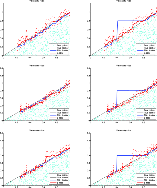
Figure 1: Resulting estimator $\tilde{\varphi}^{*}_{1}(x)$ for a uniform data set of size $n=1000$ (plus one outlier for the right panels); from top to bottom, we have the cases $\rho_{x}=2$, substituting in $\hat{\rho}_{x}$, substituting in $\tilde{\rho}_{x}$.

In Fig. 1, the estimator $\tilde{\varphi}^{*}_{1}(x)$ is first computed with the true value $\rho_{x}=2$ (top panel of the figure), then with a plug-in value of $\rho_{x}$ estimated by the Pickands estimator (middle panel) and finally with a plug-in value of $\tilde{\rho}_{x}$ estimated by the moment estimator (bottom panel). The pointwise confidence intervals are also displayed. The three right-hand panels correspond to the same data set plus one outlier. This allows us to see how our robust estimators behave in the presence of outlying points, in contrast with the FDH estimator. In particular, due to the remarkable behavior of $\tilde{\varphi}^{*}_{1}(x)$ in the Monte Carlo experiment, if we know that $\rho_{x}=2$, then we should use the top panel results and, according to our suggestion at the end of the preceding section, if $\rho_{x}$ is unknown, we should use, in this particular example, the bottom panel results, where we replace $\rho_{x}$ by its moment estimator $\tilde{\rho}_{x}$ (since here $N_{x}\leq 1000$) and continue as if $\rho_{x}$ were known. It is quite encouraging that the two panels are very similar.

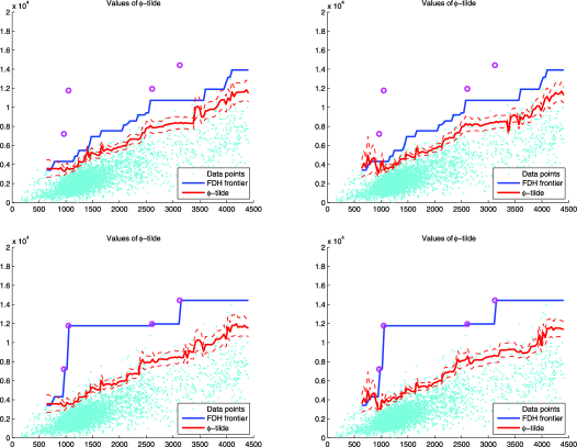
Figure 2: The resulting estimator $\tilde{\varphi}^{*}_{1}(x)$ for the French post offices. We include four extreme data points (circles) for the bottom panels. From left to right, we have the cases $\rho_{x}=2$, substituting in $\tilde{\rho}_{x}$.

3.3 An application

We use the same real data example as in [2], which undertook the frontier analysis of $9521$ French post offices observed in $1994$, with $X$ as the quantity of labor and $Y$ as the volume of delivered mail. In this illustration, we only consider the $n=4000$ observed post offices with the smallest levels $x_{i}$. We used the empirical rules explained above for selecting reasonable values for $k_{n}(x)$. The cloud of points and the resulting estimates are provided in Fig. 2.

To save space, we only represent $\tilde{\varphi}^{*}_{1}(x)$ when $\rho_{x}$ is supposed to be equal to 2 (left-hand panels) and when it is estimated by the moment estimator (right-hand panels). The FDH estimator is clearly determined by only a few very extreme points. If we delete four extreme points from the sample (represented by circles in the figure), then we obtain the pictures from the top panels: the FDH estimator changes drastically, whereas the extreme-value-based estimator $\tilde{\varphi}^{*}_{1}(x)$ is very robust to the presence of these four extreme points. We also note the considerable stability of the various forms of the estimator $\tilde{\varphi}^{*}_{1}(x)$.

4 Concluding remarks

In our approach, we provide the necessary and sufficient condition for the FDH estimator $\hat{\varphi}_{1}(x)$ to converge in distribution, we specify its asymptotic distribution with the appropriate convergence rate and provide a limit theorem for moments in a general framework. We also provide further insights and generalize the main result of [1] on robust variants of the FDH estimator, and we provide strongly consistent and asymptotically normal estimators $\hat{\rho}_{x}$ and $\tilde{\rho}_{x}$ of the unknown conditional tail index $\rho_{x}$ involved in the limit law of $\hat{\varphi}_{1}(x)$. Moreover, when the joint density of $(X,Y)$ decreases to zero or increases toward infinity at a speed of power $\beta_{x}>-1$ of the distance from the boundary, as is often assumed in the literature, we answer the question of how $\rho_{x}$ is linked to the data dimension $p+1$ and to the shape parameter $\beta_{x}$. The quantity $\beta_{x}\not=0$ describes the rate at which the density tends to infinity (in the case $\beta_{x}<0$) or to $0$ (in the case $\beta_{x}>0$) at the boundary. When $\beta_{x}=0$, the joint density is strictly positive on the frontier. We establish that $\rho_{x}=\beta_{x}+(p+1)$. As an immediate consequence, we extend the previous results of [12, 14] to the general setting where $p\geq 1$ and $\beta=\beta_{x}$ may depend on $x$.

We propose new extreme-value-based frontier estimators $\hat{\varphi}^{*}_{1}(x)$, $\tilde{\varphi}^{*}_{1}(x)$ and $\hat{\varphi}(x)$, which are asymptotically normally distributed and provide useful asymptotic confidence bands for the monotone frontier function $\varphi(x)$. These estimators have the advantage of not being limited to a bi-dimensional support and benefit from their explicit and easy formulations, which is not the case for estimators defined by optimization problems, such as local polynomial estimators (see, for example, [10]). Their asymptotic normality is derived under quite natural and general extreme value conditions, without Lipschitz conditions on the boundary and without recourse to assumptions either on the marginal distribution of $X$ or on the conditional distribution of $Y$ given $X=x$, as is often the case in both statistical and econometrics literature on frontier estimation. The study of the asymptotic properties of the different estimators considered in the present paper is easily carried out by relating them to a simple dimensionless random sample and then applying standard extreme value theory (for example, [5, 6]).

Two closely related works in boundary estimation via extreme value theory are [9], in which the estimation of the frontier function at a point $x$ is based on an increasing number of higher order statistics generated by the $Y_{i}$ observations falling into a strip around $x$, and [8], in which estimators are instead based on a fixed number of higher order statistics. The main difference with the present approach is that Hall et al. [9] only focus on estimation of the support curve of a bivariate density (that is, $p=1$) in the case $\beta_{x}>1$ (that is, the decrease in density is no more than algebraically fast), where it is known that estimators based on an increasing number of higher order statistics give optimal convergence rates. In contrast, Gijbels and Peng [8] consider the maximum of all $Y_{i}$ observations falling into a strip around $x$ and an end-point type of estimator based on three large order statistics of the $Y_{i}$’s in the strip. This methodology is closely related and comparable to our estimation method using the Pickands-type estimator, but, like the procedure of [9], it is only valid in the simple case $p=1$ and involves, in addition to the sequence $k_{n}$, an extra smoothing parameter (bandwidth of the strip) which also needs to be selected. Moreover, the asymptotic results in [8] are provided for densities of $(X,Y)$ decreasing as a power of the distance from the boundary, whereas the setup in our approach is a general one. Also, note that our transformed dimensionless data set $(Z^{x}_{1},\ldots,Z^{x}_{n})$ is constructed in such a way as to take into account the monotonicity of the frontier (the end-point of the common distribution of the $Z^{x}_{i}$’s coincides with the frontier function $\varphi(x)$), the univariate random variables $Z^{x}_{i}$ do not depend on the sample size and they allow the available results from standard extreme value theory to be easily employed, which is not the case for either of [8, 9].

It should be clear that the monotonicity constraint on the frontier is the main difference with most of the existing approaches in the statistical literature. Indeed, the joint support of a random vector $(X,Y)$ is often described in the literature as the set $\{(x,y)\mid y\leq\phi(x)\}$, where the graph of $\phi$ is interpreted as its upper boundary. As a matter of fact, the function of interest, $\varphi$, in our approach is the smallest monotone non-decreasing function which is greater than or equal to the frontier function $\phi$. To our knowledge, only the estimators FDH and DEA estimate the quantity $\varphi$. Of course, $\phi$ coincides with $\varphi$ when the boundary curve is monotone, but the construction of estimators of the end-point $\phi(x)$ of the conditional distribution of $Y$ given $X=x$ requires a smoothing procedure, which is not the case when the distribution of $Y$ is conditioned by $X\leq x$.

We illustrate how the large-sample theory applies in practice by carrying out some Monte Carlo experiments. Good estimates of $\varphi(x)$ and $\rho_{x}$ may require a large sample of the order of several thousand. Theoretically selecting the optimal extreme conditional quantiles $\hat{\varphi}_{\alpha(k_{n}(x))}$ for estimating $\varphi(x)$ and/or $\rho_{x}$ is a difficult question that is worthy of future research. Here, we suggest a simple automatic data-driven method that provides a reasonable choice of the sequence $\{k_{n}(x)\}$ for large samples.

The empirical study reveals that the simultaneous estimation of the tail index and of the frontier function requires large sample sizes to provide sensible results. The moment estimators of $\rho_{x}$ and of $\varphi(x)$ sometimes provide better estimations than the Pickands estimates and sometimes not. When considering bias and MSE, $\hat{\varphi}(x)$ and $\tilde{\rho}_{x}$ provide more accurate estimations, but when the sample size is large enough, $\hat{\varphi}^{*}_{1}(x)$ and $\hat{\rho}_{x}$ significantly improve and even seem to outperform the moment estimators. As far as the inference on $\rho_{x}$ is concerned, $\tilde{\rho}_{x}$ also provides quite reliable confidence intervals, but $\hat{\rho}_{x}$ provides more satisfactory results for sufficiently large samples. However, when inference about the frontier function itself is concerned, the moment estimator provides very poor results compared with the Pickands estimator.

On the other hand, the performance of the estimator $\tilde{\varphi}^{*}_{1}(x)$, computed when $\rho_{x}$ is known, is quite remarkable, even compared with the popular FDH. The confidence intervals for $\varphi(x)$ are very easy to compute and have quite good coverages. In addition, the results are quite stable with respect to the choice of the ‘smoothing’ parameter $k_{n}(x)$. As shown in our illustrations, the estimates also have the advantage of being robust to extreme values. This suggests, even if $\rho_{x}$ is unknown, the use of a plug-in version of $\tilde{\varphi}^{*}_{1}(x)$ for making inference on $\varphi(x)$: here, in a first step, we estimate $\rho_{x}$ (using the moment estimator, unless $N_{x}$ is large enough), then we use the asymptotic results for $\tilde{\varphi}^{*}_{1}(x)$, as if $\rho_{x}$ was known. A sensible practice is not to restrict the first step to one procedure, but rather to check that both Pickands and moment estimators point toward similar conclusions.

Appendix: Proofs

Proof of Theorem 2.1 Let $Z^{x}=Y\mathbh{1}(X\leq x)$ and $F_{x}(\cdot)=\{1-F_{X}(x)[1-F(\cdot|x)]\}\mathbh{1}(\cdot\geq 0)$. It can be easily seen that $\mathbb{P}(Z^{x}\leq y)=F_{x}(y)$ for any $y\in\mathbb{R}$. Therefore, $\{Z^{x}_{i}=Y_{i}\mathbh{1}(X_{i}\leq x)$, $i=1,\ldots,n\}$ is an i.i.d. sequence of random variables with common distribution function $F_{x}$. Moreover, it is easy to see that the right end-point of $F_{x}$ coincides with $\varphi(x)$ and that $\max_{i=1,\ldots,n}Z^{x}_{i}$ coincides with $\hat{\varphi}_{1}(x)$. Thus, assertion (i) follows from the Fisher–Tippett theorem. It is well known that the normalized maxima $b^{-1}_{n}(\hat{\varphi}_{1}(x)-\varphi(x))\stackrel{{\scriptstyle d}}{{\longrightarrow}}G$ (that is, $F_{x}$ belongs to the domain of attraction of $G=\Psi_{\rho_{x}}$) if and only if

$$\bar{F}_{x}\bigl{(}\varphi(x)-1/t\bigr{)}\in\mathit{RV}_{-\rho_{x}},$$ (8)

where $\bar{F}_{x}=1-F_{x}$. This necessary and sufficient condition is equivalent to (2). In this case, the norming constant $b_{n}$ can be taken to be equal to $\varphi(x)-\inf\{y\geq 0\mid F_{x}(y)\geq 1-\frac{1}{n}\}=\varphi(x)-\inf\{y\geq 0\mid F(y|x)\geq 1-\frac{1}{nF_{X}(x)}\}$, which gives assertion (ii). For assertion (iii), since (8) holds and $\mathbb{E}[|Z^{x}|^{k}]=F_{X}(x)\mathbb{E}(Y^{k}|X\leq x)\leq{\varphi(x)}^{k}$, it is immediate (see [16], Proposition 2.1) that $\lim_{n\rightarrow\infty}\mathbb{E}\{b^{-1}_{n}(\hat{\varphi}_{1}(x)-\varphi(x))\}^{k}=(-1)^{k}\Gamma(1+k/\rho_{x})$. Likewise, the last result follows from [16], Corollary 2.3.

Proof of Corollary 2.1 Following the proof of Theorem 2.1, we can set $b_{n}=\varphi(x)-F^{-1}_{x}(1-\frac{1}{n})$, where $F^{-1}_{x}(t)=\inf\{y\in\,]0,\varphi(x)]\mathchoice{\nobreak\,\colon}{\nobreak\,\colon}{\nobreak\,\colon\;}{\nobreak\,\colon\;}F_{x}(y)\geq t\}$ for all $t\in\,]0,1]$. It follows from (3) that $F^{-1}_{x}(t)=\varphi(x)-((1-t)/\ell_{x})^{1/\rho_{x}}$ as $t\uparrow 1$ and so $b_{n}=(1/n\ell_{x})^{1/\rho_{x}}$ for all $n$ sufficiently large.

Proof of Corollary 2.2 Under the given conditions, it can be easily seen from (3) that

$$f(x,y) = \bigl{(}\varphi(x)-y\bigr{)}^{\rho_{x}-(p+1)}$$

$${}\times\biggl{[}\ell_{x}\rho_{x}(\rho_{x}-1)\cdots(\rho_{x}-p)\frac{\partial}{\partial x^{1}}\varphi(x)\cdots\frac{\partial}{\partial x^{p}}\varphi(x)+\mathrm{o}(1)\biggr{]}\qquad\mbox{as }y\uparrow\varphi(x),$$

where the term $\mathrm{o}(1)$ depends on the partial derivatives of $x\mapsto\ell_{x}$, $x\mapsto\rho_{x}$ and $x\mapsto\varphi(x)$.

For the next proofs, we need the following lemma whose proof is quite easy and is thus omitted.

Lemma 1

Let $Z^{x}_{(1)}\leq\cdots\leq Z^{x}_{(n)}$ be the order statistics generated by the random variables $Z^{x}_{1},\ldots,Z^{x}_{n}$:

1. [(iii)]

2. If $\hat{F}_{X}(x)>0$, then $\hat{\varphi}_{1-{k}/{(n\hat{F}_{X}(x))}}(x)=Z^{x}_{(n-k)}$ for each $k\in\{0,1,\ldots,n\hat{F}_{X}(x)-1\}$.

3. For any fixed integer $k\geq 0$, we have $\hat{\varphi}_{1-{k}/{(n\hat{F}_{X}(x))}}(x)=Z^{x}_{(n-k)}$ as $n\to\infty$, with probability $1$.

4. For any sequence of integers $k_{n}\geq 0$ such that $k_{n}/n\to 0$ as $n\to\infty$, we have

   $$\hat{\varphi}_{1-{k_{n}}/{(n\hat{F}_{X}(x))}}(x)=Z^{x}_{(n-k_{n})}\qquad\mbox{as }n\to\infty,\mbox{ with probability }1.$$

Proof of Theorem 2.2 (i) Since $\varphi(x)=F^{-1}_{x}(1)$ and $\hat{\varphi}_{1}(x)=Z^{x}_{(n)}$ for all $n\geq 1$, we have $(\hat{\varphi}_{1}(x)-\varphi(x))=(Z^{x}_{(n)}-F^{-1}_{x}(1))$. Hence, if $b^{-1}_{n}(\hat{\varphi}_{1}(x)-\varphi(x))\stackrel{{\scriptstyle{d}}}{{\longrightarrow}}G_{x}$, then $b^{-1}_{n}(Z^{x}_{(n)}-F^{-1}_{x}(1))$ converges to the same distribution $G_{x}$. Therefore, following [18], Theorem 21.18, $b^{-1}_{n}(Z^{x}_{(n-k)}-F^{-1}_{x}(1))\stackrel{{\scriptstyle d}}{{\rightarrow}}H_{x}$ for any integer $k\geq 0$, where $H_{x}(y)=G_{x}(y)\sum^{k}_{i=0}(-\log G(y))^{i}/i!$. Finally, since $Z^{x}_{(n-k)}\stackrel{{\scriptstyle\mathrm{a.s.}}}{{=}}\hat{\varphi}_{1-{k}/{(n\hat{F}_{X}(x))}}(x)$ as $n\to\infty$, in view of Lemma 1(ii), we obtain $b^{-1}_{n}(\hat{\varphi}_{1-{k}/{(n\hat{F}_{X}(x))}}(x)-F^{-1}_{x}(1))\stackrel{{\scriptstyle d}}{{\longrightarrow}}H_{x}$. [

• (ii)] Writing $b^{-1}_{n}(\hat{\varphi}_{\alpha}(x)-\varphi(x))=b^{-1}_{n}(\hat{\varphi}_{\alpha}(x)-\hat{\varphi}_{1}(x))+b^{-1}_{n}(\hat{\varphi}_{1}(x)-\varphi(x))$, it suffices to find an appropriate sequence $\alpha=\alpha_{n}\rightarrow 1$ such that $b^{-1}_{n}(\hat{\varphi}_{\alpha_{n}}(x)-\hat{\varphi}_{1}(x))\stackrel{{\scriptstyle{d}}}{{\longrightarrow}}0$. Aragon et al. [1] (see equation (20)) showed that $|\hat{\varphi}_{\alpha}(x)-\hat{\varphi}_{1}(x)|\leq(1-\alpha)n\hat{F}_{X}(x)F^{-1}_{Y}(1),$ with probability $1$, for any $\alpha>0$. It thus suffices to choose $\alpha=\alpha_{n}\rightarrow 1$ such that $nb^{-1}_{n}(1-\alpha_{n})\rightarrow 0$.∎

Proof of Theorem 2.3 (i) Let $\gamma_{x}=-1/\rho_{x}$ in (8). The Pickands [15] estimate of the exponent of variation $\gamma_{x}<0$ is then given by $\hat{\gamma}_{x}:=(\log 2)^{-1}\log\{(Z^{x}_{(n-k+1)}-Z^{x}_{(n-2k+1)})/(Z^{x}_{(n-2k+1)}-Z^{x}_{(n-4k+1)})\}.$ Under (2), Condition (8) holds and so there exists $b_{n}>0$ such that $\lim_{n\to\infty}\mathbb{P}[b_{n}^{-1}(Z^{x}_{(n)}-\varphi(x))\leq y]=\Psi_{-1/\gamma_{x}}(y).$ Since this limit is unique only up to affine transformations, we have

$$\lim_{n\to\infty}\mathbb{P}\bigl{[}c_{n}^{-1}\bigl{(}Z^{x}_{(n)}-d_{n}\bigr{)}\leq y\bigr{]}=\Psi_{-1/\gamma_{x}}(-\gamma_{x}y-1)=\exp\{-(1+\gamma_{x}y)^{-1/\gamma_{x}}\}$$

for all $y\leq 0$, where $c_{n}=-\gamma_{x}b_{n}$ and $d_{n}=\varphi(x)-b_{n}$. Thus, condition (1.1) from Dekkers and de Haan [5] holds. Therefore, $\hat{\gamma}_{x}\stackrel{{\scriptstyle p}}{{\to}}\gamma_{x}$ if $k_{n}\to\infty$ and $\frac{k_{n}}{n}\to 0$, in view of [5], Theorem 2.1. This gives the weak consistency of $\hat{\rho}_{x}$ since $\hat{\gamma}_{x}\stackrel{{\scriptstyle\mathrm{a.s.}}}{{=}}-1/\hat{\rho}_{x}$ as $n\to\infty$, in view of Lemma 1(iii). [

• (ii)] Likewise, if $\frac{k_{n}}{n}\to 0$ and $\frac{k_{n}}{\log\log n}\to\infty$, then $\hat{\gamma}_{x}\stackrel{{\scriptstyle\mathrm{a.s.}}}{{\longrightarrow}}\gamma_{x}$ via [5], Theorem 2.2, and so $\hat{\rho}_{x}\stackrel{{\scriptstyle\mathrm{a.s.}}}{{\longrightarrow}}\rho_{x}$.

• We have $U(t)=\inf\{y\geq 0\mid\frac{1}{1-F_{x}(y)}\geq t\}$, which corresponds to the inverse function $(1/(1-F_{x}))^{-1}(t)$. Since $\pm t^{1-\gamma_{x}}U^{\prime}(t)\in\Pi(A)$ with $\gamma_{x}=-1/\rho_{x}<0$, it follows from [5] (see Theorem 2.3) that $\sqrt{k_{n}}(\hat{\gamma}_{x}-\gamma_{x})\stackrel{{\scriptstyle{d}}}{{\longrightarrow}}{\mathcal{N}}(0,\sigma^{2}(\gamma_{x}))$ with $\sigma^{2}(\gamma_{x})=\gamma_{x}^{2}(2^{2\gamma_{x}+1}+1)/\{2(2^{\gamma_{x}}-1)\log 2\}^{2}$ for $k_{n}\to\infty$ satisfying $k_{n}=\mathrm{o}(n/g^{-1}(n))$, where $g(t):=t^{3-2\gamma_{x}}\{U^{\prime}(t)/A(t)\}^{2}$. By using the fact that $\sqrt{k_{n}}(\hat{\rho}_{x}-\rho_{x})\stackrel{{\scriptstyle\mathrm{a.s.}}}{{=}}\sqrt{k_{n}}(-\frac{1}{\hat{\gamma}_{x}}+\frac{1}{\gamma_{x}})$ as $n\to\infty$, in view of Lemma 1(iii) and applying the delta method, we conclude that $\sqrt{k_{n}}(\hat{\rho}_{x}-\rho_{x})\stackrel{{\scriptstyle{d}}}{{\longrightarrow}}{\mathcal{N}}(0,\sigma^{2}(\rho_{x}))$ with asymptotic variance $\sigma^{2}(\rho_{x})=\sigma^{2}(\gamma_{x})/\gamma_{x}^{4}$.

• Under the regularity condition, we have $\pm\{t^{-1-{1}/{\gamma_{x}}}F_{x}^{\prime}(\varphi(x)-\frac{1}{t})-\delta F_{X}(x)\}\in\mathit{RV}_{-\kappa}$. The conclusion then follows immediately from Theorem 2.5 of [5] in conjunction with Lemma 1(iii).∎

Proof of Theorem 2.4 We have, by Lemma 1(iii), that for each $j=1,2$,

$$M^{(j)}_{n}=(1/k)\sum_{i=0}^{k-1}\bigl{(}\log Z^{x}_{(n-i)}-\log Z^{x}_{(n-k)}\bigr{)}^{j}\qquad\mbox{as }n\to\infty,\mbox{ with probability }1;$$ (9)

$-1/\tilde{\rho}_{x}$ then coincides almost surely, for all $n$ large enough, with the well-known moment estimator $\tilde{\gamma}_{x}$ (given by [6], equation (1.7)) of the index defined in (8) by $\gamma_{x}=-1/\rho_{x}$. Hence, Theorem 2.4(i) and (ii) follow from the weak and strong consistency of $\tilde{\gamma}_{x}$ proved in [6], Theorem 2.1. Likewise, Theorem 2.4(iii) follows by applying [6], Corollary 3.2, in conjunction with the delta method.

Proof of Theorem 2.5 (i) Under the regularity condition, the distribution function $F_{x}$ of $Z^{x}$ has a positive derivative $F_{x}^{\prime}(y)=F_{X}(x)F^{\prime}(y|x)$ for all $y>0$ such that $F^{\prime}_{x}(\varphi(x)-\frac{1}{t})\in\mathit{RV}_{1+{1}/{\gamma_{x}}}$. Therefore, according to [5] (see Theorem 3.1),

$$\sqrt{2k_{n}}\frac{Z^{x}_{(n-k_{n}+1)}-F_{x}^{-1}(1-p_{n})}{Z^{x}_{(n-k_{n}+1)}-Z^{x}_{(n-2k_{n}+1)}}$$

is asymptotically normal with mean zero and variance $2^{2\gamma_{x}+1}\gamma_{x}^{2}/(2^{\gamma_{x}}-1)^{2}$. We conclude by using the facts that $F_{x}^{-1}(1-p_{n})=\varphi_{1-{p_{n}}/{F_{X}(x)}}(x)$ and

$$\sqrt{2k_{n}}\frac{Z^{x}_{(n-k_{n}+1)}-F_{x}^{-1}(1-p_{n})}{Z^{x}_{(n-k_{n}+1)}-Z^{x}_{(n-2k_{n}+1)}}$$

$$\quad\stackrel{{\scriptstyle\mathrm{a.s.}}}{{=}}\sqrt{2k_{n}}\frac{\hat{\varphi}_{1-{(k_{n}-1)}/{(n\hat{F}_{X}(x))}}(x)-F_{x}^{-1}(1-p_{n})}{\hat{\varphi}_{1-{(k_{n}-1)}/{(n\hat{F}_{X}(x))}}(x)-\hat{\varphi}_{1-{(2k_{n}-1)}/{(n\hat{F}_{X}(x))}}(x)}\qquad\mbox{as }n\to\infty.$$

[

• (ii)] We have $\hat{\varphi}^{*}_{1}(x)\stackrel{{\scriptstyle\mathrm{a.s.}}}{{=}}\frac{Z^{x}_{(n-k_{n}+1)}-Z^{x}_{(n-2k_{n}+1)}}{2^{-\hat{\gamma}_{x}}-1}+Z^{x}_{(n-k_{n}+1)}$ as $n\to\infty$. Following [5], Theorem 3.2,

  $$\frac{\sqrt{2k_{n}}(\hat{\varphi}^{*}_{1}(x)-\varphi(x))}{Z^{x}_{(n-k_{n}+1)}-Z^{x}_{(n-2k_{n}+1)}}$$

  is then asymptotically normal with mean zero and variance $3\gamma_{x}^{2}2^{2\gamma_{x}-1}/(2^{\gamma_{x}}-1)^{6}$.

• Let $E_{(1)}\leq\cdots\leq E_{(n)}$ be the order statistics of i.i.d. exponential variables $E_{1},\ldots,E_{n}$. Then, $\{Z^{x}_{(n-k+1)}\}_{k=1}^{n}\stackrel{{\scriptstyle{d}}}{{=}}\{U(\mathrm{e}^{E_{(n-k+1)}})\}_{k=1}^{n}$. Writing $V(t):=U(\mathrm{e}^{t})$, we obtain

  $$\sqrt{2k_{n}}\biggl{\{}\frac{1}{2^{-\gamma_{x}}-1}+\frac{Z^{x}_{(n-k_{n}+1)}-\varphi(x)}{Z^{x}_{(n-k_{n}+1)}-Z^{x}_{(n-2k_{n}+1)}}\biggr{\}}$$

  $$\quad\stackrel{{\scriptstyle{d}}}{{=}}\sqrt{2k_{n}}\biggl{\{}\frac{1}{2^{-\gamma_{x}}-1}+\frac{V(E_{(n-k_{n}+1)})-\varphi(x)}{V(E_{(n-k_{n}+1)})-V(E_{(n-2k_{n}+1)})}\biggr{\}}$$

  $$\quad=\biggl{[}-\sqrt{2k_{n}}\biggl{\{}\frac{V(\infty)-V(\log{n}/{(2k_{n})})}{V^{\prime}(\log{n}/{(2k_{n})})}+\frac{1}{\gamma_{x}}\biggr{\}}$$

  $$\qquad\hskip 4.0pt{}+\sqrt{2k_{n}}\biggl{\{}\frac{V(E_{(n-k_{n}+1)})-V(E_{(n-2k_{n}+1)})}{2^{\gamma_{x}}V^{\prime}(E_{(n-2k_{n}+1)})}-\frac{1-2^{-\gamma_{x}}}{\gamma_{x}}\biggr{\}}\frac{2^{\gamma_{x}}}{1-2^{\gamma_{x}}}\frac{V^{\prime}(E_{(n-2k_{n}+1)})}{V^{\prime}(\log{n}/{(2k_{n})})}$$

  $$\hskip 4.0pt\qquad{}-\frac{\sqrt{2k_{n}}}{\gamma_{x}}\biggl{\{}\frac{V^{\prime}(E_{(n-2k_{n}+1)})}{V^{\prime}(\log{n}/{(2k_{n})})}-1-\gamma_{x}\frac{V(E_{(n-k_{n}+1)})-V(\log{n}/{(2k_{n})})}{V^{\prime}(\log{n}/{(2k_{n})})}\biggr{\}}\biggr{]}$$

  $$\hskip 33.0pt{}\times\frac{V^{\prime}(\log{n}/{(2k_{n})})}{V(E_{(n-k_{n}+1)})-V(E_{(n-2k_{n}+1)})}.$$

  The first term on the right-hand side tends to zero as established by Dekkers and de Haan ([5], Proof of Theorem 3.2). The second term converges in distribution to ${\mathcal{N}}(0,1)\times\frac{2^{\gamma_{x}}}{1-2^{\gamma_{x}}}$, in view of Lemma 3.1 and [5], Corollary 3.1. The third term converges in probability to $\frac{\gamma_{x}}{2^{\gamma_{x}}-1}$ by the same Corollary 3.1. This ends the proof of (iii), in conjunction with the fact that

  $$\sqrt{2k_{n}}\frac{\tilde{\varphi}^{*}_{1}(x)-\varphi(x)}{\hat{\varphi}_{1-{(k_{n}-1)}/{(n\hat{F}_{X}(x))}}(x)-\hat{\varphi}_{1-{(2k_{n}-1)}/{(n\hat{F}_{X}(x))}}(x)}$$

  $$\quad=\sqrt{2k_{n}}\biggl{\{}\frac{1}{2^{-\gamma_{x}}-1}+\frac{Z^{x}_{(n-k_{n}+1)}-\varphi(x)}{Z^{x}_{(n-k_{n}+1)}-Z^{x}_{(n-2k_{n}+1)}}\biggr{\}}\qquad\mbox{as }n\to\infty,$$

  with probability $1$.∎

Proof of Theorem 2.6 Write $\bar{F}_{x}(y):=F_{X}(x)[1-F(y|x)]$ and $F_{x}(y):=1-\bar{F}_{x}(y)$ for all $y\geq 0$. Let $R_{x}(y):=-\log\{\bar{F}_{x}(y)\}$ for all $y\in[0,\varphi(x)[$ and let $E_{(n-k_{n}+1)}$ be the statistic of order $n-k_{n}+1$ generated by $n$ independent standard exponential random variables. $Z^{x}_{(n-k_{n}+1)}$ then has the same distribution as $R^{-1}_{x}[E_{(n-k_{n}+1)}]$, where $R^{-1}_{x}(t):=\inf\{y\geq 0\mid R_{x}(y)\geq t\}=\inf\{y\geq 0\mid F_{x}(y)\geq 1-\mathrm{e}^{-t}\}:=F_{x}^{-1}(1-\mathrm{e}^{-t}).$ Hence,

$$Z^{x}_{(n-k_{n}+1)}-F_{x}^{-1}\biggl{(}1-\frac{k_{n}}{n}\biggr{)}$$

$$\quad\stackrel{{\scriptstyle d}}{{=}}R^{-1}_{x}\bigl{[}E_{(n-k_{n}+1)}\bigr{]}-R^{-1}_{x}\biggl{[}\log\biggl{(}\frac{n}{k_{n}}\biggr{)}\biggr{]}$$

$$\quad=\biggl{[}E_{(n-k_{n}+1)}-\log\biggl{(}\frac{n}{k_{n}}\biggr{)}\biggr{]}(R^{-1}_{x})^{\prime}\biggl{[}\log\biggl{(}\frac{n}{k_{n}}\biggr{)}\biggr{]}$$

$$\qquad{}+\frac{1}{2}\biggl{[}E_{(n-k_{n}+1)}-\log\biggl{(}\frac{n}{k_{n}}\biggr{)}\biggr{]}^{2}(R^{-1}_{x})^{\prime\prime}[\delta_{n}],$$

provided that $E_{(n-k_{n}+1)}\wedge\log(n/k_{n})<\delta_{n}<E_{(n-k_{n}+1)}\vee\log(n/k_{n})$. By the regularity condition (3), we have that $R^{-1}_{x}(t)=\varphi(x)-(\mathrm{e}^{-t}/\ell_{x})^{1/\gamma_{x}}$ for all $t$ large enough. Therefore, for all $n$ sufficiently large,

$$\{\rho_{x}k^{1/2}_{n}/(k_{n}/n\ell_{x})^{1/\rho_{x}}\}\bigl{[}Z^{x}_{(n-k_{n}+1)}-F^{-1}_{x}(1-k_{n}/n)\bigr{]}$$

$$\quad\stackrel{{\scriptstyle d}}{{=}}k^{1/2}_{n}\bigl{[}E_{(n-k_{n}+1)}-\log(n/k_{n})\bigr{]}$$

$$\qquad{}-\{k^{1/2}_{n}/2\rho_{x}\}\bigl{[}E_{(n-k_{n}+1)}-\log(n/k_{n})\bigr{]}^{2}\exp\{-[\delta_{n}-\log(n/k_{n})]/\rho_{x}\}.$$

Since $k^{1/2}_{n}[E_{(n-k_{n}+1)}-\log(n/k_{n})]\stackrel{{\scriptstyle{d}}}{{\rightarrow}}\mathcal{N}(0,1)$ and $|\delta_{n}-\log(n/k_{n})|\leq|E_{(n-k_{n}+1)}-\break\log(n/k_{n})|\stackrel{{\scriptstyle p}}{{\rightarrow}}0$ as $n\rightarrow\infty$, we obtain $\{\rho_{x}k^{1/2}_{n}/(k_{n}/n\ell_{x})^{1/\rho_{x}}\}[Z^{x}_{(n-k_{n}+1)}-F^{-1}_{x}(1-k_{n}/n)]\stackrel{{\scriptstyle{d}}}{{\longrightarrow}}\mathcal{N}(0,1)$ as $n\rightarrow\infty$. Since $F^{-1}_{x}(t)=\varphi(x)-((1-t)/\ell_{x})^{1/\rho_{x}}$ for all $t<1$ large enough, we have $\varphi(x)-F^{-1}_{x}(1-\frac{k_{n}}{n})=(k_{n}/n\ell_{x})^{1/\rho_{x}}$ for all $n$ sufficiently large. Thus, $\{\rho_{x}k^{1/2}_{n}/(k_{n}/n\ell_{x})^{1/\rho_{x}}\}\times[Z^{x}_{(n-k_{n}+1)}+(k_{n}/n\ell_{x})^{1/\rho_{x}}-\varphi(x)]\stackrel{{\scriptstyle{d}}}{{\to}}\mathcal{N}(0,1)$ as $n\to\infty$. We conclude by using the fact that $Z^{x}_{(n-k_{n}+1)}\stackrel{{\scriptstyle\mathrm{a.s.}}}{{=}}\hat{\varphi}_{1-{(k_{n}-1)}/{(n\hat{F}_{X}(x))}}(x)$ as $n\to\infty$.

Proof of Theorem 2.7 (i) As shown in the proof of Theorem 2.5(i), we have $F^{\prime}_{x}(\varphi(x)-\frac{1}{t})\in\mathit{RV}_{1+1/\gamma_{x}}$. Then, by applying Dekkers et al. [6], Theorem 5.1, in conjunction with (9), we get

$$\sqrt{k_{n}}\bigl{\{}Z^{x}_{(n-k_{n})}-F^{-1}_{x}(1-p_{n})\bigr{\}}/M^{(1)}_{n}Z^{x}_{(n-k_{n})}\stackrel{{\scriptstyle{d}}}{{\longrightarrow}}{\mathcal{N}}\bigl{(}0,V_{4}(-1/\gamma_{x})\bigr{)}.$$

The proof is completed by simply using the fact that $F^{-1}_{x}(1-p_{n})=\varphi_{1-{p_{n}}/{(F_{X}(x))}}(x)$ and $Z^{x}_{(n-k_{n})}\stackrel{{\scriptstyle\mathrm{a.s.}}}{{=}}\hat{\varphi}_{1-{k_{n}}/{(n\hat{F}_{X}(x))}}(x)$ as $n\to\infty$. [

• (ii)] Since $Z^{x}_{(n-k_{n})}\stackrel{{\scriptstyle\mathrm{a.s.}}}{{=}}\hat{\varphi}_{1-{k_{n}}/{(n\hat{F}_{X}(x))}}(x)$ and $\tilde{\gamma}_{x}\stackrel{{\scriptstyle\mathrm{a.s.}}}{{=}}-1/\tilde{\rho}_{x}$ as $n\to\infty$, we have $\hat{\varphi}(x)\stackrel{{\scriptstyle\mathrm{a.s.}}}{{=}}Z^{x}_{(n-k_{n})}M^{(1)}_{n}(1-1/\tilde{\gamma}_{x})+Z^{x}_{(n-k_{n})}$ as $n\to\infty$. It is then easy to see from (9) that $\hat{\varphi}(x)$ coincides almost surely, for all $n$ large enough, with the end-point estimator $\hat{x}^{*}_{n}$ of $F^{-1}_{x}(1)$ introduced by [6], equation (4.8). It is also easy to check that $U(t)=(1/(1-F_{x}))^{-1}(t)$ satisfies the conditions of [6], Theorem 3.1, with $\gamma_{x}=-1/\rho_{x}<0$. According to [6], Theorem 5.2, we then have $\sqrt{k_{n}}\{\hat{x}^{*}_{n}-F^{-1}_{x}(1)\}/M^{(1)}_{n}Z^{x}_{(n-k_{n})}(1-\tilde{\gamma}_{x})\stackrel{{\scriptstyle{d}}}{{\longrightarrow}}{\mathcal{N}}(0,V_{5}(-1/\gamma_{x})),$ which gives the desired convergence in distribution of Theorem 2.7(ii) since $F^{-1}_{x}(1)=\varphi(x)$, $\hat{x}^{*}_{n}\stackrel{{\scriptstyle\mathrm{a.s.}}}{{=}}\hat{\varphi}(x)$, $\tilde{\gamma}_{x}\stackrel{{\scriptstyle\mathrm{a.s.}}}{{=}}-1/\tilde{\rho}_{x}$ and $Z^{x}_{(n-k_{n})}\stackrel{{\scriptstyle\mathrm{a.s.}}}{{=}}\hat{\varphi}_{1-{k_{n}}/{(n\hat{F}_{X}(x))}}(x)$ as $n\to\infty$.∎

References

• [1] Aragon, Y., Daouia, A. and Thomas-Agnan, C. (2005). Nonparametric frontier estimation: A conditional quantile-based approach. Econometric Theory 21 358–389. MR2179542
• [2] Cazals, C., Florens, J.P. and Simar, L. (2002). Nonparametric frontier estimation: A robust approach. J. Econometrics 106 1–25. MR1875525
• [3] Daouia, A. and Ruiz-Gazen, A. (2006). Robust nonparametric frontier estimators: Influence function and qualitative robustness. Statist. Sinica 16 1233–1253. MR2327488
• [4] Daraio, C. and Simar, L. (2007). Advanced Robust and Nonparametric Methods in Efficiency Analysis: Methodology and Applications. New York: Springer.
• [5] Dekkers, A.L.M. and de Haan, L. (1989). On the estimation of extreme-value index and large quantiles estimation. Ann. Statist. 17 1795–1832. MR1026314
• [6] Dekkers, A.L.M., Einmahl, J.H.J. and de Haan, L. (1989). A moment estimator for the index of an extreme-value distribution. Ann. Statist. 17 1833–1855. MR1026315
• [7] Deprins, D., Simar, L. and Tulkens, H. (1984). Measuring labor inefficiency in post offices. In The Performance of Public Enterprises: Concepts and Measurements (M. Marchand, P. Pestieau and H. Tulkens, eds.) 243–267. Amsterdam: North-Holland.
• [8] Gijbels, I. and Peng, L. (2000). Estimation of a support curve via order statistics. Extremes 3 251–277. MR1856200
• [9] Hall, P., Nussbaum, M. and Stern, S.E. (1997). On the estimation of a support curve of indeterminate sharpness. J. Multivariate Anal. 62 204–232. MR1473874
• [10] Hall, P., Park, B.U. and Stern, S.E. (1998). On polynomial estimators of frontiers and boundaries. J. Multivariate Anal. 66 71–98. MR1648521
• [11] Hardle, W., Park, B.U. and Tsybakov, A.B. (1995). Estimation of non-sharp support boundaries. J. Multivariate Anal. 43 205–218. MR1370400
• [12] Hwang, J.H., Park, B.U. and Ryu, W. (2002). Limit theorems for boundary function estimators. Statist. Probab. Lett. 59 353–360. MR1935669
• [13] Korostelev, A., Simar, L. and Tsybakov, A.B. (1995). Efficient estimation of monotone boundaries. Ann. Statist. 23 476-489. MR1332577
• [14] Park, B., Simar, L. and Weiner, C. (2000). The FDH estimator for productivity efficiency scores: Asymptotic properties. Econometric Theory 16 855–877. MR1803713
• [15] Pickands, J. (1975). Statistical inference using extreme order statistics. Ann. Statist. 3 119–131. MR0423667
• [16] Resnick, S.I. (1987). Extreme Values, Regular Variation, and Point Processes. New York: Springer. MR0900810
• [17] Resnick, S.I. (2007). Heavy-Tail Phenomena: Probabilistic and Statistical Modeling. New York: Springer. MR2271424
• [18] van der Vaart, A.W. (1998). Asymptotic Statistics. Cambridge Series in Statistical and Probabilistic Mathematics 3. Cambridge: Cambridge Univ. Press. MR1652247