Induced soliton ejection from a continuous-wave source waveguided by an optical pulse-soliton train

Abstract

It has been established for some time that high-power pump can trap a probe beam of lower intensity that is simultaneously propagating in a Kerr-type optical medium, inducing a focusing of the probe with the emergence of modes displaying solitonic properties. To understand the mechanism by which such self-sustained modes are generated, and mainly the changes on probe spectrum induced by the cross-phase-modulation effect for an harmonic probe trapped by a multiplex of temporal pulses, a linear equation (for the probe) and a nonlinear Schrödinger equation (for the pump) both coupled by a cross-phase-modulation term, are considered simultaneously. In general the set of coupled probe-pump equations is not exactly tractable at any arbitrary value of the ratio of the cross-phase to the self-phase modulation strengths. However, for certain values of this ratio, the probe modulation wavector develops into $|n,l\textgreater$ quantum states involving $2n+1$ soliton-shaped eigenfunctions which spectral properties can be characterized unambiguously. Solutions of the probe equation give evidence that the competition between the self-phase and cross-phase modulations leads to a broadband spectrum, with the possibility of a quasi-continuum of soliton modes when the cross-phase-modulation coupling is strong enough.

1 Introduction

In two classic papers [1, 2], by solving the master-slave optical system

$$-i\frac{\partial A_{1}}{\partial z}-\frac{1}{2k_{1}}\frac{\partial^{2}A_{1}}{\partial x^{2}} = \frac{n_{2}^{spm}k_{1}}{n_{0}}|A_{1}|^{2}A_{1},$$ (1)

$$-i\frac{\partial A_{2}}{\partial z}-\frac{1}{2k_{2}}\frac{\partial^{2}A_{2}}{\partial x^{2}} = \frac{n_{2}^{ipm}k_{2}}{n_{0}}|A_{1}|^{2}A_{2},$$ (2)

the author predicted that ultrafast pulses with energies lower than that required to self-sustain soliton shape in the anomalous dispersion regime of an optical medium may preserve their shape, provided an intense copropagating pump of a different color (i.e. wavelength) and a longer duration typical of soliton is present. Since this key input as well as the subsequent experimental evidences reported in [3, 4] it has become evident that besides their most common applications in long-distance transmission of high-power signals [5, 6], solitons could be prime candidates for controlling light by light [7, 8]. More advanced studies have been carried out in recent years based on numerical simulations, and revealed that due to their unique stability properties solitons provide excellent and reliable guiding structures for reconfigurable low-power signals and re-routinable high-power pulses [9, 10]. Particularly attracting is the possibility to construct soliton networks that can be used as nonlinear waveguide arrays, as established in the landscape of recent experiments [11, 12, 13, 14, 15, 16] emphasizing the outstanding robustness of the periodic lattices of optical solitons with flexible (hence controllable) refractive index modulation depth and period that are induced all-optically. In general, these periodic optical-soliton structures form in continuous nonlinear media where they develop into optically imprinted modulations with some effective refractive index. Given the tunable character of the effective refractive index as well as the flexible modulation period, a great number of new opportunities for all-optical manipulation of light can be envisaged since in this case, periodic optical-soliton waveguides can operate in both weak and strong-coupling regimes depending on the depth of refractive index modulation. Transmission techniques exploiting optically-induced waveguiding configurations with solitons are now common in several communication media such as laser [17], photon [9, 10, 18] systems and photorefractive semiconductor [19] media.
The present work aims at extending the phenomenon of signal reconfiguration by strong optical fields to the context of an harmonic cw beam trapped in the guiding structure of a periodic pulse train. As in a previous study [18] we assume that due to the competition between the self-phase modulation (SPM) and cross-phase modulation (XPM) [17, 20, 21, 22, 23] effects, the low-power probe can be reshaped giving rise to self-sustained optical signals trapped within the guiding structure of the temporal pulse multiplex. But before it is relavant to stress that the groundstate spectrum of the trapped probe in the case of one-soliton pump has been discussed in details [9, 10]. Thus, it is established both analytically and numerically that even in the steady-state regime of the pump propagation the probe groundstate is not well defined at any arbitrary value of the ratio between the cross-phase and self-phase modulation strengths but only for some specific choices of this ratio. For one particular value of this ratio involving well defined optical structures, it has been found [1, 2, 9] that the fundamental mode of the trapped probe groundstate consists of a single-pulse soliton with finite momentum. Very recently, considering the same particular value of the XPM to the SPM ratio we pointed out [18] that the physics of the pump-probe system turns to be quite rich if the pump is a periodic train of pulses, time-multiplexed at the input of an optical medium as for instance an optical fiber prior to propagation. Namely, we found that in response to this temporal pulse multiplexing in the pump the trapped probe spectrum could burst into a band reflecting distinct possible induced fundamental soliton modes.
Still the competition between the SPM and XPM effects is never of the same order and can change from one optical medium to another, implying quite distinct features and properties of the probe groundstate. In this last respect, for the value of the XPM to the SPM ratio considered in our previous study we found [18] three distinct soliton modes, and observed that they form a complete orthogonal set of $|n,l\textgreater$ eigenstates two of which were almost degenerate.
In the present study we shall go beyond previous considerations in terms of the order of the competition between the XPM and SPM effects [9, 10, 18], by considering two new representative but larger values of the ratio of their strengths. Our ultimate goal through such assumptions is to point out an increasingly broadband and highly degenerate spectrum for the induced-soliton states in the probe, so broad and degenerate that the probe field can develop into a soliton quasi-continuum for sufficiently strong XPM effect relative to the SPM effect.

2 Probe source spectral problem

The pump-probe system of our current interest is described by the two coupled equations [1, 2, 9, 18]:

$$i\frac{\partial A_{1}}{\partial z} + \frac{1}{2}\frac{\partial^{2}A_{1}}{\partial t^{2}}+\xi|A_{1}|^{2}\,A_{1}=0,$$ (3)

$$i\frac{\partial A_{2}}{\partial z} + \frac{1}{2}D\frac{\partial^{2}A_{2}}{\partial t^{2}}+i\lambda\frac{\partial A_{2}}{\partial t}+\beta|A_{1}|^{2}\,A_{2}=0,$$ (4)

where (3) is the pump equation assumed to describe propagation in a Kerr-type optical fiber in the anomalous dispersion regime [1, 2], and (4) is the linear equation corresponding to the harmonic probe. The quantities $A_{1}$ and $A_{2}$ are envelopes of the pump and probe respectively, $D$ is the group-velocity dispersion of the probe (here taken arbitrary to account for possible difference with that of the pump), $\xi$ is the SPM coefficient generic of nonlinearity in the pump source, $\lambda$ in the second equation is the (temporal) walk-off between the pump and probe while $\beta$ measures the strength of the cross-phase interaction between the pump and probe.
Our main point of focus is the probe equation (4) which, as it stands, requires an explicit knowledge of shape profile of the fundamental mode composing the pump signal. As we are interested in a pump consisting of a train of time-multiplexed pulses, we focus on a classic implementation where the separation between pulses in the soliton train is varied by controlling their mutual interactions, namely via the dispersion-management technique (see more detailed discussions e.g. in [24, 25, 26]). It is known that such a periodic structure of equally separated pulses can well be represented by the sum:

$$|A_{1}(z_{0},t)|=\sum_{n=1}^{N}{|Q_{n}|\,sech\,Q_{n}\left(t-t_{n}-\omega_{n}z_{0}\right)}$$ (5)

where, following parameter definitions in [25], the quantity $N$ represents the number of channels in the time domain, $t_{n}$ is the initial temporal position of a given $n^{th}$ pulse in the input multiplex while $Q_{n}$ and $\omega_{n}$ are the associate amplitude and central frequency respectively. The input time-multiplexed pulse structure (5) can be reduced to the following single-valued function, using the exact summation rule for $sech$ functions [27, 28]:

$$A_{1}(z,t)=\frac{Q}{\sqrt{\xi}}\,dn\left[Q\left(t-t_{0}-\omega z\right),\kappa\right]e^{i\left[\omega t+\frac{\kappa^{2}\omega^{2}}{2}z+\frac{Q^{2}-2\omega^{2}}{2}z\right]},$$ (6)

which quite remarkably, coincides with the exact periodic-soliton solution of the pump equation (3) [29, 30]. It is instructive specifying that $dn$ in the above formula is the Jacobi elliptic function of modulus $\kappa$, $Q$ is the amplitude and $\omega$ is the characteristic pulse frequency. The Jacobi elliptic function $dn$ is periodic in its arguments $(z,t)$ and for the solution (6), the temporal period is $\tau_{0}=2K(\kappa)/Q$ where $K(\kappa)$ is the elliptic integral of the first kind. In optical communication such solution has been claimed [29, 30]) to represents a steady-state structure describing a train of pulses, which equal temporal separation coincides with the period $\tau_{0}$ of the $dn$ function. It is useful to end the current discussion on properties of the $dn$ function by remarking that the one-to-one correspondance between (6) and the piecewise multi-soliton signal intensity defined in (6), can easily be established by setting $t_{n}=t_{0}+n\tau_{0}$ with $t_{0}$ an initial position, and constraining all pulses to have common amplitude $Q_{n}$ (hence common central frequency width $\omega_{0}=\omega$).
Now turning to the probe equation (4) we remark to start that since the nonlinearity here proceeds from the XPM coupling to the pump, it is ready to anticipate arguing that any nonlinear mode emerging in the probe should be induced by the pump signal. Therefore, to ensure full account of the steady-state feature of the pump soliton as well as the temporal multiplexing at the fiber entry, we must also express the envelope of the probe as a steady wave i.e.:

$$A_{2}(z,t)=u(t)\,e^{i\left[kz+\phi(t)\right]},$$ (7)

where $u(t)$ is the temporal core of the probe envelope which is actually trapped by the pump, $k$ is the wavector for the probe modulation in the pump trap while $\phi(t)$ is a momentum-independent temporal phase shift. Inserting (7) in (4) and taking $D>0$ we obtain:

$$-\frac{\partial^{2}u}{\partial\tau^{2}}+\left[\frac{\beta}{\xi d}\kappa^{2}sn^{2}(\tau)-h(k)\right]u=0,\hskip 8.5359pt\phi_{t}=-\frac{\lambda}{d},$$ (8)

$$\tau=Q(t-t_{0}),\hskip 8.5359pth(k)=\frac{2\beta}{\xi d}+\frac{2\epsilon}{Q^{2}d},\hskip 8.5359pt\epsilon=k+\frac{\lambda^{2}}{2d}.$$ (9)

Now setting

$$n(n+1)=\frac{2\beta}{\xi D},$$ (10)

equation (8) becomes:

$$u_{\tau\tau}+\left[h(k)-n(n+1)\kappa^{2}sn^{2}(\tau)\right]u=0.$$ (11)

When $\kappa=1$, equation (11) reduces exactly to the Associated Legendre equation studied in refs. [1, 2, 9, 10] in the context of a single-soliton pump interacting with an harmonic probe. In the next section, we investigate spectral properties of the eigenvalue equation (11) for values of $\beta/\xi D$ larger than those considered so far, in particualr for orders of the competition between the XPM and SPM effects higher than the lowest order discussed in [18].

3 Spectral properties of $|n(=2,3),\,l\textgreater$ soliton eigenstates

3.1 The $|2,l\textgreater$ soliton modes

When $\beta=3\,\xi D$, formula (10) yields $n=2$ and the spectral problem for the probe in the pump trap takes the explicit form:

$$u_{\tau\tau}+\left[h(k)-6\kappa^{2}sn^{2}(\tau)\right]u=0.$$ (12)

Equation (12), which is member of the so-called Lamé eigenvalue problem [31, 32], is known to admit both extended-wave and localized-wave solutions. For the problem under consideration localized-wave solutions are best appropriate for they represent probe structures that involve low-momentum exchanges with the pump signal. Moreover, their localized shapes are key asset in our quest for stable long-standing signals with soliton features. In the specific case of equation (12) there are exactly five distinct localized modes that are induced by the soliton trap in the probe groundstate. These five modes, which can be induced simultaneously in the probe for a pump of sufficiently high intensity, form a complete set and the associate spectrum consists of the following eigenstates listed from the lowest to the highest modes (in terms of the magntitudes of their respective modulation wavectors $k_{l}$) [31, 32]:
$|2,1\textgreater$ soliton mode:

$$u_{1}(\tau) = u_{1,0}(\kappa)\,cn\left(\tau-\tau_{0}\right)\,sn\left(\tau-\tau_{0}\right),$$

$$k_{1}(\kappa) = k_{\lambda}+Q^{2}D\,(2-\kappa^{2})/2,$$ (13)

$|2,2\textgreater$ soliton mode:

$$u_{2}(\tau) = u_{2,0}(\kappa)\,\left[sn^{2}\left(\tau-\tau_{0}\right)-\frac{1+\kappa^{2}-\sqrt{1-\kappa^{2}(1-\kappa^{2})}}{3\kappa^{2}}\right],$$

$$k_{2}(\kappa) = k_{\lambda}+\frac{Q^{2}D}{2}\,\left[2(2-\kappa^{2})-\sqrt{1-\kappa^{2}(1-\kappa^{2})}\right],$$ (14)

$|2,3\textgreater$ soliton mode:

$$u_{3}(\tau) = u_{3,0}(\kappa)\,\left[sn^{2}\left(\tau-\tau_{0}\right)-\frac{1+\kappa^{2}+\sqrt{1-\kappa^{2}(1-\kappa^{2})}}{3\kappa^{2}}\right],$$

$$k_{3}(\kappa) = k_{\lambda}+\frac{Q^{2}D}{2}\,\left[2(2-\kappa^{2})+\sqrt{1-\kappa^{2}(1-\kappa^{2})}\right],$$ (15)

$|2,4\textgreater$ soliton mode:

$$u_{4}(\tau) = u_{4,0}(\kappa)\,dn\left(\tau-\tau_{0}\right)\,sn\left(\tau-\tau_{0}\right),$$

$$k_{4}(\kappa) = k_{\lambda}+Q^{2}D\,(5-4\kappa^{2})/2,$$ (16)

$|2,5\textgreater$ soliton mode:

$$u_{5}(\tau) = u_{5,0}(\kappa)\,cn\left(\tau-\tau_{0}\right)\,dn\left(\tau-\tau_{0}\right),$$

$$k_{5}(\kappa) = k_{\lambda}+Q^{2}D\,(5-\kappa^{2})/2.$$ (17)

In the above formula $cn$ and $sn$ are Jacobi elliptic functions while $k_{\lambda}=\lambda^{2}/2D$ is a wavector shift associate with the temporal walk-off $\lambda$. According to expressions of the characteristic wavectors of the five soliton modes, this wavector shift is uniform and constant so that the temporal walk-off is not relevant to the generation mechanism of the localized modes, but strictly the competition between the XPM and SPM couplings.
In figure 1, we sketched profiles of the intensities $|u(\tau)|$ of the five soliton modes obtained above for arbitrary values of their normalization amplitudes. The left graphs are intensity profiles of the induced-soliton signals for $\kappa=0.95$, while the right graphs represent same quantities for $\kappa=1$.

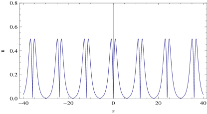
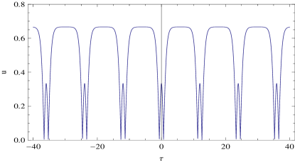
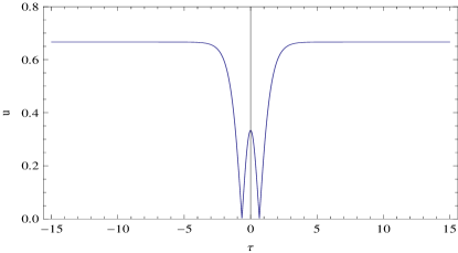
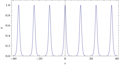
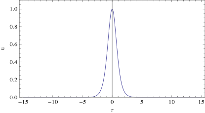
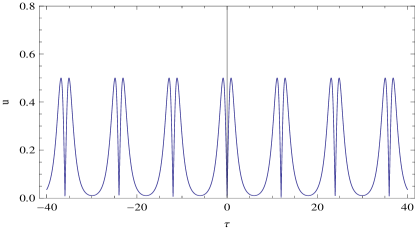
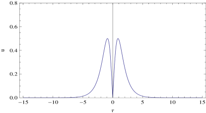
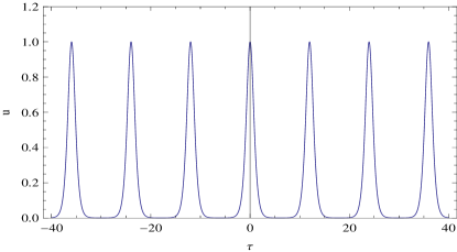
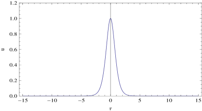
Figure 1: Intensities $|u(\tau)|$ of the five soliton modes $|2,l\textgreater$ given by (13)-(17), for $\kappa=0.95$ (left graphs) and $\kappa=1$ (right graphs). Modes are displayed from the lowest (top graph) to the highest (bottom graph) soliton eigenstates in terms of their modulation wavectors.

According to the left graphs of figure 1, the five localized modes have periodic-wavetrain features similar to the pump structure when $0\leq\kappa<1$. Moreover, as in this last structure where the fundamental signal is pulse shaped, the five modes are pulse-core periodic signals though with distinct periodicities. Indeed, the first (i.e. lowest) and fourth modes are period-one double-pulse soliton trains, the second is a period-two one-pulse soliton train whereas the third and fifth modes are period-one one-pulse soliton trains. Shapes of the fundamental solitons characterizing the five soliton modes are displayed in the right graphs of figure 1, they are consistent both with the general analytical expressions (13)-(17) when plotted for $\kappa=1$, and with the following explicit formula obtained from these solutions in the limit $\kappa\rightarrow 1$:

$$u_{1}(\tau) \propto sech\left(\tau-\tau_{0}\right)\,tanh\left(\tau-\tau_{0}\right),$$

$$k_{1} = k_{\lambda}+Q^{2}D/2,$$ (18)

$$u_{2}(\tau) \propto \left[\frac{2}{3}-sech^{2}\left(\tau-\tau_{0}\right)\right],$$

$$k_{2} = k_{\lambda}+Q^{2}D/2,$$ (19)

$$u_{3}(\tau) \propto -sech^{2}\left(\tau-\tau_{0}\right),$$

$$k_{3} = k_{\lambda}+3Q^{2}D/2,$$ (20)

$$u_{4}(\tau) \propto sech\left(\tau-\tau_{0}\right)\,tanh\left(\tau-\tau_{0}\right),$$

$$k_{4} = k_{\lambda}+Q^{2}D/2,$$ (21)

$$u_{5}(\tau) \propto sech^{2}\left(\tau-\tau_{0}\right),$$

$$k_{5} = k_{\lambda}+2Q^{2}D.$$ (22)

To give a complete description of spectral properties of the $|2,l\textgreater$ probe soliton modes, we also plotted the variations of their modulation wavectors with the paramater $\kappa$. In effect, the modulus $\kappa$ of Jacobi elliptic functions emerged above as governing the stability of wavetrain structures of both the pump and the induced probe solitons, as well as their decay toward characteristic fundamental soliton modes. Since modes are characterized by their modulation wavectors within the pump trap and given that the modulation wavector determines the amount of energy cost to the pump for mode formation and stable, we expect the variations of the different $k_{l=1,...,5}$ obtained above to provide relevant additional insight onto spectral properties of the five modes.
Figure (2) displays the wavector spectrum incompassing the five probe modes (13)-(17), where wavectors are taken relative to the common walk-off-induced uniform shift $k_{\lambda}=\lambda^{2}/2D$ of the whole spectrum as reflected by analytical expressions of the quantitites $k_{l=1,...,5}$ derived above.

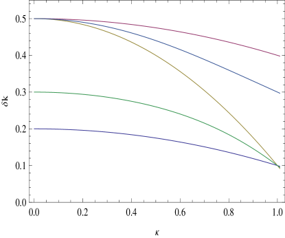
Figure 2: Spectrum of the five localized soliton eigenstates (13)-(17), representing their modulation wavectors as a function of $\kappa$. The bottom curve corresponds to the lowest soliton eigenstate and the top curve to the highest soliton eigenstate of the trapped probe.

Two most stricking features emerging from the graph, that traduce relevant physical implications of the variation of wavectors with $\kappa$ on the mode stability, are the decrease of their modulation wavectors when they decay from the wavetrain structure to their respective single fundamental-soliton states, and their degenerate features in the two limit values of $\kappa$. Recall that when $\kappa$ tends to zero, the Jacobi elliptic functions reduce to harmonic waves which are intrinsically linear.

3.2 The $|3,l\textgreater$ soliton modes

When $n=3$ the ratio of the XPM to the SPM coupling strengths takes the value $\beta=6\xi D$, corresonding to a stronger XPM effect exerted by the pump on the probe. The resulting spectral problem for the trapped probe now reads:

$$u_{\tau\tau}+\left[h(k)-12\kappa^{2}sn^{2}(\tau)\right]u=0.$$ (23)

For this spectral problem, the localized-mode spectrum bursts into seven different eigenstates given by [32]:
$|3,1\textgreater$ soliton mode:

$$u_{1}(\tau) = u_{1,0}(\kappa)\,\left[sn^{2}\left(\tau-\tau_{0}\right)-\frac{2(1+\kappa^{2})-\sqrt{4-7\kappa^{2}+4\kappa^{4}}}{5\kappa^{2}}\right]\,sn\left(\tau-\tau_{0}\right),$$

$$k_{1}(\kappa) = k_{\lambda}+\frac{Q^{2}D}{2}\left[7-5\kappa^{2}-2\sqrt{4-7\kappa^{2}+4\kappa^{4}}\right],$$ (24)

$|3,2\textgreater$ soliton mode:

$$u_{2}(\tau) = u_{2,0}(\kappa)\,\left[sn^{2}\left(\tau-\tau_{0}\right)-\frac{2+\kappa^{2}-\sqrt{4-\kappa^{2}(1-\kappa^{2})}}{5\kappa^{2}}\right]\,cn\left(\tau-\tau_{0}\right),$$

$$k_{2}(\kappa) = k_{\lambda}+\frac{Q^{2}D}{2}\left[7-2\kappa^{2}-2\sqrt{4-\kappa^{2}(1-\kappa^{2})}\right],$$ (25)

$|3,3\textgreater$ soliton mode:

$$u_{3}(\tau) = u_{3,0}\left[sn^{2}\left(\tau-\tau_{0}\right)-\frac{1+2\kappa^{2}-\sqrt{1-\kappa^{2}+4\kappa^{4}}}{5\kappa^{2}}\right]\,dn\left(\tau-\tau_{0}\right),$$

$$k_{3}(\kappa) = k_{\lambda}+\frac{Q^{2}D}{2}\left[10-5\kappa^{2}-2\sqrt{1-\kappa^{2}+4\kappa^{4}}\right],$$ (26)

$|3,4\textgreater$ soliton mode:

$$u_{4}(\tau) = u_{4,0}(\kappa)\,cn\left(\tau-\tau_{0}\right)\,dn\left(\tau-\tau_{0}\right)\,sn\left(\tau-\tau_{0}\right),$$

$$k_{4}(\kappa) = k_{\lambda}+2Q^{2}D(2-\kappa^{2}),$$ (27)

$|3,5\textgreater$ soliton mode:

$$u_{5}(\tau) = u_{5,0}(\kappa)\,\left[sn^{2}\left(\tau-\tau_{0}\right)-\frac{2(1+\kappa^{2})+\sqrt{4-7\kappa^{2}+4\kappa^{4}}}{5\kappa^{2}}\right]\,sn\left(\tau-\tau_{0}\right),$$

$$k_{5}(\kappa) = k_{\lambda}+\frac{Q^{2}D}{2}\left[7-5\kappa^{2}+2\sqrt{4-7\kappa^{2}+4\kappa^{4}}\right],$$ (28)

$|3,6\textgreater$ soliton mode:

$$u_{6}(\tau) = u_{6,0}(\kappa)\,\left[sn^{2}\left(\tau-\tau_{0}\right)-\frac{2+\kappa^{2}+\sqrt{4-\kappa^{2}(1-\kappa^{2})}}{5\kappa^{2}}\right]\,cn\left(\tau-\tau_{0}\right),$$

$$k_{6}(\kappa) = k_{\lambda}+\frac{Q^{2}D}{2}\left[7-2\kappa^{2}+2\sqrt{4-\kappa^{2}(1-\kappa^{2})}\right].$$ (29)

$|3,7\textgreater$ soliton mode:

$$u_{7}(\tau) = u_{7,0}(\kappa)\,\left[sn^{2}\left(\tau-\tau_{0}\right)-\frac{1+2\kappa^{2}+\sqrt{1-\kappa^{2}+4\kappa^{4}}}{5\kappa^{2}}\right]\,dn\left(\tau-\tau_{0}\right),$$

$$k_{7}(\kappa) = k_{\lambda}+\frac{Q^{2}D}{2}\left[10-5\kappa^{2}+2\sqrt{1-\kappa^{2}+4\kappa^{4}}\right],$$ (30)

Figures 3 and 4 depict temporal profiles of their intensities, for $\kappa<0.95$ (left graphs) and $\kappa=1$ (right graphs).

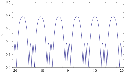
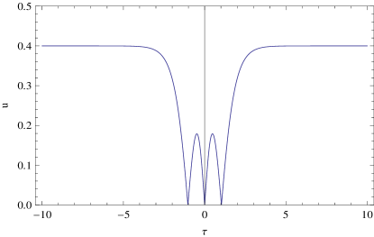
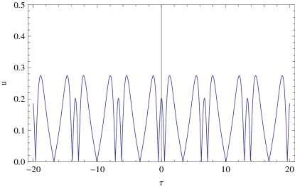
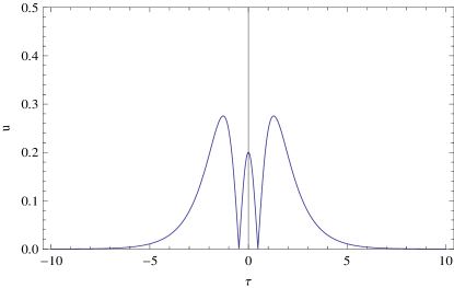
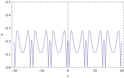
Figure 3: Intensities $|u(\tau)|$ of the soliton modes $|3,l\textgreater$ given by (24)-(26), for $\kappa=0.95$ (left graphs) and $\kappa=1$ (right graphs). Modes are displayed from the lowest (top graph) to the highest (bottom graph) soliton eigenstates in terms of their modulation wavectors.

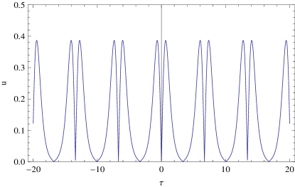
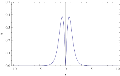
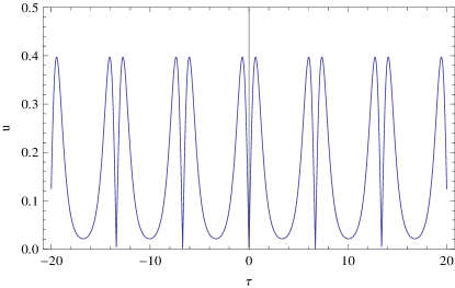
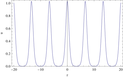
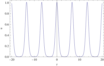
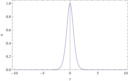
Figure 4: Intensities $|u(\tau)|$ of the soliton modes $|3,l\textgreater$ given by (27)-(30), for $\kappa=0.95$ (left graphs) and $\kappa=1$ (right graphs). Modes are displayed from the lowest (top graph) to the highest (bottom graph) soliton eigenstates in terms of their modulation wavectors.

Like in the previous case the seven localized probe modes are dominated by periodic wavetrain profiles, consisting of sequences of pulses of different periodicities when $\kappa<1$. From the right graphs we find that contrary to the previous case, three distinct fundamental soliton modes show up when the XPM strength is higher namely single-pulse, double-pulse and tripple-pulse periodic wavetrains. Their analytical expressions are derived from (24)-(30) for $\kappa\rightarrow 1$ and are explicitely given by:

$$u_{1}(\tau) \propto \left[2-5\,sech^{2}\left(\tau-\tau_{0}\right)\right]\,tanh\left(\tau-\tau_{0}\right),$$

$$k_{1} = k_{\lambda},$$ (31)

$$u_{2}(\tau) \propto \left[4-5\,sech^{2}\left(\tau-\tau_{0}\right)\right]\,sech\left(\tau-\tau_{0}\right),$$

$$k_{2} = k_{\lambda}+\frac{Q^{2}D}{2},$$ (32)

$$u_{3}(\tau) \propto \left[4-5\,sech^{2}\left(\tau-\tau_{0}\right)\right]\,sech\left(\tau-\tau_{0}\right),$$

$$k_{3} = k_{\lambda}+\frac{Q^{2}D}{2},$$ (33)

$$u_{4}(\tau) \propto sech^{2}\left(\tau-\tau_{0}\right)\,tanh\left(\tau-\tau_{0}\right),$$

$$k_{4} = k_{\lambda}+2Q^{2}D,$$ (34)

$$u_{5}(\tau) \propto sech^{2}\left(\tau-\tau_{0}\right)\,tanh\left(\tau-\tau_{0}\right),$$

$$k_{5} = k_{\lambda}+2Q^{2}D,$$ (35)

$$u_{6}(\tau) \propto sech^{3}\left(\tau-\tau_{0}\right),$$

$$k_{6} = k_{\lambda}+\frac{9Q^{2}D}{2},$$ (36)

$$u_{7}(\tau) \propto sech^{3}\left(\tau-\tau_{0}\right),$$

$$k_{7} = k_{\lambda}+\frac{9Q^{2}D}{2}.$$ (37)

Figure 5 displays the spectrum of the seven localized soliton modes, more precisely here are plotted their modulation wavectors versus $\kappa$.

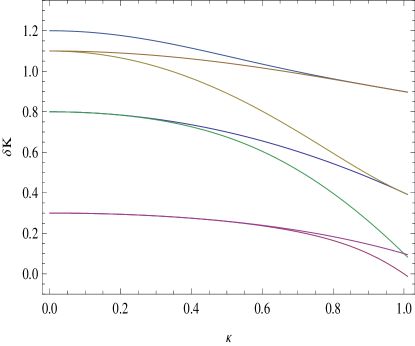
Figure 5: Spectrum of the seven localized soliton eigenstates (24)-(30), representing their modulation wavectors as a function of $\kappa$. The bottom curve corresponds to the lowest soliton eigenstate and the top curve to the highest soliton eigenstate of the trapped probe.

Like the first case studied in the previous section, the modulation wavectors decrease from a high-momentum excitation regime where the seven probe soliton modes collapse into degenerate linear waves, to a low-momentum excitation regime where they reduce to their characteristic fundamental soliton modes. Also remarkable are mode degeneracies, in this case we notice that the number of degenerate modes is higher and is expected to increase with increasing value of the ratio of the XPM to the SPM coupling strengths.

4 conclusion

The induced-phase-modulation (or cross-phase-modulation) process has been predicted two decades ago [1, 2, 9, 10], and experimentally observed [3, 4] to occur when a low-power signal (either an harmonic cw signal or a weakly nonlinear signal) couples to a high-intensity pump signal, the later one providing an optical waveguiding structure and reshaping channel to the first for substantial increase of its lifetime. However while this process is rather well understood for single-soliton pumps and in the case of relatively weak cross-phase-modulation processes, almost no insight exists about the context of pump signals consisting of periodic networks of temporal or spatial solitons [18]. The main objective of this work was to point out the great variety of spectral properties of pure harmonic cw probes trapped by a pump field consisting of a periodic wavetrain of optical pulses, when different orders of magnitudes of the cross-phase-modulation coupling are considered for the same self-phase-modulation coupling strength. The principal motivation for carrying out such analysis is the broad range of technological applications behind the possibility to combine, both quantitatively and qualitatively, multi-color soliton signals generated from on single pump field. On the other hand, the very large diversity of physical properties expected from optical materials that can be fabricated via current technological means, makes it hard to think of physical contexts where cross-phase-modulation processes will always be far weaker than the intrinsic nonlinearity of pump fields. From these last standpoints the present study provides new interesting insight onto the general physics of pump-probe systems. In particular the increasingly large number and variety of possible soliton modes induced by the soliton pump for relatively strong cross-phase-modulation proceses, offers new opportunity to create multi-component vector solitons from optical low-power optical fields via light-induced waveguiding phenomena, thus enriching current designs of engineered (i.e. artificially created) soliton networks from reconfigurable non-soliton signals by means of all-optical techniques. To end, we wish to underline the richness of the fundamental modes emerging from the present study with increasing cross-phase-modulation coupling strength, for a fixed strength of the self-phase-modulation effect. While some of these modes have already been predicted [2, 9], in the present and our recent [18] works their spectral properties, conditions of existence as well as stability have been formally established. The key insight about these fundamental modes is that they put into play multi-pulse structures that are generated from the same pump, but with different modulation wavectors and hence different instantaneous wavelengths.

References

References

- [1] Manassah J T 1990 Ultrafast solitary waves sustained through induced phase modulation by a copropagating pump Opt. Lett. 15 670-672.
- [2] Manassah J T 1991 Induced waveguiding effects in a two-dimensional nonlinear medium Opt. Lett. 16 587-589.
- [3] De La Fuente R, Barthelemy A and Froehly C 1991 Spatial-soliton-induced guided waves in a homogeneous nonlinear Kerr medium Opt. Lett. 16 793-795.
- [4] de la Fuente R and Barthelemy A 1992 Spatial soliton-induced guiding by cross-phase modulation IEEE J. Quantum Electron. 28 547-554.
- [5] Tomlinson W J, Stolen R H and Johnson A M 1985 Optical wave breaking of pulses in nonlinear optical fibers Opt. Lett. 10 457-459.
- [6] Agrawal G P, Baldeck P L and Alfano R R 1989 Optical wave breaking and pulse compression due to cross-phase modulation in optical fibers Opt. Lett. 14 137-139.
- [7] Ostrovskaya E A, Kivshar Yu S, Skryabin D V and Firth W J 1999 Stability of multihump optical solitons Phys. Rev. Lett.83 296-299.
- [8] Shipulin A, Onishchukov G and Malomed B A 1997 Suppression of soliton jitter by a copropagating support structure J. Opt. Soc. Am.B14 3393-3402.
- [9] Steiglitz K and Rand D 2009 Photon trapping and transfer with solitons Phys. Rev.A79 0218021-4(R).
- [10] Steiglitz K 2010 Soliton-guided phase shifter and beam splitter Phys. Rev.A81 0338351-5.
- [11] Eugenieva E D, Efremidis N K and Christodoulides D N 2001 Design of switching junctions for two-dimensional discrete soliton networks Opt. Lett. 26 1978-1980.
- [12] Fleischer J W, Carmon T, Segev M, Efremidis N K and Christodoulides D N 2003 Observation of discrete solitons in optically induced real time waveguide arrays Phys. Rev. Lett.90 0239021-4.
- [13] Fleischer J W, Segev M, Efremidis N K and Christodoulides D N 2003 Observation of two-dimensional discrete solitons in optically induced nonlinear photonic lattices Nature 422 147-150.
- [14] Neshev D, Sukhorukov A, Kivshar Yu S, Ostrovskaya E and Krolikowski W 2003 Discrete solitons in light-induced index gratings Opt. Lett. 28 710-712.
- [15] Martin H, Eugenieva E D, Chen Z and Christodoulides D N 2004 Discrete solitons and soliton-induced dislocations in partially-coherent photonic lattices Phys. Rev. Lett.92 1239021-4.
- [16] Cartaxo A V T 1999 Cross-phase modulation in intensity modulation-direct detection WDM systems with multiple optical amplifiers and dispersion compensators J. Lightwave Technol. 17 178-190.
- [17] Naumov A N and Zheltikov A M 2000 Cross-phase modulation in short light pulses as a probe for Gas ionization dynamics: the influence of group-delay walk-off effects Laser Physics 10 923-926.
- [18] Dikandé A M 2010 Fundamental modes of a trapped probe photon in optical fibers conveying periodic pulse trains Phys. Rev.A81 0136211-5.
- [19] Chen Z and Martin H 2003 Waveguides and waveguide arrays formed by incoherent light in photorefractive materials Optical Materials 23 235-241.
- [20] Islam M N, Mollenauer L F, Stolen R H, Simpson J R and Shang H T 1987 Cross-phase modulation in optical fibers Opt. Lett. 12 625-627.
- [21] Shapiro J H and Bondurant R S 2006 Qubit degradation due to cross-phase-modulation photon-number measurement Phys. Rev.A73 0223011-4.
- [22] Shapiro J H 2006 Single-photon Kerr nonlinearities do not help quantum computation Phys. Rev.A73 0623051-11.
- [23] Lan S, DelRe E, Chen Z, Shih M F and Segev M 1999 Directional coupler using soliton-induced waveguides Opt. Lett. 24 475-477.
- [24] Golovchenko E A, Pilipetskii A N and Menyuk C R 1996 Minimum channel spacing in filtered soliton wavelength-division-multiplexing transmission Opt. Lett. 21 195-197.
- [25] Wai P K A, Menyuk C R and Raghavan B 1996 Wavelength division multiplexing in an unfiltered soliton communication system J. Lightwave Technol. 14 1449-1454.
- [26] Del Duce A, Killey R I and Bayvel P 2004 Comparison of nonlinear pulse interactions in 160-Gb/s quasi-linear and dispersion managed soliton systems J. Lightwave Technol. 22 1263-1271.
- [27] Hansen E R 1975 A Table of Series and Products, Prentice-Hill Inc, Englewood Cliffs(N. J.).
- [28] Magnus W, Oberhettinger F and Tricomi F G 1953 Handbook of Transcendental Functions (McGraw Hill, New York)
- [29] Aleshkevich V, Kartashov Y and Vysloukh V 2001 Self-frequency shift of cnoidal waves in a medium with delayed nonlinear response J. Opt. Soc. Am.B18 1127-1136.
- [30] Kartashov Y, Aleshkevich V, Vysloukh V, Egorov A A and Zelenina A S 2003 Stability analysis of -dimensional cnoidal waves in media with cubic nonlinearity Phys. Rev.E67 0366131-11.
- [31] Dikandé A M 1999 Bound States in One-dimensional Klein-Gordon systems admitting periodic-kink soliton excitations Phys. Scr.60 291-293.
- [32] Arscott F M 1964, Periodic Differential equations: An introduction to Mathieu, Lamé and Allied Functions (Pergamon Press LTD)