Chronology protection and the stringy exclusion principle

Abstract:

We construct a family of supersymmetric solutions to AdS supergravity in three dimensions, that correspond to type IIB seven branes wrapped on an internal S${}^{3}\times$T⁴. These solutions are generalizations of the three dimensional Gödel universe and have closed timelike curves. We propose a enhançon-like mechanism for excising the closed timelike curve region by including the effects of additional light degrees of freedom. These take the form of tensionless 7-brane probes, effectively described through the backreaction of a smeared domain wall. The absence of closed timelike curves in the asymptotic AdS₃ geometries obtained in this way is shown to be equivalent to a unitarity bound in the dual CFT, known as the stringy exclusion principle.

1 Introduction

One of the more dramatic consequences of the intrinsic connection between gravity and the geometry and causal structure of space-time, is the possible appearance of closed timelike curves (CTCs). The textbook example of how even a simple, at first sight completely physical, distribution of energy momentum can lead to CTCs, is the metric presented by Kurt Gödel in 1949 [1]. His solution to Einstein’s equations is a product of a line and a three-dimensional spacetime with nontrivial metric

$$\frac{ds^{2}}{l^{2}}=-\left(dt+\mu\frac{r^{2}}{1-r^{2}}d\phi\right)^{2}+\mu\frac{dr^{2}+r^{2}d\phi^{2}}{(1-r^{2})^{2}}.$$ (1)

The latter is a solution of three dimensional gravity with negative cosmological constant $\Lambda=-1/l^{2}$ and a source of pressureless rotating dust. The parameter $\mu$ is greater than one and is related to the density of the dust as $\mu=1/(1-\rho)$. The metric can be viewed as timelike stretched $AdS_{3}$, where $\mu$ plays the role of the stretching factor [2]. It is easily seen that the $\phi$-circles are CTCs in the region $1/\sqrt{\mu}<r\leq 1$. For more details on the Gödel geometry, see e.g. [3].

Apart from this famous example, many more classical solutions with CTCs are currently known, including supersymmetric versions in supergravity theories, both in 3+1 dimensions as well as in their higher-dimensional parent theories (examples include [4],[5],[6]). Such spacetimes lead to a variety of pathologies, both within classical general relativity as well as for interacting quantum fields propagating on them (see [7] for a review and further references). This led Hawking to propose the Chronology Protection Conjecture, stating that regions containing CTCs cannot be formed in any physical process [8]. Although he was able to provide a proof in the classical theory, his assumptions are violated once quantum effects are taken into account. As argued in e.g. [9] one expects a fully consistent treatment of chronology protection to require a theory where gravity itself is quantized.

Providing such a quantum description of gravity, the AdS/CFT correspondence [10] is a promising tool for studying chronology protection, at least in asymptotically AdS spaces. As illustrated by the above example, the appearance of CTCs is often a subtle global or IR feature in the bulk, which, because of UV/IR connection in AdS/CFT [11], can be expected to appear as a more obvious UV problem in the dual CFT. This idea seems to be borne out in a number of examples, where the appearance of CTCs in the bulk corresponds to an obvious violation of unitarity bounds in the dual CFT [12, 13, 14, 15]. Therefore it seems that, if the underlying quantum gravity theory is unitary, the geometries containing CTCs are unphysical and cannot be formed in any process.

In [16], we demonstrated such a link between chronology protection and unitarity in a very simple model where only some very basic features of quantum gravity in asymptotic AdS-space were assumed. The setup was as follows. We computed the backreaction of a spinning ball of dust, of radius $r_{0}$ and density $\rho$, in three dimensional gravity. Within the dust ball, the metric is the Gödel metric (1) for $r\leq r_{0}$. Outside of the ball of dust, where there is no stress-energy, the metric is a generalized BTZ metric [17, 18]. Such metrics depend on two real parameters, the ADM mass $M$ and angular momentum $J$:

$${ds^{2}\over l^{2}} = -(u-M)d\tilde{t}^{2}-Jd\tilde{t}d\tilde{\phi}+ud\tilde{\phi}^{2}+{du^{2}\over 4f(u)}\,,$$ (2)

$$f(u) = u^{2}-Mu+{J^{2}\over 4}\,.$$

The Israel matching conditions relate the values of $M$ and $J$ to that of the dust ball, $\rho$ and $r_{0}$. It turns out the for this matched solution $M$ and $J$ always satisfy $|J|>M$, in which case the metric has no horizons, see figure 1.

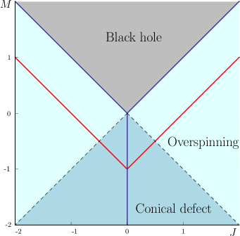
Figure 1: The BTZ metrics (2) fall in three different classes, depending on the relative values of the mass $M$ and angular momentum $J$. The metric describes a black hole when $M>|J|$, a naked conical defect when $M<-|J|$ or is free of horizons and singularities when it is overspinning, i.e. $|M|<|J|$. All metrics above the red lines $M+1=|J|$ have positive conformal weights, while metrics below don’t. Asymptotic metrics originating from a matching onto a part of Gödel space (1) all fall either in the class of the conical defects or the overspinning class. Considered as complete metrics on their own these spaces have naked CTCs with the exception of ones lying on the blue lines.

For $u<0$ the $\tilde{\phi}$ circle in (2) is timelike. Closed timelike curves will be present in the combined spacetime only if the value of the radius $r_{0}$ where the two metrics (1) and (2) are glued together, exceeds the critical value $\frac{1}{\sqrt{\mu}}$, which corresponds to $u_{0}=0$ in the BTZ metric.

It was our observation in [16] that, in the two parameter family of solutions thus obtained, the solutions with CTCs would precisely correspond to states with negative conformal weight and are hence excluded in a unitary theory.

In this work, we will clarify and extend this simple model in several ways. We start by embedding our model into string theory, and provide a D-brane interpretation of the Gödel universe, building on [6]. We consider type IIB compactifications on $S^{3}\times T^{4}$, with 7-branes wrapping the internal manifold. We include in our discussion the 7-branes producing general SL(2,$\mathbb{Z}$) monodromy that were called Q7- branes in [19], [20]. The backreaction of these 7-branes produces orbifolds of Gödel space which we construct explicitly. These solutions are the analog of the ones considered in [19], [20] in the presence of a negative cosmological constant, and are D-brane realizations of the ‘Gödel cosmons’ discussed in [21].

In the second part of the paper, we propose a dynamical mechanism for the excision of the region in Gödel space that contains closed timelike curves. In string theory, singularities in the effective supergravity description can often be shown to be artifacts of the low-energy limit which are resolved when carefully taking into account the dynamics of the full underlying theory. The mechanism for resolution often involves the inclusion of nonperturbative degrees of freedom that become light in the problematic region of spacetime and should be included in the effective description. Such objects will tend to condense at the locus where their tension becomes zero, effectively forming a domain wall which excises the spacetime singularity. A well-understood example of such a resolution mechanism is the excision of repulson singularities [22]. In that example, the branes that produce the supergravity background are, when considered as probes, found to become tachyonic in a region of space surrounding the singularity. On the locus where the tachyonic instability appears, these branes are tensionless, and thus provide additional massless modes that should be included in the low energy description. An effective description of this effect is to consider a thin shell of smeared branes on this locus, its backreaction leaves a regular geometry inside the shell and excises the repulson singularity.

When the supergravity solution contains, instead of a curvature singularity, a region with closed timelike curves, a similar mechanism was conjectured to apply in [23], and a five-dimensional example was given. Such examples are very interesting as they provide hints at what may eventually become a proof of Hawking’s chronology protection conjecture in a UV complete theory of quantum gravity such as string theory.

We propose a dynamical resolution of the closed timelike curve region of Gödel space, very much along the lines of [23]. We begin by identifying Q7-brane probes that become light in a region of Gödel space. We assume that they condense at the critical radius where they become exactly massless, forming a supersymmetric domain wall consisting of branes smeared on this radius. We then show that this mechanism is consistent in supergravity by finding the precise solution on the outside of the domain wall that satisfies the Israel matching conditions and show that the complete matched spacetime is globally supersymmetric, i.e. the Killing spinors are analytic through the domain wall. The outside metric turns out to be a spinning supersymmetric BTZ solution corresponding to chiral primary states in the dual CFT. Our proposal is therefore also interesting from the point of view of the outside geometry, as it removes the CTC region of the spinning BTZ metric near its core, replacing it with a harmless patch of the Gödel universe.

One new feature of our example is that we find a discrete family of such matched solutions, parameterized by the total R-charge they carry. For a certain range of values of the R-charge, the matched spacetime is free of CTCs. One very interesting feature, which we take as strong evidence that our proposed excision mechanism is consistent, is that this range of R-charges precisely reproduces the unitarity bounds on chiral primaries. That is, not only do we recover the bound that the conformal weight is positive definite, but we also reproduce the upper bound on the conformal weight which is known as the stringy exclusion principle [25] and is hard to derive from the bulk point of view.

This paper is structured as follows. First, in section 2, we review the (2,0) AdS supergravity theory which will be our framework, and we discuss the supersymmetric particle actions that couple to this theory. In section 3 we then exhibit a number of supersymmetric solutions. There is a family of solutions corresponding to the backreaction of wrapped 7-branes, all locally Gödel, and we point out which configuration corresponds to global Gödel space. Finally we also review the supersymmetric vacuum solutions and their relation to chiral primaries in the bulk. In section 4 we present our main results. First we discuss 7-brane probes and how they can become massless in the Gödel background and then we show in detail how the backreaction of such probes smeared into a domain wall leads to an asymptotic AdS₃ space. Furthermore we show that the combined spacetime is globally supersymmetric. We then analyze the discrete family of solutions obtained and show the equivalence between absence of closed timelike curves and unitarity in the dual CFT. We conclude and point to some interesting remaining questions in section 5. For the readers convenience we included a number of technical appendices. In appendix A we detail the reduction of type IIB and its 7-branes to 3 dimensions. In appendix B we provide the details on solving the relevant Killing spinor equations and in C on solving the Israel matching conditions.

2 AdS supergravity with axion-dilaton

In this section we review the properties of $(2,0)$ AdS supergravity in three dimensions with an axion-dilaton matter field. Although we adopt this three dimensional supergravity point of view throughout most of the paper, our main interest in this system is as a limit of string theory. The embedding into string theory requires certain quantization conditions on the couplings and charges in the supergravity theory. We will keep track of these quantization conditions along the way, but the reader interested in purely classical supergravity applications may safely ignore them. We refer to Appendix A for explicit details on how this theory, and hence its solutions, can be obtained as a consistent reduction and truncation of Type IIB string theory, note that some more comments on the U-dualities that connect this setup to Type IIA and M-theory embeddings can be found in [6].

2.1 Three dimensional (2,0) AdS supergravity

It is well known [27, 28] that in three dimensions Einstein gravity with a negative cosmological constant can be rewritten as a Chern-Simons theory for the non-compact gauge group SL(2,$\mathbb{R}$)${}_{L}\times$SL(2,$\mathbb{R})_{R}$. One can generalize this construction to supergravities by replacing the gauge group by a supergroup. This leads to the ($p,q$) AdS supergravities of [27, 29], defined as the Chern-Simons theory of the group OSp($p|2,\mathbb{R})_{L}\times$OSp($q|2,\mathbb{R})_{R}$. These are pure, or minimal, supergravities in that they only contain the graviton multiplet. The $(4,4)$ and $(4,0)$ cases are familiar, as they describe the gravity multiplet of the well known AdS/CFT examples for AdS${}_{3}\times$S³ and AdS${}_{3}\times$S² respectively [30]. In general one can couple sigma-model matter to these theories, but to the authors’ knowledge this coupling has not been worked out in detail for general $(p,q)$. The $(2,0)$ case has however been studied in some detail [31], and as such we find it convenient to work in this setup as it is the minimal one that contains the ingredients we need. Note that the embedding in string theory is most naturally connected to the $(4,0)$ and $(4,4)$ theories, see appendix A for some details, but the $(2,0)$ truncation contains the subsector of our interest.

In $(2,0)$ AdS supergravity the gravity multiplet contains not only the graviton $g_{\mu\nu}$, but also a $U(1)$ Chern-Simons gaugefield $A^{L}$. Furthermore we can couple it to a scalar matter multiplet, where supersymmetry demands this sigma model matter to have a target space that is Kähler. Denoting the space-time pullback of the target space vielbein by ${}^{*}{{\cal P}}$, the bosonic part of the action of this theory is [31]:

$$S_{\mathrm{grav}}={1\over 16\pi G}\int_{{\cal M}_{3}}d^{3}x\left[\sqrt{-g}\left(R+\frac{2}{l^{2}}-2(\mu-1){}^{*}{{\cal P}}_{\alpha}{}^{*}\bar{{\cal P}}^{\alpha}\right)-{2\over l}\epsilon^{\alpha\beta\gamma}A^{L}_{\alpha}\partial_{\beta}A^{L}_{\gamma}\right]\,.$$ (3)

Note that we introduced a constant $\mu\geq 1$ to parameterize the coupling between matter and gravity which, for our embedding in type IIB string theory discussed in appendix A, should be taken to be $\mu=3/2$.

The fermionic variations under supersymmetry lead to the following conditions for a bosonic field configuration to be supersymmetric:

$$\left(\partial_{\alpha}+B^{L}_{\alpha\hat{\beta}}\gamma^{\hat{\beta}}-{i\over l}A^{L}_{\alpha}-{i\over 2}(\mu-1)\;^{*}{\cal Q}_{\alpha}\right)\epsilon = 0\,,$$ (4)

$$(\mu-1)\;^{*}{{\cal P}}_{\alpha}\gamma^{\alpha}\epsilon\ = 0\,.$$ (5)

Here we have introduced the left gravitational Chern-Simons connection $B^{L}$:

$$B^{L}_{\alpha\hat{\beta}}={1\over 4}\omega_{\alpha}^{\ \hat{\gamma}\hat{\delta}}\epsilon_{\hat{\gamma}\hat{\delta}\hat{\beta}}-{1\over 2l}e_{\alpha\hat{\beta}}\,.$$ (6)

Furthermore ${}^{*}{\cal Q}$ is the pull-back to space-time of a natural connection defined on the scalar target space. Given a Kähler potential ${\cal K}$, one can construct the Kähler connection ${\cal Q}$ as:

$${\cal Q}=\frac{i}{4}(\partial{\cal K}-\bar{\partial}{\cal K})\,.$$ (7)

Finally note that $\epsilon$ is a complex 2-component spinor and hatted indices are frame indices.

The case we are interested in is when the scalar target space is the coset SL(2,$\mathbb{R}$)/SO(2). The vielbein and Kähler connection can in this case be written as

$${\cal K} = 4\ln{\rm Im}\tau$$ (8)

$${{\cal P}} = \frac{1}{\sqrt{2}}\frac{d\tau}{\mathrm{Im}\tau}$$ (9)

$${\cal Q} = \frac{d\mathrm{Re}\tau}{\mathrm{Im}\tau}\,,$$ (10)

where $\tau$ is a complex scalar taking values on the upper half plane: $\mathrm{Im}\tau>0$. The scalar kinetic term in the action becomes:

$$-2(\mu-1){}^{*}{{\cal P}}_{\alpha}{}^{*}\bar{{\cal P}}^{\alpha}=-(\mu-1)\frac{\partial_{\alpha}\tau\partial^{\alpha}\bar{\tau}}{({\rm Im}\tau)^{2}}\,.$$ (11)

When we think of the 3 dimensional theory as originating from a compactification of IIB string theory, see appendix A, the scalar $\tau$ is the familiar axion-dilaton of the IIB theory. In string theory the continues SL(2,$\mathbb{R}$) symmetry is broken by quantization conditions to the discrete subgroup SL$(2,\mathbb{Z})$.

2.2 Supersymmetric particles

Given the framework of the (2,0)-supergravity, we will be interested in the supersymmetric charged particles that one can couple to this theory. A particle in 3 dimensions, just as any codimension 2 object, will backreact strongly on space-time, introducing a conical defect proportional to its mass [32, 33]. In this subsection we discuss the source terms corresponding to such point masses, and two ways to couple them to the other background fields in a supersymmetric fashion.

2.2.1 R-particles

The first type of supersymmetric particle is probably the most familiar, [31, 34, 35, 36]. It is a particle that is electrically charged under the U(1) CS gaugefield $A^{L}$, with a mass equal to its charge. Since in the dual CFT such particle states are characterized by non vanishing R-charge, we will refer to them as R-particles. In the higher dimensional picture the U(1) gauge symmetry corresponds to a rotation of a sphere factor in the compactification manifold, and from this point of view the R-charge is interpreted as angular momentum. The bosonic part of the action for such supersymmetric particles is simply given by:

$$S_{R}=-\frac{b}{4G}\int\left(\sqrt{-g}-A^{L}\right)\,.$$ (12)

In an embedding in string theory the charge $b$ is quantized as $b=R\frac{4G}{l}=\frac{R}{N^{2}}$. As detailed in appendix A, $N$ is related to the five form flux on the internal space, and is quantized to be integer, and $R$ corresponds to R-charge in the dual field theory and is also naturally quantized in integer units.

2.2.2 Q-particles

A second type of supersymmetric particle carries magnetic charge under an axionic scalar of the sigma-model matter. Supersymmetry requires that the particle mass depends on the other real scalar comprising the complex axion-dilaton. In terms of the higher dimensional IIB origin of the (2,0) supergravity (see appendix A), this type of supersymmetric particle corresponds to a 7-brane wrapping the complete 7 dimensional internal space. There is a large class of different supersymmetric 7-branes, classified in the ten dimensional setting by [19]. Each of them is magnetically charged under a different axionic scalar. The most familiar one is the D7 brane which is magnetically charged under $\mathrm{Re}\tau$, and produces a monodromy $\tau\rightarrow\tau+1$. As [19] showed, more generally there exists a supersymmetric 7-brane associated to any SL(2,$\mathbb{Z}$) monodromy $e^{Q}$, and the different branes, or particles from the three dimensional standpoint, can thus be classified by the Lie algebra element:

$$Q=\begin{pmatrix}\frac{r}{2}&p\\ -q&-\frac{r}{2}\end{pmatrix}\,.$$ (13)

The axion $a_{Q}$ these particles couple to is a target space coordinate along the integral curves of the Killing vector associated to $Q$:

$$k_{Q}=\mathrm{Re}\left[(p+r\tau+q\tau^{2})\partial_{\tau}\right]\equiv\partial_{a_{Q}}\,.$$ (14)

Each of these axions $a_{Q}$ is most naturally interpreted as the real part of a complex scalar $\upsilon_{Q}$, i.e. $a_{Q}=\mathrm{Re}\,\upsilon_{Q}$. Integrating the condition (14) then gives (assuming $\det Q\geq 0$):

$$\begin{cases}\tau=-\frac{r}{2q}-\frac{\sqrt{\det Q}}{q}\cot\left(\sqrt{\det Q}\,\upsilon_{Q}\right)\qquad\mbox{when }q>0\\ \tau=p\upsilon_{Q}\ \ \,\quad\qquad\qquad\qquad\qquad\qquad\quad\,\,\,\mbox{when }q=r=0\,.\end{cases}$$ (15)

In terms of the new coordinate, a convenient choice of the target space Kähler potential, U(1)-connection and vielbein is

$${\cal K} = 4\ln\sinh\left(2\sqrt{\det Q}{\rm Im}\upsilon_{Q}\right)\,,$$ (16)

$${\cal Q} = {2\sqrt{\det Q}d{\rm Re}\upsilon_{Q}\over\tanh\left(2\sqrt{\det Q}{\rm Im}\upsilon_{Q}\right)}\,,$$ (17)

$${{\cal P}} = {\sqrt{2\det Q}d\lambda\over\sinh\left(2\sqrt{\det Q}{\rm Im}\upsilon_{Q}\right)}\,.$$ (18)

The supersymmetric couplings of a Q-particle were worked out in [19, 20]. The tension of the brane (mass of the particle in three dimensions) is related to the imaginary part of the new complex scalar $\upsilon_{Q}$ :

$$T_{Q}=\frac{p+r\mathrm{Re}\tau+q|\tau|^{2}}{\mathrm{Im}\tau}=2\sqrt{\det Q}\coth\left(2\sqrt{\det Q}\mathrm{Im}\,\upsilon_{Q}\right)\,.$$ (19)

The bosonic part of the Q-particle action is given by:

$$S_{Q}=-\frac{(\mu-1)}{8\pi G}\int\left(T_{Q}\sqrt{-g}-C_{Q}\right)$$ (20)

where $C_{Q}$ is the potential of the fieldstrength $G_{Q}=dC_{Q}$, dual to the axion:

$$G_{Q}=\left(T^{2}_{Q}-4\det Q\right)\star\!da_{Q}\,.$$ (21)

It is often useful to work not in terms of the complex scalar $\tau$, but directly in terms of the fields the Q-particle most naturally couples to. So we rewrite the SL(2,$\mathbb{R}$)/SO(2) coset action as an equivalent action in terms of the scalar tension $T$, and the gaugefield $C$ (where from now on we will imagine working with a given charge $Q$ and suppress it as an index):

$$S=-\frac{(\mu-1)}{16\pi G}\int\sqrt{-g}\,dx^{3}\,\frac{\partial_{\mu}T\partial^{\mu}T+\frac{1}{2}G_{\mu\nu}G^{\mu\nu}}{T^{2}-4\det Q}\,.$$ (22)

Finally, let us comment on the relation to the more common ($p,q$)-branes. As the charge matrix $Q$ can be thought of as an element of the Lie-algebra, it transforms in the adjoint representation under SL(2,$\mathbb{Z}$) duality. The duality orbits are the SL(2,$\mathbb{Z}$) conjugacy classes and are determined by the value of $\det Q$. The requirement that $e^{Q}$ is an SL(2,$\mathbb{Z}$)-element, leads to the condition that $2\cos(\sqrt{\det Q})\in\mathbb{Z}$, or in other words: $\sqrt{\det Q}$ is an integer multiple of either $\pi/3$ or $\pi/2$. Up to an overall rescaling of $Q$, which labels the quantity of charge, the two physically different cases that arise in string theory are $\det Q=0$ and $\det Q=\pi^{2}$. The case $\det Q<0$ was argued in [19, 20] to be unphysical and we will not consider it here. The $\det Q=0$ particle corresponds to a parabolic conjugacy class and contains the D7 brane and all its SL(2,$\mathbb{Z}$) images, known as ($p,q$)-branes. The axion it couples to is generated by an $\mathbb{R}$ subgroup. The $\det Q=\pi^{2}$ particle corresponds to an elliptic conjugacy class and is not not connected to the D7 brane by U-duality. It couples to an axion that generates an SO(2) subgroup. This class contains objects which can be present in F-theory compactifications and can be interpreted in terms of bound states of D7-branes and O7 orientifold planes. The most familiar example of this last type, which will also appear in out setup, is the bound state of 4 D7 branes with an O7 orientifold plane [37], which has monodromy $-1$, and corresponds to $p=q=\pi,r=0$.

2.2.3 RQ-particles

Because the R- and Q-particles introduced above are mutually supersymmetric, one can also write down a supersymmetric action for a particle that is both charged under an axion, as well as under the CS gaugefield, which we will refer to as an ‘RQ-particle’ in what follows. From [38, 31] one can obtain the supersymmetry transformations of the relevant background bosonic fields, i.e the space-time dreibein $e^{a}$, the CS field $A^{L}$ and $C$, the U(1) dual of the axion:

$$\delta_{\epsilon}e^{a}_{\mu} = i\bar{\epsilon}\gamma^{a}\psi_{\mu}+\mathrm{c.c.}\,,$$ (23)

$$\delta_{\epsilon}A^{L}_{\mu} = \bar{\epsilon}\psi_{\mu}+\mathrm{c.c.}\,,$$ (24)

$$\delta_{\epsilon}C_{\mu} = T(\tau)(\bar{\epsilon}\psi_{\mu}+\mathrm{c.c.})+\mbox{terms involving the scalarino }\lambda\,.$$ (25)

As the three fields all have a variation proportional to the gravitino $\psi_{\mu}$, the couplings of the particle to these three background fields are linked in the $\kappa$-symmetry analysis of the particle action. The result is that the relative sign of the R- and Q- charge is fixed for a supersymmetric particle:

$$S_{RQ}=-\frac{1}{8\pi G}\int\Big{(}(\mu-1)T+2\pi b)\sqrt{-g}-(\mu-1)C-2\pi bA^{L}\Big{)}\,.$$ (26)

This way of giving R-charge to the Q-particles might seem a little ad hoc. However, by considering the geometries resulting from the backreaction of such RQ-particles on the metric, we show in the following section that for supersymmetric solutions such combined couplings are actually required. This effect is absent in flat space. It would be very interesting if there is a more natural worldvolume explanation of the coupling of the Q-particles to the CS gaugefield, perhaps through couplings with a worldvolume gaugefield, or through the curvature of the compactification manifold [20].

3 Supersymmetric solutions

In this section we construct supersymmetric solutions to the (2,0)-supergravity model. We begin by presenting the solutions that represent the backreaction of general RQ-particle sources. In particular, we will find that the Gödel metric discussed in the Introduction, when accompanied by a suitable Wilson line for the Chern-Simons gauge field, arises from the backreaction of a RQ-particle of charge $(\pi,\pi,0)$. We also show that the backreaction of a ‘common’ D7 brane is a certain orbifold of Gödel space. We end with a review on which subset of the BTZ metrics discussed in the Introduction can be viewed as BPS solutions to (2,0)-supergravity, and discuss their interpretation in the dual CFT.

3.1 Backreacted RQ-particles

In [6] it was shown that there exists a family of supersymmetric solutions to the theory (3). We shortly review those results here and furthermore consider the effect of including the supersymmetric sourceterms (26). For a supersymmetric solution it is natural to make a stationary ansatz for the metric where time is fibered over a 2-dimensional base manifold:

$$\frac{ds^{2}}{l^{2}}=-(dt+{\chi})^{2}+e^{2\varphi}dzd\bar{z}\,.$$ (27)

3.1.1 Equations of motion

Under this ansatz the equations of motion simplify drastically. Choosing the source (26) to be static with respect to $t$ and located at $z=0$, one finds the following equations [6, 19]:

$$\partial\bar{\partial}\tau+i\frac{\partial\tau\bar{\partial}\tau}{\mathrm{Im}\tau} = -\frac{i\pi}{4}\delta(z,\bar{z})(p+r\tau+q\tau^{2})\,,$$ (28)

$$\partial\bar{\partial}\varphi-e^{2\varphi} = -\frac{\mu-1}{4}\frac{\partial\tau\bar{\partial}\bar{\tau}}{(\mathrm{Im}\tau)^{2}}-\frac{1}{4}\left((\mu-1)T+2\pi b\right)\delta(z,\bar{z})\,,$$ (29)

$$d{\chi} = \frac{i}{2}e^{2\varphi}dz\wedge d\bar{z}\,,$$ (30)

$$\frac{1}{l}dA^{L} = \frac{i\pi}{2}b\delta(z,\bar{z})dz\wedge d\bar{z}\,.$$ (31)

These equations have a natural geometric interpretation in the F-theory embedding of our system. Let us first discuss the equations in the absence delta-function sources. The first two equations describe the geometry of the four-dimensional space formed by fibering the F-theory torus over the base space (where $\tau$ is the complex structure of the torus). The first equation can be solved by a function $\tau$ that is holomorphic, meaning that the torus is elliptically fibered over the base space. The second equation is a sourced Liouville equation and states that the curvature two-form of the four-manifold is proportional to the Kähler form on the base manifold. The delta function sources then specify how the fibration degenerates at the locus of an RQ-particle. The last equation describes how the time direction is fibered over the base: it states that the curvature of the connection ${\chi}$ is precisely the Kähler form on the base.

Now we turn to the solution of these equations. We focus here on solutions describing the backreaction of a single RQ particle and will not consider multi-particle solutions in this work. We start with (28), the equation of motion of the scalar $\tau$. As was shown in [19, 20] the most unified description is to work with the scalar $\upsilon$, defined in (15), instead of $\tau$. In terms of this scalar (the definition of which depends on $Q$), the solution simply reads:

$$\upsilon=\frac{i}{2\pi}\log z$$ (32)

This form furthermore clarifies that it is indeed the axion $\mathrm{Re}\upsilon$ under which the RQ-particle is magnetically charged. In terms of the standard axion-dilaton $\tau$, this becomes

$$\begin{cases}\tau=\frac{\tau_{0}-\bar{\tau}_{0}z^{\sqrt{\det Q}/\pi}}{1-z^{\sqrt{\det Q}/\pi}}\qquad\qquad\mbox{when }q>0\\ \tau=\frac{p}{2\pi i}\log z\,\quad\qquad\mbox{when }q=r=0\,,\end{cases}$$ (33)

where $\tau_{0}=-\frac{r}{2q}+i\frac{\sqrt{\det Q}}{q}$ is the fixed point of the Killing vector $k_{Q}$ (14).

Next we turn to the equation (29) that determines the conformal factor of the transverse space. The description of RQ particles in AdS is essentially different compared to the flat space case. In the flat space case, the $e^{2\varphi}$ term is absent and the equation becomes a Poisson equation, which can be solved for all values of the source terms on the right hand side. In the AdS case however, the only known solution to the nonlinear sourced Liouville equation exists in the case that the $\delta$-function source in equation (29) is zero. This constraint can only be met by turning on on R-charge $b$ for the source. Evaluating $T$ at $z=0$, i.e. $\tau=\tau_{0}$, we find that it implies:

$$b=-(\mu-1)\frac{\sqrt{\det Q}}{\pi}\,.$$ (34)

As we mentioned before, it would be interesting to understand if there is a natural worldvolume argument that explains this observation. When this constraint is met, a solution to this equation was constructed in [6] for arbitrary holomorphic $\tau$ source and reads

$$e^{2\varphi}dzd\bar{z}=\frac{\mu}{4}\frac{d\tau d\bar{\tau}}{\left(\mathrm{Im}\tau\right)^{2}}=\mu\frac{\det Qd\upsilon d\bar{\upsilon}}{\sinh^{2}\left(2\sqrt{\det Q}\mathrm{Im}\upsilon\right)}\,.$$ (35)

More explicitly, substituting the scalar field solution (33), the solution for the conformal factor is

$$e^{2\varphi}={\mu\det Q\over\pi^{2}|z|^{2(1-\sqrt{\det Q}/\pi)}(1-|z|^{2\sqrt{\det Q}/\pi})^{2}}\,.$$ (36)

The geometric interpretation is as follows: outside of the RQ-brane source, the metric on the base space is just the pullback of constant negative curvature metric on target space. At the position of the source ($z=0$ in our coordinates), we have a deficit angle $\delta$ given by

$$\delta=2(\pi-\sqrt{\det Q})\,.$$ (37)

Of course, since we turned on a nonvanishing R-charge $b$, this in turn sources the CS field by equation (31), leading to a Wilson line:

$$A^{L}=-\frac{l}{2}(\mu-1)\frac{\sqrt{\det Q}}{2\pi}d\,\mathrm{arg}z\,.$$ (38)

Finally let us not forget to present the solution for the connection ${\chi}$ in (27). Note that ${\chi}$ is only determined up to a closed form, for which we will make a convenient choice. Our solution is

$${\chi}={\mu\sqrt{\det Q}\over\pi}{|z|^{2\sqrt{\det Q}/\pi}\over 1-|z|^{2\sqrt{\det Q}/\pi}}d\arg z\,.$$ (39)

Note that the solution for the metric and Chern-Simons field when $\det Q=0$ can be obtained by taking the limit of the above solution.

3.2 Examples

Summarized, we found that the backreacted solution of a general RQ particle satisfying (34) at $z=0$ is given by

$${ds^{2}\over l^{2}} = -(dt+{\chi})^{2}+e^{2\varphi}dzd\bar{z}\,,$$

$${}A^{L} = -\frac{l}{2}(\mu-1)\frac{\sqrt{\det Q}}{\pi}\,d\arg z\,,$$ (40)

with

$${\chi}={\mu\sqrt{\det Q}\over\pi}\frac{|z|^{2\sqrt{\det Q}/\pi}}{1-|z|^{2\sqrt{\det Q}/\pi}}\,d\arg z\,,\qquad e^{2\varphi}=\frac{\mu\det Q}{\pi^{2}|z|^{2(1-\sqrt{\det Q}/\pi)}(1-|z|^{2\sqrt{\det Q}/\pi})^{2}}\,.$$

It was shown in [6] that locally, away from the source, the metric is that of Gödel space. As we saw earlier, the introduction of an RQ-particle source typically creates a deficit angle and can be described as an orbifold of the global Gödel metric. For concreteness, let us now discuss two specific examples.

3.2.1 The backreacted D7 particle

Let us start with the most familiar RQ-particle, namely a pure D7-brane, which has $(p,q,r)=(1,0,0)$ and zero R-charge according to (34). The metric has deficit angle $2\pi$ in the origin and the conformal factor is given by

$$e^{2\varphi}={\mu\over 4|z|^{2}(\ln|z|)^{2}}.$$ (41)

The base develops a cusp singularity or ‘spike’ at the location $z=0$ of the brane $z=0$ : the proper distance to the brane becomes infinite but the area of a disc centered on the brane remains finite.

To see that this solution is an orbifold of Gödel space, consider the coordinates

$$x={\arg z\over 2\pi}\qquad y=-{\ln|z|\over 2\pi}\,,$$ (42)

such that the metric becomes

$${ds^{2}\over l^{2}}=-(dt+\mu{dx\over 2y})^{2}+\mu{dx^{2}+dy^{2}\over 4y^{2}}.$$ (43)

If $x$ would run over the full real line, we would the have global Gödel metric, but we see that instead $x$ is to be identified as

$$x\sim x+1.$$ (44)

Hence the D7-brane solution is the quotient of Gödel by this action of a $\mathbb{Z}$ subgroup of isometries.

3.2.2 Global Gödel space

Let us now focus on the special case $\sqrt{\det Q}=\pi$, and fix an SL(2,$\mathbb{Z}$) duality frame by choosing $p=q=\pi,r=0$. In this case there is no deficit angle, and the solution (40) becomes global Gödel space. It is convenient to choose coordinates $z=re^{i\phi}$:

$$\frac{ds^{2}}{l^{2}} = -\left(dt+\mu\frac{r^{2}}{1-r^{2}}d\phi\right)^{2}+\mu\frac{dr^{2}+r^{2}d\phi^{2}}{(1-r^{2})^{2}}\,,$$

$${}A^{L} = -\frac{l}{2}(\mu-1)d\phi\,,$$

$${}\tau = i\frac{1+re^{i\phi}}{1-re^{i\phi}}\,.$$ (45)

Often it will also be useful to express the solution not in terms of $\tau$, but rather in terms of the tension scalar $T$ and the fieldstrength $G$, introduced above:

$$T=2\pi\frac{1+r^{2}}{1-r^{2}}\qquad G=\frac{8\pi lr}{(1-r^{2})^{2}}dt\wedge dr+\frac{8\mu lr^{3}}{(1-r^{2})^{3}}d\phi\wedge dr\,.$$ (46)

As we show in some detail in appendix B this solution is supersymmetric, with Killing spinors:

$$\epsilon=e^{-it}\epsilon_{0}\,.$$ (47)

The presence of the Wilson line and the dilatino impose the same projection condition:

$$\gamma_{\bar{z}}\epsilon_{0}=0\,.$$ (48)

Hence we can think of this global Gödel solution as the backreaction of a $p=q=\pi,\,r=0,\ b=-(\mu-1)$ particle sitting at the origin $r=0$. One can compute its charges by integrating the axion $\mathrm{Im}w=d\phi$, defined in (15), and the Chern-Simons gauge field, along a curve enclosing the origin. This brane make its presence felt through the fact that the fields of type IIB pick up an SL(2,$\mathbb{Z}$) monodromy $-\bf 1$ when encircling it, as well as trough the Aharonov-Bohm vortex for the Chern-Simons gauge field. This D-brane interpretation of the global Gödel metric will be very useful when discussing our stringy mechanism for chronology protection in Section 4.

3.2.3 Other $\det Q>0$ solutions

More general $\det Q>0$ particles produce orbifolds of the above Gödel metric with fixed point in the origin, where the brane is located. For example, the case $p=q=\pi/2,r=0$, which produces an S-duality monodromy, corresponds to the $\mathbb{Z}_{2}$ orbifold of Gödel. Taking $p=q=r={4\pi\over 3\sqrt{3}}$ leads to a $\mathbb{Z}_{3}$ orbifold. Such orbifolds were dubbed ‘Gödel cosmons’ in the literature [21], and our solutions give a D-brane interpretation for such geometries.

3.3 Supersymmetric BTZ solutions

We are also interested in supersymmetric solutions to the equations of motion of (2,0) supergravity when the axidilaton is constant, $\tau=cst$. Because of the absence of any stress energy these geometries are locally AdS₃. These solutions are of the generalized BTZ form introduced in the introduction, eq. (2). We are interested in the metrics in the conical defect or overspinning regimes of parameter space, where $|J|-M\geq 0$. A discussion of the supersymmetry of the BTZ metrics in the context of (2,0) supergravity was already done in [31]. We will find it useful to repeat their analysis in a different coordinate system, adapted to the case $J-M>0$ that will be of our interest. With respect to the coordinates used in (2) we define:

$$t = -\alpha\,\tilde{t}\,,$$ (49)

$$\phi = \tilde{\phi}+\tilde{t}\,,$$ (50)

$$\alpha U = u-{J\over 2}\,.$$ (51)

Where the parameter $\alpha=\sqrt{J-M}$ will play an interesting an natural role later on. Furthermore, let us allow for the presence of a Chern-Simons Wilson line along the angular direction $\phi$ as in the Gödel solution. We thus have for the metric and Chern-Simons field:

$$\frac{ds^{2}}{l^{2}} = -(dt+Ud\phi)^{2}+\tilde{f}(U)d\phi^{2}+{dU^{2}\over 4\tilde{f}(U)}\,,\quad\text{with}\qquad\tilde{f}(U)=U^{2}+\alpha U+J/2\,,$$

$${}A^{L} = \frac{l}{2}W{}_{+}d\phi\,,$$ (52)

where $W{}_{+}$ is a constant. Note that we have chosen the Wilson line for $A^{L}$ to be purely leftmoving in terms of the asymptotic AdS coordinates (see(50)), so that it obeys the standard boundary condition for Chern-Simons fields [39]. Note also that the metric (73) remains regular in the extremal limit $\alpha\rightarrow 0$. In this case the metric represents a near-horizon scaling limit of the extremal BTZ black hole. We will discuss this limit further in section 4.2.5.

Killing spinors.

In appendix B, we show this solution is supersymmetric with Killing spinors

$$\epsilon=e^{-it-i\frac{n}{2}\phi}\epsilon_{0}\,,\qquad\text{with}\quad\gamma_{\hat{\bar{z}}}\epsilon_{0}=0\qquad(\Leftrightarrow\gamma^{\hat{t}}\epsilon_{0}=i\epsilon_{0})\,.$$ (53)

The parameter $n$ is an integer and it determines the periodicity of the spinors. It relates the geometry to the Wilson line parameter as

$$J-M=(1-W{}_{+}-n)^{2}\,,\qquad n\in\mathbb{Z}\,.$$ (54)

When $n$ is even, the spinors are periodic (corresponding to Neveu-Schwarz or NS boundary conditions) and when $n$ is uneven, the spinors are anti-periodic (Ramond or R boundary conditions).

These spaces preserve half the supersymmetry in (2,0) supergravity, except in the case $W{}_{+}=0$ which preserves all supersymmetry and represents the supersymmetric CFT ground state on the leftmoving side. Note that global AdS₃ is the special case $M=-1,J=0$.

The parameters $M,J$ in the BTZ metric are only sensitive to the combination $W{}_{+}+n$, implying that the same metric with a different Wilson line corresponds to a different state in a different sector. This map between different states obtained by such an integer shift in the Wilson line goes under the name of spectral flow. As this map is an isomorfism, we can without loss of generality focus on one sector. So throughout much of the paper we will choose $n=0$, putting us in the NS sector, where one has $J-M=(1-W{}_{+})^{2}$. But it is important to keep in mind that all our statements will have analogies in the other sectors as well, through spectral flow. When appropriate we will again point this out in some more detail.

Dual CFT and unitarity.

We briefly discuss part of the AdS/CFT dictionary. In the dual CFT, BTZ type solutions (2) with leftmoving Wilson lines represent states with conformal weights and U(1) R-charge given by [40],[39]

$$L_{0} = {c\over 24}(M-J+1+W{}_{+}^{2})\,,$$ (55)

$$R = {c\over 12}W{}_{+}\,,$$ (56)

$$\bar{L}_{0} = \frac{c}{24}(M+J+1)$$ (57)

We find it convenient to use an overall normalization proportional to the central charge $c$ of the CFT, which for any asymptotically AdS₃ space is given by [41]:

$$c=\frac{3l}{2G}\,.$$ (58)

The requirement of unitarity in the CFT and the presence of extended supersymmetry, lead to several bounds on the quantum numbers given above. First, the conformal weights should be positive $L_{0}\geq 0,\bar{L}_{0}\geq 0$. Second, supersymmetric states also obey a unitarity bound on the R-charge [42], which in the NS sector takes the form $R\leq c/6$.

We only consider supersymmetric states in the left-moving sector and concentrate therefore on $L_{0}$ and $R$. In the case that $n=0$, the quantum numbers those quantum numbers become:

$$L_{0} = {c\over 12}W{}_{+}\,,\qquad R={c\over 12}W{}_{+}\,.$$ (59)

These states that satisfy $L_{0}=R$ are called chiral primaries, and it is well known that they are the supersymmetric states in the NS sector, so this is nicely consistent with our result that they obeying the supersymmetry condition (54) with $n=0$.

Note that the unitarity bounds $L_{0}\geq 0,\,R\leq c/6$ applied to the NS chiral primaries give a condition on the Wilson line

$$0\leq L_{0}=R\leq\frac{c}{6}\qquad\Longrightarrow\qquad 0\leq W{}_{+}\leq 2\,.$$ (60)

The allowed unitary CFT states and the corresponding geometries in the $(J,M)$ plane are summarized in figure 2.

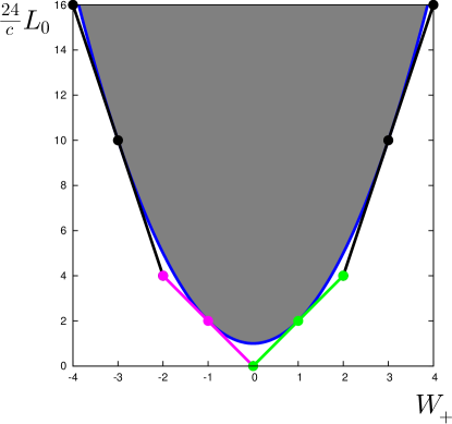
Figure 2: The plane of charges $(L_{0},W_{+})$ for the BTZ solutions with Wilson line (52). The green line corresponds to the chiral primaries. The lines in other colors are states from other sectors in the CFT, which can be mapped to the chiral primaries through spectral flow (i.e. states corresponding to geometries with $n\neq 0$ in (54). The parabola corresponds to the black hole threshold $M=J$, states under the parabola have $J>M$ (remember we chose $J>0$). Note that states of middle R-charge in their sector touch on the black hole threshold.

The upper bound on the R-charge is a result from superconformal field theory [42]. States violating this bound are forbidden by unitarity and, according to the AdS/CFT conjecture, cannot be part of the spectrum in a consistent quantum gravity theory on AdS₃. It is however not clear at all that such a bound can already be observed in the supergravity approximation. The AdS/CFT conjecture however suggests that in the full string theory this bound will be explictely imposed in the bulk, and for that reason the bound goes under the name of the stringy exclusion principle [25]. Further on we observe exactly this effect, by taking into account additional light brany degrees of freedom we see how the naive supergravity description gets corrected and how the stringy exclusion principle is explicitly realized directly in the bulk, without resorting to the AdS/CFT correspondence.

Finally, remember that by spectral flow a similar unitarity bound applies in the other sectors in the CFT as well. Table 1 provides an overview.

Sector	Boundary conds.	Quantum #s	Unitarity bounds
$n=0$	NS	$L_{0}={c\over 12}W{}_{+}$	$0\leq{R}\leq{c\over 6}$	$\Leftrightarrow$	$0\leq W{}_{+}\leq 2$
		${R}={c\over 12}W{}_{+}$
$n=1$	R	$L_{0}={c\over 24}$	$|{R}|\leq{c\over 12}$	$\Leftrightarrow$	$|W{}_{+}|\leq 1$
		${R}={c\over 12}W{}_{+}$
general $n$	$n$ even: NS	$L_{0}=\frac{c}{24}[-n(n-2)$	$-n\leq W{}_{+}\leq 2-n$
		$\quad\quad-2(n-1)W{}_{+}]$
	$n$ uneven: R	${R}=\frac{c}{12}W{}_{+}$

Table 1: Quantum numbers and the unitarity bounds following from supersymmetry in the left-moving sector of the CFT. For $n=0$, we have chiral primaries in the NS sector, for $n=1$ ground states in the R sector and for $n=2$, anti-chiral primaries in the NS sector.

4 A dynamical mechanism for excising closed timelike curves

In this section, we will propose a dynamical mechanism for the excision of the region in Gödel space that contains closed timelike curves. We begin by identifying BPS brane excitations in string theory that become light in a region of Gödel space. We assume that they condense at the critical radius where they become exactly massless, forming a supersymmetric domain wall consisting of branes smeared on this radius. We then show that this mechanism is consistent in supergravity by finding the precise solution on the outside of the domain wall that satisfies the Israel matching conditions. This will turn out to be a spinning supersymmetric BTZ solution of the type discussed in section 3.3. Our proposal is therefore also interesting from the point of view of the outside geometry, as it removes the CTC region of the spinning BTZ metric near its core, replacing it with a harmless patch of the Gödel universe.

One new feature of our example is that we will find a discrete family of branes that become light in Gödel, distinguished by their R-charge quantum number (i.e. their angular momentum on the internal sphere). By dialling this quantum number we obtain, after working out the construction outlined above, a family of spinning supersymmetric BTZ geometries on the outside that are glued to Gödel in a manner that removes all CTCs. One very interesting feature, which we take as strong evidence that our proposed excision mechanism is consistent, is that the family of BPS geometries obtained in this way reproduces precisely the unitarity bound on BPS states in the dual CFT, corresponding to the stringy exclusion principle. For example, in the case of the geometries corresponding to chiral primary states in the CFT, not only does our construction know about the lower bound on the conformal weight (which could have been anticipated from the results of [16]), but it also correctly reproduces the upper bound. As far as we know, this is the first time the stringy exclusion principle in AdS₃/CFT₂ is reproduced from physics in the bulk

4.1 Probing Gödel space with RQ particles

The first step in our proposal involves the identification of stringy degrees of freedom that become light in a region of Gödel space. In section 3.1, we showed that the Gödel solution arises as the backreacted solution corresponding to an RQ brane in the origin carrying $(\pi,\pi,0)$ Q-particle charge as well as R-charge. We look for probe branes that cancel the Q7-charge in the background so as to produce a space that is asymptotically AdS. To do this in a supersymmetric manner, we need to consider RQ particles carrying $(-\pi,-\pi,0)$. These branes have negative tension and their worldvolume action is minus the action for a $(\pi,\pi,0)$ particle. We furthermore allow them to carry an amount of R-charge which we call $b$. Let us now demonstrate that such RQ particles have the desired properties. The worldline action for such particles was discussed in section 2.2.3, where it was also shown to be supersymmetric. It is given by:

$$S={1\over 8\pi G}\left[(\mu-1)\left(\int T\sqrt{-g}-\int C\right)-2\pi b\left(\int\sqrt{-g}-\int A^{L}\right)\right]\,.$$ (61)

Let us now evaluate the worldline action in the Gödel background (45), choosing a static gauge with respect to the Gödel time $t$. One easily sees that such a particle experiences a flat potential, which is a consequence of the fact that these probe particles are mutually BPS with the brane that produces the background geometry. The effective mass of the particle is $r$-dependent and has a positive contribution from the R-charge part and a negative contribution from the Q7-part:

$$M_{eff}\sim b-{(\mu-1)\over 2\pi}T=b-(\mu-1){1+r^{2}\over 1-r^{2}}\,.$$ (62)

Hence we see that, for $b\geq\mu-1$ which we will assume from now on, these branes become tachyonic in the region

$$r^{2}>{b-(\mu-1)\over b+(\mu-1)}\,.$$ (63)

At the critical radius

$$r_{0}^{2}\equiv{b-(\mu-1)\over b+(\mu-1)}\,,$$ (64)

the probe particles become massless, and we expect such probes to form a condensate. We now explore the effects of such a condensate.

4.2 Consistency of excision

In a first approximation, we can view such a condensate as a thin shell, formed by the RQ-branes discussed above, smeared over the critical surface $r=r_{0}={b-(\mu-1)\over b+(\mu-1)}$ with some constant density $\rho$. The shell forms a domain wall separating a solid cylinder cut out of Gödel space on the inside, and a vacuum solution without Q-particle charge outside, see figure 3. The values of $\rho,b$ and the outside geometry are fixed by the requirement that the jump conditions on the various fields (i.e. the the Israel matching conditions) are satisfied for our particular sources on the wall. This construction will remove the CTCs if $r_{0}\leq 1/\sqrt{\mu}$.

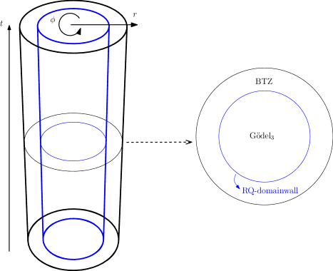
Figure 3: Here the global topology of the glued solution is depicted. Inside, i.e. for $0\leq r\leq r_{0}$, we have the Gödel solution. A domain wall of smeared RQ-particles interpolates between the outside vacuum geometry, which takes the form of a BTZ metric with specific mass and angular momentum.

4.2.1 The matched configuration

We show below that the matched configuration is completely specified by the total R-charge of the solution, or equivalently by the value of the Chern-Simons Wilson line at infinity which we will call $W_{+}$. Our matched solution is as follows.

On the inside, have the Gödel solution produced by a $(\pi,\pi,0)$ RQ particle at $r=0$ as discussed in section 3.2.2:

$$\frac{ds^{2}_{-}}{l^{2}} = -(dt+\mu\frac{r^{2}}{1-r^{2}}d\phi)^{2}+\mu\frac{dr^{2}+r^{2}d\phi^{2}}{(1-r^{2})^{2}}\,,$$ (65)

$$T_{-} = 2\pi{1+r^{2}\over 1-r^{2}}\,,$$ (66)

$$G_{-} = {8\pi lr\over(1-r^{2})^{2}}dr\wedge\left(dt+{\mu r^{2}\over(1-r^{2})}d\phi\right)\,,$$ (67)

$$A^{L}_{-} = W_{-}{l\over 2}d\phi\qquad W_{-}=1-\mu\,.$$ (68)

The radial variable runs from 0 to $r_{0}$, where we place a thin shell of $(-\pi,-\pi,0)$ particles with R-charge $b$, smeared with a constant density $\rho$. The values of these parameters are

$$r_{0}^{2} = {W_{+}\over 2(\mu-1)+W_{+}}\,,$$ (69)

$$b = W_{+}+\mu-1\,,$$ (70)

$$\rho = {1\over 2\pi}\,.$$ (71)

On the outside, we take a BTZ-type metric (52) for values of the radial coordinate $U\geq U_{0}$, with a Wilson line for $A^{L}$ turned on:

$$\frac{ds_{+}^{2}}{l^{2}} = -(d\tilde{t}+Ud\tilde{\phi})^{2}+\tilde{f}(U)d\tilde{\phi}^{2}+{dU^{2}\over 4\tilde{f}(U)}\,,$$ (72)

$$\tilde{f}(U) = U^{2}+\alpha U+{J\over 2}\,,$$ (73)

$$T_{+} = 2\pi{1+r_{0}^{2}\over 1-r_{0}^{2}}\,,$$ (74)

$$G_{+} = 0\,,$$ (75)

$$A^{L}_{+} = W_{+}{l\over 2}d\tilde{\phi}\,,$$ (76)

where, as before, $\alpha$ is defined by $J-M=\alpha^{2}$. The parameters in the outside solution are given by

$$\alpha = 1-W_{+}\,,$$ (77)

$$J = {\mu W_{+}^{2}\over 2(\mu-1)}\,,$$ (78)

$$M = J-(1-W_{+})^{2}\,,$$ (79)

$$U_{0} = {\mu W_{+}\over 2(\mu-1)}\,.$$ (80)

As a consistency check, it is easy to see that the metric of the complete solution is continuous. However, verifying whether the equations of motion are satisfied, by checking if indeed the jumps in the other fields and derivatives of the metric are exactly those produced by the domain wall source takes a little more work. We detail the calculation in the following subsection.

4.2.2 The Israel matching conditions

We now show that the above configuration satisfies the Israel matching conditions [44, 6], needed to ensure the glued solution satisfies the equations of motion also at the position of the delta-function sources. The Israel matching conditions follow from considering the bulk action (3) coupled to a domain wall action given by

$$S = {1\over 16\pi G}\int d^{3}x\left[{\cal L}_{bulk}+{\delta(r-r_{0})}{\cal L}_{DW}\right]$$ (81)

$${\cal L}_{bulk} = \sqrt{-g}\left(R+\frac{2}{l^{2}}-(\mu-1)\left({\partial_{\mu}T\partial^{\mu}T+{1\over 2}G_{\mu\nu}G^{\mu\nu}\over T^{2}-4\pi^{2}}\right)\right)-{2\over l}\epsilon^{\mu\nu\rho}A^{L}_{\mu}\partial_{\nu}A^{L}_{\rho}\,,$$ (82)

$${\cal L}_{DW} = {2\rho\over\sqrt{g_{rr}}}\left[((\mu-1)T-2\pi b)\sqrt{-g_{tt}}-(\mu-1)C_{t}+2\pi bA^{L}_{t}\right]\,.$$ (83)

We derive the solution presented in the previous subsection by explicitly showing how the parameters $(r_{0},b,\rho)$ and $(U_{0},J,M)$ are fixed to the values given above by the matching conditions.

The matching conditions require the metrics $ds^{2}_{\pm}$ to be continuous across the matching surface. This determines the parameters $U_{0},J$

$$U_{0} = {\mu r_{0}^{2}\over 1-r_{0}^{2}}\,,$$ (84)

$$J = {2\mu r_{0}^{2}\over(1-r_{0}^{2})^{2}}\left(1-\mu r_{0}^{2}-\alpha(1-r_{0}^{2})\right)\,.$$ (85)

We are now ready to solve the jump conditions on the fields across the shell. First of all, it is easy to see that the Bianchi identity $dG=0$ is obeyed everywhere without delta-function terms. This is because $G_{-}$ only has legs along the $r$-direction. Next, we note that the values of $\rho$ and $b$ are fixed by axionic and Chern-Simons charge conservation. Since the Gödel background has one unit of $(\pi,\pi,0)$ axionic charge and the axionic charge on the outside vanishes, the total $(-\pi,-\pi,0)$ charge on the wall also has to add up to one. This fixes $\rho$ to be

$$\rho={1\over 2\pi}\,,$$ (86)

Similarly, the total Chern-Simons charge on the wall is given by $2\pi\rho b=b$. On the outside we have charge $W_{+}$, while on the inside we have $W_{-}$, so $b$ is

$$b=W_{+}-W_{-}=W_{+}+\mu-1\,.$$ (87)

Plugging into (64) we find that the shell is located at

$$r_{0}^{2}={W_{+}\over 2(\mu-1)+W_{+}}\,.$$ (88)

Note that, for our embedding in string theory discussed in Appendix A, where $\mu=3/2$, $b$ becomes

$$b={1\over 2}+{R\over N^{2}}\,,$$ (89)

and is allowed by the quantization condition from string theory (152). In Appendix C, we show that these values for $\rho,b$ obtained by naive charge conservation indeed solve the precise Israël conditions for the fields $T,C$ and $A^{L}$.

Now we turn to the matching condition on the metric. Since our brane source is massless by construction, this amounts to requiring continuity of the extrinsic curvature across the matching surface:

$$K^{+}_{ij}=K^{-}_{ij}\,,$$ (90)

with

$$K_{ij}={1\over 2}{\cal L}_{n}h_{ij}\,,$$ (91)

where $n$ is the unit normal to the surface. The extrinsic curvatures are given by

$$K^{+}_{ij} = {l\sqrt{\mu}r_{0}\over(1-r_{0}^{2})}\left(\begin{array}[]{cc}0&-1\\ -1&\alpha\end{array}\right)\,,$$ (94)

$$K^{-}_{ij} = {l\sqrt{\mu}r_{0}\over(1-r_{0}^{2})}\left(\begin{array}[]{cc}0&-1\\ -1&{1-(2\mu-1)r_{0}^{2}\over 1-r_{0}^{2}}\end{array}\right)\,.$$ (97)

The gravitational matching equations (90) then require

$$\alpha = {1-{r_{0}^{2}\over r_{B}^{2}}\over 1-r_{0}^{2}}\,.$$ (99)

Here we have defined a special radius

$$r_{B}={1\over\sqrt{2\mu-1}}\,.$$ (100)

where $\alpha$ becomes zero and to which we will refer to as the ‘Bousso radius’ for reasons to be explained in section 4.2.5. Utilizing (88) we finally reproduced the complete solution as presented above.

4.2.3 Global supersymmetry

Let us now verify that our matched spacetime preserves half of the supersymmetries. The inside Gödel solution is half-BPS as shown in section 3.2.2. In section 3.3 we saw that, for NS sector boundary conditions on the fermions, the BTZ metric is supersymmetric if $\alpha$ is related to the Wilson line $W_{+}$ as

$$\alpha=1-W_{+}\,.$$ (101)

Plugging (88) into (99), we find that this is indeed precisely the relation obeyed by our outside geometry. We can also explicitly see that our matched solution preserves global Killing spinors. These were derived in (226) and (237) for the Gödel and BTZ geometries respectively and are given by

$$\epsilon_{+}=\epsilon_{-}=e^{-it}\epsilon_{0}\qquad{\rm with}\ \gamma_{\hat{\bar{z}}}\epsilon_{0}=0\,.$$ (102)

This establishes that our matched solution globally preserves half of the supersymmetries of (2,0) supergravity: it consists of two half-BPS solutions, glued across a thin shell in such a way that the Killing spinors are continuous, using matter on the shell that is separately supersymmetric.

Putting all this together we obtain the matched solution given in (68-80). It’s also useful to look at the quantum numbers of our glued space in the dual CFT:

$$L_{0} = {c\over 24}(M-J+1+W_{+}^{2})={c\over 12}W_{+}$$ (103)

$$R = {c\over 12}W_{+}$$ (104)

$$\bar{L}_{0} = {c\over 24}(M+J+1)={c\over 24}{W_{+}(W_{+}+2(\mu-1))\over\mu-1}$$ (105)

The first two equations are the characteristic quantum numbers of a chiral primary in the left-moving superconformal algebra. The third equation tells us that we have a particular excited state on the right-moving side. Of course, we could modify the value of $\bar{L}_{0}$ by adding rightmoving excitations of extra matter fields, present in the string embedding of our system, such as rightmoving Wilson lines.

Summarizing, we have found asymptotically AdS solutions corresponding to the backreaction of a solid cylinder of Gödel space with massless RQ particles smeared on the edge of the cylinder. In the dual CFT, the left moving quantum numbers are those of a chiral primary state of the (2,0) superconformal field theory while the rightmovers are in a specific non-supersymmetric excited state. We have obtained in this way a family of matched solutions that are characterized by the total R-charge and illustrated in Figure 4.

Figure 4: The family of matched solutions obtained. Left: position of the domain wall in Gödel. Middle: their dual CFT quantum numbers. Right: their mass and angular momentum. For zero R-charge (in orange), the Gödel region has zero size and we simply have global $AdS_{3}$. Increasing the R-charge progressively increases the size of the Gödel region. The Bousso radius (in blue) corresponds to the maximal entropy configuration on the black hole threshold. The maximal radius beyond which there would be CTCs (in red) corresponds to the maximum R-charge allowed by unitarity.

4.2.4 Chronology protection and stringy exclusion

Let’s discuss our matched solution (115) from the point of view of chronology protection. We found that our massless branes condense at radius

$$r_{0}^{2}={W_{+}\over 2(\mu-1)+W_{+}}\,.$$ (106)

We can vary the position $r_{0}$ of the domain wall by varying the R-charge of the matter on the wall, which will change the value of $W_{+}$. From the bulk gravity point of view, there are constraints on the value of $r_{0}$. The first requirement is that $r_{0}$ is positive; this simply leads to $W_{+}\geq 0$ or $L_{0}\geq 0$ as expected from [16]. A second constraint arises when one requires that the glued space is free of closed timelike curves. For this we should impose $r_{0}^{2}\leq 1/\mu$ which gives gives $W_{+}\leq 2$. One easily checks that this also implies that the outside metric is free of CTCs. These requirements agree precisely with the unitarity bounds on chiral primaries (60) in the dual CFT, the latter bound being the stringy exclusion principle (see Figure 4). Hence our construction gives a bulk gravity explanation for the stringy exclusion principle!

Of course one can also turn this argument around, and observe that if one imposes the unitarity bound of the dual CFT on the bulk solutions, that the remaining matched solutions are free of closed timelike curves. In this sense our result here is a generalization of the observation made in [16], that unitarity on the boundary seems equivalent to chronology protection in the bulk.

4.2.5 The extremal black hole limit

There is a special value of $W_{+}$, namely

$$W_{+}=1\,,$$ (107)

which is interesting both from the point of view of the inside as well as the outside geometry (see figure 4).

From the point of view of the Gödel space, the gluing radius becomes equal to what we called the Bousso radius:

$$r_{0}=r_{B}={1\over\sqrt{2\mu-1}}\,.$$ (108)

This radius is special in that it is the radius where the $\phi$ circle has maximum length. In Bousso’s proposal for holographic descriptions of general space-times [45], this is where the optimal holographic screen is located [46]. Therefore the worldvolume theory on our domain wall would be a candidate for a holographic dual description.

In this particular case, the outside metric has $M=J>0$ and lies at the extremal black hole threshold. As we can see from (51), the outside metric is really a scaling limit of the BTZ metric, controlled by the parameter $\alpha=\sqrt{J-M}\rightarrow 0$. In this limit, we approach extremality while we take a near-horizon limit and rescale energies at the same time. In this case, the outside metric can be written as

$$\frac{ds^{2}_{+}}{l^{2}}=-{2\over J}(U^{2}+{J\over 2})dt^{2}+{dU^{2}\over 4(U^{2}+{J\over 2})}+{J\over 2}(d\phi+{2U\over J}dt)^{2}\,.$$ (109)

Hence we obtain a circle fibration over $AdS_{2}$. This scaling limit goes under the name of the selfdual orbifold and was considered in [47] (see [48] for a recent discussion). The limit also corresponds to special quantum numbers in the dual CFT: the corresponding ensemble of BPS states has maximal degeneracy within the family of chiral primaries.

The degeneracy of chiral primaries has a symmetry around this middle value of the R-charge. As we can think of the chiral primaries as represented by harmonic forms, with their degree corresponding to the R-charge [25], Hodge duality then indeed provides a map between states of charge $R$ and those of charge $R_{\mathrm{max}}-R$. In our notation, as specified in table 1, this corresponds to $W_{+}\rightarrow 2-W_{+}$. It is interesting to note that this symmetry is reflected in the matched solutions we described above. If one computes the length of the circle on which the domain wall is smeared one finds:

$$L=2\pi l\sqrt{\frac{\mu}{4(\mu-1)}W_{+}(2-W_{+})}\,,$$ (110)

which is indeed invariant under this ’reflection of R-charge’. This is suggestive of a relation between the degeneracies of the chiral primaries and the area of the domain wall, it would be interesting to attempt a quantization of the domain wall and investigate what degeneracies one finds and how they relate to that of the chiral primaries in the theory.

4.2.6 Spectral flow

The solutions discussed above obey NS boundary conditions on the spinors. We can obtain configurations with different boundary conditions on the spinors by performing an integral spectral flow on the matched solution, which corresponds in the bulk to shifting both Wilson lines $W_{+},W_{-}$ with an integer number $n$. The resulting configuration is

$$J = {\mu(W_{+}+n)^{2}\over(2(\mu-1))}\,,$$ (111)

$$M = J-(1-n-W_{+})^{2}\,,$$ (112)

$$r_{0}^{2} = {W_{+}+n\over 2(\mu-1)+W_{+}+n}\,,$$ (113)

$$U_{0} = {\mu(W_{+}+n)\over 2(\mu-1)}\,,$$ (114)

$$b = W_{+}+\mu-1\,.$$ (115)

The preserved Killing spinors are then

$$\epsilon_{+}=\epsilon_{-}=e^{-it+i{n\over 2}\phi}\epsilon_{0}\qquad\mbox{with}\ \gamma_{\hat{\bar{z}}}\epsilon_{0}=0\qquad(\Leftrightarrow\gamma^{\hat{t}}\epsilon_{0}=i\epsilon_{0})\,.$$ (116)

A discussion similar to the one above gives the limits

$$-n\leq W_{+}\leq-n+2\,.$$ (117)

which again corresponds to the unitarity bounds in these sectors. For example, at $n=1$, the outside solutions are R sector ground states, and for $n=2$ we have antichiral primaries.

5 Conclusions and outlook

In this paper, we proposed a stringy mechanism for excising the closed timelike curves in the three-dimensional Gödel universe. We started by constructing explicit solutions arising from the backreaction of 7-branes wrapping an internal $S^{3}\times T^{4}$, and showed that these produce quotients of the Gödel metric. A special role was reserved for the brane with charges $(\pi,\pi,0)$ which produces the global Gödel metric accompanied by a Wilson line.

Next we studied probe branes in this background and identified certain branes that become light in some region of the space. We included these states in the effective description by assuming they condense on a thin shell at the radius where they become massless. We then found the geometry on the outside of the shell by solving the Israel matching conditions, and showed that the construction is supersymmetric. We found in this way a discrete one-parameter family of such glued configurations, labeled by their asymptotic R-charge as illustrated in figure 4. Our main observation was that demanding the absence of closed timelike curves in this family of solutions is equivalent to imposing the stringy exclusion bounds on chiral primaries in the dual CFT. We see this as evidence for the consistency of our proposal.

Our analysis has revealed some suggestive features that we feel deserve further study. One such feature is the apparent correspondence between the length of circle on which branes condense and the microscopic degeneracy of the outside configuration viewed as an ensemble in the dual CFT. In particular, the symmetry of the degeneracies appears to be correspond to a symmetry of the area under a reflection around the maximal area curve. The maximal length curve corresponds to to the location of Bousso’s optimal holographic screen, and the corresponding CFT quantum numbers are those of the maximal entropy configuration on the black threshold. These observations point to the possibility that the worldvolume theory of the matter on the shell would be a natural candidate for a holographic description of our glued spacetime. The model studied here could in this sense serve as a test case for understanding holography in more general non-asymptotically AdS spaces, such as Kerr-CFT [49], warped AdS backgrounds [50] or de Sitter space [51]. To make progress along these lines one would need a better understanding of the worldvolume degrees of freedom of our condensing branes. We saw that they have an internal angular momentum component and a generalized 7-brane component; it would be interesting to see if the thin shell we constructed can be seen as a type of giant graviton hypertube.

Finally, let us comment on the relation to [6], where supersymmetric Gödel embeddings were found in M-theory, corresponding to the backreaction of wrapped M2-branes. Treated as probes these M2 branes were shown to provide the correct degrees of freedom to describe the entropy of the D4D0 black hole [52]. One would now like to apply the new insights obtained in the present paper, namely how the addition of Q7-branes can resolve the closed timelike curves of the Gödel space, to that setup, by going through a chain of U-dualities [6]. It would be interesting to see if this could lead to a more precise description of the deconstruction model [52] that takes backreaction into account, and if the first hints we found concerning the degeneracies of chiral primaries and Gödel holography could be made more concrete in that setting.

Appendix A Type IIB embedding of (2,0) supergravity

In this appendix we show the reduction and consistent truncation that embeds (2,0)-supergravity (3) into Type IIB supergravity. We show this for the equations of motion, the generic 7-brane actions of [19] and the supersymmetry variations of the theory.

A.1 Type IIB conventions

We start from type IIB supergravity in the formalism of [53], truncated to include gravity, the selfdual five-form and the axion-dilaton. We define SL(2,$\mathbb{R}$)/SO(2) coset 1-forms ${{\cal P}},{\cal Q}$ given in terms of the standard axiodilaton $\tau$ as

$${{\cal P}} \equiv {d\tau\over\sqrt{2}\mathrm{Im}\,\tau}\,,$$ (118)

$${\cal Q} \equiv {1\over\mathrm{Im}\tau}d\mathrm{Re}\tau,.$$ (119)

They satisfy

$$d{\cal Q}=i{{\cal P}}\wedge\bar{{\cal P}}\,,$$ (120)

$$d{{\cal P}}+i{\cal Q}\wedge{{\cal P}}=0\,.$$ (121)

The (pseudo-) action is

$$S={2\pi\over l_{s}^{8}}\int_{{\cal M}_{10}}\left[\star R-{{\cal P}}\wedge\star\bar{{\cal P}}-{1\over 2\cdot 5!}F_{5}\wedge\star F_{5}\right]\,,$$ (122)

where, as usual, we have to impose the selfduality constraint $F_{5}=\star F_{5}$ at the level of the equations of motion.

The equations of motion are

$$R_{MN} = {1\over 2}({{\cal P}}_{M}\bar{{\cal P}}_{N}+{{\cal P}}_{N}\bar{{\cal P}}_{M})+{1\over 4\cdot 4!}F_{MPQRS}F_{N}^{\ PQRS}\,,$$ (123)

$$(\nabla^{M}+i{\cal Q}^{M}){{\cal P}}_{M} = 0\,,$$ (124)

$$F_{5} = \star F_{5}\,.$$ (125)

We will also consider Q7-brane sources [19, 20]. These couple to the supergravity fields as

$$S_{Q}={2\pi\over l_{s}^{8}}\left[-\int_{{\cal M}_{8}}T_{Q}\sqrt{-g}+\int_{{\cal M}_{8}}C_{8\,Q}\right]\,.$$ (126)

Here $Q$ is a traceless real matrix, parameterized by three charges, ($p,q,r$),

$$Q=\begin{pmatrix}\frac{r}{2}&p\\ -q&-\frac{r}{2}\end{pmatrix}\,.$$ (127)

The tension and the precise 8-form that the 7-brane couples to depend on $Q$:

$$T_{Q} = \frac{1}{\mathrm{Im}\,\tau}\left(p+r\mathrm{Re}\tau+q|\tau|^{2}\right)=2\sqrt{\det Q}\coth\left(\sqrt{\det Q}\mathrm{Im}\,\upsilon_{Q}\right)\,,$$ (128)

$$dC_{8\,Q} = \frac{\sqrt{\det Q}\star\!d\mathrm{Re}\,\upsilon_{Q}}{\sinh^{2}\left(\sqrt{\det Q}\mathrm{Im}\,\upsilon_{Q}\right)}\,.$$ (129)

The relation between $\tau$ and $\upsilon_{Q}$ is given by

$$\begin{cases}\tau=-\frac{r}{2q}-\frac{\sqrt{\det Q}}{q}\cot\left(\sqrt{\det Q}\,\upsilon_{Q}\right)\qquad\mbox{when }q>0\\ \tau=\frac{p}{r}\left(e^{r\upsilon_{Q}}-1\right)\ \ \,\quad\qquad\qquad\qquad\qquad\mbox{when }q=0\,.\end{cases}$$ (130)

A.2 Reduction ansatz

We are interested in compactifications of the above theory on $S^{3}\times T^{4}$, with Q7-brane sources wrapping on $S^{3}\times T^{4}$. For this, we take the following ansatz for the fields:

$$ds^{2} = ds^{2}_{3}+l^{2}d\tilde{\Omega}_{3}^{2}+V^{1\over 2}ds^{2}_{T^{4}}\,,$$ (131)

$$d\tilde{\Omega}_{3}^{2} = {1\over 4}\left[d\theta^{2}+\sin^{2}\theta d\psi_{R}^{2}+(D_{L}\psi_{L}+\cos\theta d\psi_{R})^{2}\right];\qquad D_{L}\psi_{L}\equiv d\psi_{L}+{4\over l}A^{L}\,,$$ (132)

$$F_{5} = {2\over l}(e^{0}\wedge e^{1}\wedge e^{2}+e^{3}\wedge e^{4}\wedge e^{5})\wedge S_{+}\,,$$ (133)

$$\tau = \tau(x^{a})\,,$$ (134)

where $x^{a}$ are the coordinates on the remaining 3d manifold, $ds^{2}_{4}$ is the unit volume flat metric on $T^{4}$ and $S_{+}$ is a closed, selfdual 2-form on $T^{4}$: $dS_{+}=0,\ S_{+}=\star_{4}S_{+}$. We have allowed a nontrivial fibration of the $S^{3}$ by a 3D gauge field $A$; this will give rise to a $U(1)$ Chern-Simons field in 3D. This $U(1)$ sits in the $SU(2)_{L}$ of the $SU(2)_{L}\times SU(2)_{R}$ of the sphere isometry group; by interchanging the $L$ and $R$ labels one gets a $U(1)$ in $SU(2)_{R}$. The Bianchi identity for $F_{5}$ requires that $F^{L}\equiv dA^{L}=0$.

In general we can decompose

$$S_{+}=n^{i}s_{i},\qquad n\cdot n=1\,,$$ (135)

with

$$s_{1} = {1\over\sqrt{2}}(e^{6}\wedge e^{7}+e^{8}\wedge e^{9})\,,$$ (136)

$$s_{2} = {1\over\sqrt{2}}(e^{6}\wedge e^{8}+e^{9}\wedge e^{7})\,,$$ (137)

$$s_{3} = {1\over\sqrt{2}}(e^{6}\wedge e^{9}+e^{7}\wedge e^{8})\,,$$ (138)

so that $\int_{T^{4}}S_{+}\wedge S_{+}=V$. The $S_{i}$ transform as a triplet under the $SU(2)_{L}$ subgroup of the $SO(4)$ frame rotations; we will later use this freedom to fix $n^{i}$ to a convenient value without loss of generality. Flux quantization tells us that the $F_{5}$ flux through any cycle should be an integer multiple of $l_{s}^{4}$; this gives the quantization condition

$$l^{2}={Nl_{s}^{4}\over 4\pi^{2}V^{1\over 2}}\,.$$ (139)

Verifying the equations of motion, one finds that the $S^{3}$ and $T^{4}$ parts are satisfied and one is left with the 3D equations

$$R_{ab}+{2\over l^{2}}g_{ab} = {{\cal P}}_{a}\bar{{\cal P}}_{b}+{{\cal P}}_{b}\bar{{\cal P}}_{a}\,,$$ (140)

$$(\nabla^{a}+i{\cal Q}^{a}){{\cal P}}_{a} = 0\,,$$ (141)

$$dF_{L} = 0\,.$$ (142)

These can be derived from an effective 3D action describing $AdS$ gravity coupled to an axion-dilaton system and a $U(1)$ Chern-Simons gauge field:

$$S={2\pi\over l_{3}}\int_{{\cal M}_{3}}\left[\star(R+{2\over l^{2}})-2{{\cal P}}\wedge\star\bar{{\cal P}}-{1\over l}A^{L}\wedge F^{L}\right]\,.$$ (143)

This is precisely the (2,0) action (3) with the parameter $\mu$ fixed to $\mu=3/2$. The three-dimensional Planck length is

$$l_{3}={l_{s}^{8}\over 2\pi^{2}l^{3}V}=32\pi^{2}G\,.$$ (144)

From these relations we find the Brown-Henneaux central charge:

$$c={3l\over 2G}={48\pi^{2}l\over l_{3}}=6N^{2}\,.$$ (145)

The U(1) Chern-Simons field is part of an SU(2)_L Chern-Simons field. Since $\pi_{3}(SU(2))=\mathbb{Z}$, the coefficient of the action is quantized in terms of the integer level $k$ In our normalization, the level is

$$k={8\pi^{2}l\over l_{3}}={c\over 6}=N^{2}\,,$$ (146)

which is indeed integer.

A.3 BPS source terms

Here we discuss how the 3d point particle actions discussed in section 2.2 follow from reduction.

First look at the 3D source terms produced by a Q7-brane wrapped on $S^{3}\times T^{4}$. Reducing (126) one finds

$$S_{Q}={1\over 16\pi G}\left[-\int T_{Q}ds+\int C_{Q}\right]\,.$$ (147)

We will also consider consider another BPS source, namely a BPS particle charged under $A$. Is this a KK mode on the three-sphere. Such source terms produce the BPS conical defects discussed in [35]. The action is

$$S_{CD}={b\over 4G}\left[-\int ds+\int A^{L}\right]\,,$$ (148)

where $b$ is the mass (= charge) of the particle.

Let’s find the quantization condition on $b$. In the dual CFT, the $U(1)_{L}$ R-charge $R$ is an integer. It corresponds to an asymptotic Wilson line going as

$$A^{L}={R\over k}ld\phi\,.$$ (149)

The field strength has a delta-singularity:

$$F^{L}={R\over k}l\delta(r)dr\wedge d\phi\,.$$ (150)

This in turn is produced by a source term

$${R\over l}\int A^{L}\,.$$ (151)

Hence $b$ is quantized as

$$b={R\over k}={R\over N^{2}}\,.$$ (152)

A.4 Spinor reduction

We now discuss the reduction ansatz for the spinors. We will first reduce to six dimensions and then use the results of [35] to further reduce to 3D. The type IIB Killing spinor equations coming from the gravitino and dilatino variations are

$$\left(\nabla_{M}-{i\over 4}{\cal Q}_{M}+{i\over 8\cdot 4!}F_{MNPQR}\Gamma^{NPQR}\right)\epsilon_{10} = 0$$ (153)

$$\Gamma^{M}{{\cal P}}_{M}\epsilon^{c}_{10} = 0\,.$$ (154)

Here, $\epsilon_{10}$ is a 10D Weyl spinor

$$\Gamma_{11}\epsilon_{10}=\epsilon_{10},\qquad\Gamma_{11}\equiv\Gamma^{0}\Gamma^{1}\ldots\Gamma^{9}$$ (155)

and conjugation is defined as

$$\epsilon^{c}_{10}=(B_{10}\epsilon_{10})^{*},\qquad B_{10}\Gamma^{M}B_{10}^{-1}=\Gamma^{M*},\ B_{10}^{*}B_{10}=1\,.$$ (156)

Using these properties, the complex conjugates of (154) are equivalent to

$$\left(\nabla_{M}+{i\over 2}{\cal Q}_{M}-{i\over 8\cdot 4!}F_{MNPQR}\Gamma^{NPQR}\right)\epsilon_{10}^{c} = 0\,,$$ (157)

$$\Gamma^{M}\bar{{\cal P}}_{M}\epsilon_{10} = 0\,.$$ (158)

We decompose the gamma-matrices according into $SO(1,5)\times SO(4)\subset SO(1,9)$

$$\Gamma^{\mu} = \tilde{\gamma}^{\mu}\otimes\gamma_{(5)}\qquad\mu=0,\ldots,5$$ (159)

$$\Gamma^{i} = 1\otimes\gamma^{i}\qquad i=6,\ldots,9$$ (160)

$$\Gamma_{(11)} = \gamma_{(7)}\otimes\gamma_{(5)}$$ (161)

$$B_{10} = B_{6}\otimes B_{4}$$ (162)

$$\gamma_{(7)} = \tilde{\gamma}^{0}\tilde{\gamma}^{1}\ldots\tilde{\gamma}^{5}\qquad\gamma_{(5)}=\gamma^{6}\gamma^{7}\gamma^{8}\gamma^{9}$$ (163)

$$B_{6}\tilde{\gamma}^{\mu}B_{6}^{-1} = \tilde{\gamma}^{\mu*},\qquad B_{6}^{*}B_{6}=-1$$ (164)

$$B_{4}\gamma^{i}B_{4}^{-1} = \gamma^{i*},\qquad B_{4}^{*}B_{4}=-1\,.$$ (165)

Now we expand in a special basis of $SO(4)$ spinors. Because the Weyl spinor representation of $SO(4)$ is pseudoreal, we can find basis spinors $\eta^{\pm}_{A},\ A=1,2$ that satisfy

$$\gamma_{(5)}\eta^{\pm}_{A} = \pm\eta^{\pm}_{A}\,,$$ (166)

$$(B_{4}\eta^{\pm}_{A})^{*} = \epsilon^{AB}\eta^{\pm}_{B}\qquad\epsilon^{12}\equiv 1\,.$$ (167)

We now decompose the 10D spinors $\epsilon_{10},\ \epsilon_{10}^{c}$ into 6D spinors $\Psi^{\pm}_{l},\ l=1,\ldots,4$ according to the ansatz

$$\epsilon_{10} = \Psi^{+}_{1}\otimes\eta^{+}_{1}+\Psi^{+}_{4}\otimes\eta^{+}_{2}+\Psi^{-}_{1}\otimes\eta^{-}_{1}+\Psi^{-}_{4}\otimes\eta^{-}_{2}\,,$$ (168)

$$\epsilon_{10}^{c} = \Psi^{+}_{2}\otimes\eta^{+}_{1}+\Psi^{+}_{3}\otimes\eta^{+}_{2}+\Psi^{-}_{2}\otimes\eta^{-}_{1}+\Psi^{-}_{3}\otimes\eta^{-}_{2}\,.$$ (169)

The 10D chirality and reality condition (156) reduce to conditions on the 6D spinors:

$$\gamma_{(7)}\Psi^{\pm}_{m} = \pm\Psi^{\pm}_{m}\qquad m=1,\ldots,4\,,$$ (170)

$$(B_{6}\Psi^{\pm}_{m})^{*} = \Omega_{m}^{\ n}\Psi^{\pm}_{n}\,,$$ (171)

where

$$\Omega_{m}^{\ n}=\left(\begin{array}[]{cccc}0&0&1&0\\ 0&0&0&1\\ -1&0&0&0\\ 0&-1&0&0\end{array}\right)\,.$$ (172)

The second condition is the symplectic Majorana condition, so we have decomposed the 10D spinor into two 6D symplectic Majorana-Weyl spinors of opposite chirality.

Now we can plug our spinor decomposition ansatz (169) into the Killing spinor equations (154) using the reduction ansatz (134). Let’s start with the $T^{4}$ components of the gravitino equation. These reduce to

$$(1+\gamma_{(7)}\otimes 1)\epsilon_{10}=0\,,$$ (173)

or, in terms of the 6D spinors:

$$\Psi^{+}_{m}=0\,.$$ (174)

so we are left with a single symplectic Majorana-Weyl spinor $\Psi^{-}_{m}$.

Now we write out the susy conditions on the 6D spinor $\Psi^{-}_{m}$. We define the 6D selfdual 3-form $H$ as

$$H_{3}={1\over l}(e^{0}\wedge e^{1}\wedge e^{2}+e^{3}\wedge e^{4}\wedge e^{5})\qquad*_{6}H_{3}=H_{3}\,.$$ (175)

The operator $S_{+ij}\gamma^{ij}$ generates an $SU(2)_{L}\subset SO(4)$ rotation under which the $\eta^{-}_{A}$ transform as a doublet and the $\eta^{+}_{A}$ as a singlet. By choosing a suitable frame on $T^{4}$ we can arrange that

$${1\over 2}S_{+ij}\gamma^{ij}\eta^{-}_{A}=i\sigma^{3\ B}_{A}\eta^{-}_{B}.$$ (176)

Then the 6D part of the KS equations (154,158) reduces to

$$\left(\nabla_{\mu}-{i\over 2}{\cal Q}_{\mu}-{1\over 4}H_{\mu\nu\rho}\tilde{\gamma}^{\nu\rho}\right)\Psi^{-}_{1} = 0\,,$$ (177)

$$\left(\nabla_{\mu}+{i\over 2}{\cal Q}_{\mu}+{1\over 4}H_{\mu\nu\rho}\tilde{\gamma}^{\nu\rho}\right)\Psi^{-}_{2} = 0\,,$$ (178)

$$\left(\nabla_{\mu}+{i\over 2}{\cal Q}_{\mu}-{1\over 4}H_{\mu\nu\rho}\tilde{\gamma}^{\nu\rho}\right)\Psi^{-}_{3} = 0\,,$$ (179)

$$\left(\nabla_{\mu}-{i\over 2}{\cal Q}_{\mu}+{1\over 4}H_{\mu\nu\rho}\tilde{\gamma}^{\nu\rho}\right)\Psi^{-}_{4} = 0\,,$$ (180)

$$\gamma^{\mu}{{\cal P}}_{\mu}\Psi^{-}_{1} = 0\,,$$ (181)

$$\gamma^{\mu}\bar{{\cal P}}_{\mu}\Psi^{-}_{2} = 0\,,$$ (182)

$$\gamma^{\mu}\bar{{\cal P}}_{\mu}\Psi^{-}_{3} = 0\,,$$ (183)

$$\gamma^{\mu}{{\cal P}}_{\mu}\Psi^{-}_{4} = 0\,.$$ (184)

For ${{\cal P}}={\cal Q}=0$, we recover precisely the equations (40) in [35]. Although we wont do this explicitly, let us point out that these eqs. should be embeddable in 6d N =4b supergravity with tensor multiplets.

Next we reduce to 3D using the conventions of [35]. We decompose the Clifford matrices as

$$\tilde{\gamma}^{\alpha} = \sigma_{1}\otimes 1\otimes\gamma^{\alpha}\qquad\alpha=0,1,2\,,$$ (185)

$$\tilde{\gamma}^{a} = \sigma_{2}\otimes\gamma^{a}\otimes 1\qquad a=3,4,5\,,$$ (186)

$$\gamma^{0} = -i\sigma_{2}\qquad\gamma^{1}=\sigma_{1}\qquad\gamma^{2}=\sigma_{3}\,,$$ (187)

$$\gamma^{3} = \sigma_{1}\qquad\gamma^{4}=\sigma_{2}\qquad\gamma^{5}=\sigma_{3}\,,$$ (188)

$$\gamma_{(7)} = \sigma_{3}\otimes 1\otimes 1\,,$$ (189)

$$B_{6} = \gamma^{3}\gamma^{5}=1\otimes-i\sigma_{2}\otimes 1\,.$$ (190)

The only difference with the conventions of [35] is that we have chosen another $B_{6}$. We will need the useful identities

$$\gamma^{\alpha\beta} = \epsilon^{\alpha\beta\delta}\gamma_{\delta}\,,$$ (191)

$$\gamma^{ab} = i\epsilon^{abc}\gamma_{c}\,.$$ (192)

The chirality condition means that we can write

$$\Psi^{-}_{m}=\left(\begin{array}[]{c}0\\ 1\end{array}\right)\otimes\varepsilon_{l}\,,$$ (193)

with $\varepsilon_{l}$ 4-component spinors. Now we work out the $S^{3}$ part of the gravitino equation. For this it is convenient to choose the left-invariant vielbein:

$$e^{3} = {l\over 2}(\cos\psi_{L}d\theta+\sin\psi_{L}\sin\theta d\psi_{R})\,,$$ (194)

$$e^{4} = {l\over 2}(-\sin\psi_{L}d\theta+\cos\psi_{L}\sin\theta d\psi_{R})\,,$$ (195)

$$e^{5} = {l\over 2}(D_{L}\psi_{L}+\cos\theta d\psi_{R})\,.$$ (196)

The spin connection is

$$\omega_{34} = -{1\over l}(e^{5}-2A^{L})\,,$$ (197)

$$\omega_{53} = -{1\over l}e^{4}\,,$$ (198)

$$\omega_{45} = -{1\over l}e^{3}\,.$$ (199)

If we take the Killing spinor to be independent of the $S^{3}$ coordinates, the $S^{3}$ gravitino equation projects

$$\varepsilon_{1}=\varepsilon_{3}=0.$$ (200)

The remaining 3D equations for $\varepsilon_{2,4}$ are

$$\left(\partial_{\alpha}+{1\over 4}\omega_{\alpha}^{\hat{\beta}\hat{\gamma}}\epsilon_{\hat{\beta}\hat{\gamma}\hat{\delta}}1\otimes\gamma^{\hat{\delta}}-{1\over 2l}e_{\alpha}^{\hat{\alpha}}1\otimes\gamma_{\hat{\alpha}}+{i\over l}A^{L}_{\alpha}\sigma_{3}\otimes 1+{i\over 4}{\cal Q}_{\alpha}\right)\varepsilon_{2} = 0\,,$$ (201)

$$\left(\partial_{\alpha}+{1\over 4}\omega_{\alpha}^{\hat{\beta}\hat{\gamma}}\epsilon_{\hat{\beta}\hat{\gamma}\hat{\delta}}1\otimes\gamma^{\hat{\delta}}-{1\over 2l}e_{\alpha}^{\hat{\alpha}}1\otimes\gamma_{\hat{\alpha}}+{i\over l}A^{L}_{\alpha}\sigma_{3}\otimes 1-{i\over 4}{\cal Q}_{\alpha}\right)\varepsilon_{4} = 0\,,$$ (202)

$$\bar{{\cal P}}_{\alpha}1\otimes\gamma^{\alpha}\varepsilon_{2}\ = 0\,,$$ (203)

$${{\cal P}}_{\alpha}1\otimes\gamma^{\alpha}\varepsilon_{4}\ = 0\,,$$ (204)

while the reality condition (171) imposes

$$(i\sigma_{2}\otimes 1)\varepsilon_{2}^{*}=\varepsilon_{4}\,.$$ (205)

We can now embed the Izquierdo-Townsend solutions [31]. Suppose we have a 2-component spinor $\epsilon$ solving the equations (5):

$$\left(\partial_{\alpha}+{1\over 4}\omega_{\alpha}^{\hat{\beta}\hat{\gamma}}\epsilon_{\hat{\beta}\hat{\gamma}\hat{\delta}}\gamma^{\hat{\delta}}-{1\over 2l}e_{\alpha}^{\hat{\alpha}}\gamma_{\hat{\alpha}}-{i\over l}A^{L}_{\alpha}-{i\over 4}{\cal Q}_{\alpha}\right)\epsilon = 0\,,$$ (206)

$${{\cal P}}_{\alpha}\gamma^{\alpha}\epsilon\ = 0\,.$$ (207)

Then we can solve (204) by embedding it as

$$\varepsilon_{4}=\left(\begin{array}[]{c}0\\ \epsilon\end{array}\right)\qquad\varepsilon_{2}=\left(\begin{array}[]{c}-\epsilon^{*}\\ 0\end{array}\right)\,.$$ (208)

If the background has ${{\cal P}}={\cal Q}=0$, the number of 10D supersymmetries is doubled, because there is then a second embedding

$$\varepsilon_{4}=\left(\begin{array}[]{c}\epsilon^{*}\\ 0\end{array}\right)\qquad\varepsilon_{2}=\left(\begin{array}[]{c}0\\ \epsilon\end{array}\right)\,.$$ (209)

Similarly if $A^{L}=0$ there is a second embedding

$$\varepsilon_{4}=\left(\begin{array}[]{c}\epsilon\\ 0\end{array}\right)\qquad\varepsilon_{2}=\left(\begin{array}[]{c}0\\ \epsilon^{*}\end{array}\right)\,.$$ (210)

As explained in [35], there is a further doubling of 10d supersymmetries if there is also a right moving Wilson line $A^{R}$ turned on with $A^{R}=A^{L}$. Then by using a right-invariant vielbein on $S^{3}$ we can find additional embeddings as above with $\varepsilon_{4}$ replaced by $\varepsilon_{1}$ and $\varepsilon_{2}$ by $\varepsilon_{3}$. In this way, the maximally susy $AdS_{3}$ vacuum of (2,0) supergravity lifts to a IIB solution preserving 16 supersymmetries, while the half-BPS Gödel and conical defect solutions of (2,0) supergravity lift to solutions preserving 8 supersymmetries.

Appendix B Supersymmetry details

We discuss two supersymmetric solutions to the (2,0) supergravity system (3): one where the metric is of BTZ-type and the axidilaton is constant, and another where the axidilaton is holomorphic and the metric is Gödel space. In both cases we allow a Wilson line for the CS gauge field.

B.1 BPS equations and notation

We repeat the Killing spinor equations (5) for convenience:

$$\left(\partial_{\alpha}+B^{L}_{\alpha\hat{\beta}}\gamma^{\hat{\beta}}-{i\over l}A^{L}_{\alpha}-{i\over 2}(\mu-1)\;^{*}{\cal Q}_{\alpha}\right)\epsilon = 0\,,$$ (211)

$$(\mu-1)\;^{*}{{\cal P}}_{\alpha}\gamma^{\alpha}\epsilon\ = 0\,.$$ (212)

with the left gravitational Chern-Simons connection $B^{L}$:

$$B^{L}_{\alpha\hat{\beta}}={1\over 4}\omega_{\alpha}^{\ \hat{\gamma}\hat{\delta}}\epsilon_{\hat{\gamma}\hat{\delta}\hat{\beta}}-{1\over 2l}e_{\alpha\hat{\beta}}\,.$$ (213)

Both the BTZ and the Gödel metric can be written as a time fibration over Euclidean AdS₂. It will simplify the analysis if we choose a vielbein adapted to this fact. Both geometries can be written as

$$ds^{2}=-(e^{\hat{t}})^{2}+e^{\hat{z}}e^{\hat{\bar{z}}}\,.$$ (214)

We make use of a vielbein of the form:

$$e^{\hat{t}} = l(dt+{\chi})\,,$$

$${}e^{\hat{z}} = le^{\varphi}dz\,,$$

$${}e^{\bar{\hat{z}}} = le^{\varphi}d\bar{z}\,.$$ (215)

For the case we consider, the vielbein furthermore obeys the properties:

$$de^{\hat{t}} = \frac{i}{l}e^{\hat{z}}\wedge e^{\hat{\bar{z}}}\,,$$ (216)

$$de^{\hat{z}} = -{2i\over l\nu}(e^{\hat{t}}-ld\Lambda)\wedge e^{\hat{z}}\,,$$ (217)

where $\nu$ is a constant and $d\Lambda$ a closed one-form on the full three dimensional spacetime. Using these properties we can compute the spin connection

$$\omega^{\hat{t}\hat{z}} = -{i\over l}e^{\hat{z}}\,,$$

$${}\omega^{\hat{z}\hat{\bar{z}}} = -\frac{2i}{\nu l}\left((\nu-2)e^{\hat{t}}+2ld\Lambda\right)\,,$$ (218)

and the connection $B^{L}_{\alpha\hat{\beta}}$:

$$B^{L}\equiv B^{L}_{\alpha\hat{\beta}}dx^{a}\otimes e^{\hat{\beta}}=\frac{1}{l\nu}\left((\nu-1)e^{\hat{t}}+ld\Lambda\right)\otimes e^{\hat{t}}\,.$$ (219)

B.2 Supersymmetry for global Gödel solution

Our (2,0) supergravity model also has a solution where the axidilaton is holomorphic and the spacetime is globally Gödel. The global Gödel solution corresponds to

$$\det Q=\pi^{2}.$$ (220)

and has the following metric, scalars and Wilson line:

$$ds^{2} = -(dt+{\chi})^{2}+e^{2\varphi}dzd\bar{z}\,,$$

$${}A^{L} = \frac{l}{2}(\mu-1)d\arg z\,,$$

$${}\tau = i\frac{1+z}{1-z}\,,$$ (221)

with

$${\chi}=\mu\frac{|z|^{2}}{1-|z|^{2}}d\arg z\,,\qquad e^{2\varphi}=\frac{\mu}{(1-|z|^{2})^{2}}\,.$$ (222)

Because of holomorphy of $\tau$, the dilatino equation becomes a projection condition

$$\gamma_{\hat{\bar{z}}}\epsilon=0\qquad(\Leftrightarrow\gamma^{\hat{t}}\epsilon=i\epsilon).$$ (223)

One easily checks the vielbein choice (215) satisfies the properties (217) with

$$\nu = \mu$$

$${}\Lambda = t.$$ (224)

The relevant quantities entering in the covariant derivative are (see (10))

$$B_{L} = (dt+{\mu-1\over\mu}{\chi})\otimes e^{\hat{t}}$$

$${}A^{L} = (1-\mu){l\over 2}d\arg z$$

$${}{\cal Q} = d\arg z+{2\over\mu}{\chi}$$ (225)

Note that, using the spinor projection condition (223), the nontrivial holonomies nicely cancel between the different connections. The Killing spinor equations are solved by

$$\epsilon=e^{-it}\epsilon_{0}\qquad\text{with}\ \gamma_{\hat{\bar{z}}}\epsilon_{0}=0\qquad(\Leftrightarrow\gamma^{\hat{t}}\epsilon_{0}=i\epsilon_{0}).$$ (226)

We conclude that the three-dimensional solution 221 is a 1/2 BPS to (2,0) supergravity.

B.3 Supersymmetry for BTZ type solution

We start from the BTZ type metric in the form (52) used for the matching of the field equations, with Wilson line $A^{L}$ also given in (52). First, we rewrite the metric (52), with spatial coordinates $U,\tilde{\phi}$ in terms of the complex coordinate

$$z=\rho e^{i\tilde{\phi}}\,,$$ (227)

where $\rho=|z|$ is related to the radial coordinate $U$ as

$$d\ln\rho=\frac{dU}{2\tilde{f}(U)}\,.$$ (228)

The metric is then given as:

$$\frac{ds^{2}}{l^{2}} = \left(-(dt+{\chi})^{2}+e^{2\varphi}dzd\bar{z}\right)\,,$$ (229)

where ${\chi}$ and $\varphi$ read in terms of $z$:

$${\chi} = Ud\arg z\,,$$

$${}e^{2\varphi} = \frac{\tilde{f}(U)}{|z|^{2}}\,,$$ (230)

and $U$ is to be seen as a function of $|z|$ through (228).

It is straightforward to check that the choice of vielbein (215) satisfies the conditions (216,217), with

$$\nu = 1\,,$$ (231)

$$\Lambda = t+\frac{1-\alpha}{2}\arg z\,.$$ (232)

The gauge connections entering in the spinor covariant derivative are:

$$B_{L} = (dt+{1-\alpha\over 2}d\phi)\otimes e^{\hat{t}}\,,$$ (233)

$$A^{L} = \frac{l}{2}W_{+}d\arg z\,,$$ (234)

Since the complex scalar $\tau=cst$ in this solution, only the gravitino equation is non-trivial. It reads:

$$\left(\partial_{\alpha}+(\partial_{\alpha}t)\gamma^{\hat{t}}+\frac{1}{2}\partial_{\alpha}(\arg z)\big{(}(1-\alpha)\gamma^{\hat{t}}-iW_{+}\big{)}\right)\epsilon=0\,.$$ (235)

We search for spinors with projection condition $\gamma^{\hat{t}}\epsilon=i\epsilon$ as in the Gödel solution, eq. (226). In order for the spinors to obey sensible boundary conditions (periodic or anti-periodic in $\phi$), we require

$$W_{+}=1-\alpha-n\,,\qquad n\in\mathbb{Z}\,.$$ (236)

The solution for the Killing spinor equation then reads:

$$\epsilon=e^{-it-i\frac{n}{2}\phi}\epsilon_{0}\,,\qquad\text{with}\quad\gamma_{\hat{\bar{z}}}\epsilon_{0}=0\qquad(\Leftrightarrow\gamma^{\hat{t}}\epsilon_{0}=i\epsilon_{0})\,.$$ (237)

Hence the BTZ-type solution with Chern-Simons Wilson line obeying (236) is a half BPS solution.

Note that the Killing spinors (237) of the BTZ spaces match to those of the Gödel solution (226) only when $n=0$. This corresponds to having NS boundary conditions for the spinors. When $n\neq 0$, we can shift $W_{+}\rightarrow W_{+}-n$ in order to preserve the Gödel Killing spinor. This corresponds to performing a spectral flow in the dual CFT from another sector back to the NS sector.

Appendix C Matching conditions for the non-gravitational fields

In the main text we fixed the constants $\rho$ and $b$ by a quick argument based on charge conservation. Here we show that this physical intuition is correct and that these solutions solve the equations of motion in the presence of the domain wall. Thinking of the domain wall as a $\delta$-function source there should be jumps present in the radial dependence of the fields to cancel this term in the equations of motion. More precisely, the equations of motion at the position of the domain wall take the form:

$$\Delta I=j$$ (238)

with $\Delta f=f_{+}-f_{-}$. Taking $n$ to be a unit normal vector to the matching surface, and assuming a two derivative bulk action for the field $\phi$ these expressions become

$$I=n_{\mu}\frac{\delta{\cal L}_{\mathrm{bulk}}}{\delta\partial_{\mu}\phi}\qquad\mbox{and}\qquad j=\frac{\delta{\cal L}_{\mathrm{DW}}}{\delta\phi}$$ (239)

Using the Lagrangian (81) in the case of our interest we can compute

$$I_{T} = n_{\mu}{\delta{\cal L}_{bulk}\over\delta(\partial_{\mu}T)}=-2(\mu-1)\sqrt{-g}{n^{\mu}\partial_{\mu}T\over T^{2}-4\pi^{2}}\,,$$ (240)

$$I_{C}^{i} = n_{\mu}{\delta{\cal L}_{bulk}\over\delta\partial_{\mu}C_{i}}=-2(\mu-1)\sqrt{-g}{n_{\mu}G^{\mu i}\over T^{2}-4\pi^{2}}\,,$$ (241)

$$I_{A^{L}}^{i} = 2n_{\mu}{\delta{\cal L}_{bulk}\over\delta\partial_{\mu}{A^{L}}_{i}}=-{4\over l}n_{\mu}\epsilon^{\mu ij}{A^{L}}_{j}\,.$$ (242)

The factor 2 in the last line arises because because the CS-Lagrangian is first order in derivatives and hence both the $A^{L}$ variation and the $\partial_{\mu}{A^{L}}$ variation of the bulk action give rise to a delta-function term with equal coefficient. For the unit normal we concretely take

$$n_{+}={1\over\sqrt{g_{UU}}}\partial_{U}\,,\qquad\qquad n_{-}={1\over\sqrt{g_{rr}}}\partial_{r}\,.$$ (243)

The source terms from the domain wall are

$$j_{T} = {\delta{\cal L}_{DW}\over\delta T}=2l(\mu-1)\rho\,,$$ (244)

$$j^{i}_{C} = {\delta{\cal L}_{DW}\over\delta C_{i}}=2(\mu-1)\rho\delta^{i}_{t}\,,$$ (245)

$$j^{i}_{A^{L}} = {\delta{\cal L}_{DW}\over\delta{A^{L}}_{i}}=-4\pi\rho b\delta^{i}_{t}\,.$$ (246)

Computing the inside ($-$) and outside ($+$) values for the $I$’s, and the explicit form of the $j$’s from (68) and (76) we can see that the matching equations (238) are satisfied for each of the fields. So we see that this more detailed analysis reproduces the result obtained by the argument based on charge conservation.

References

- [1] K. Godel, An Example of a new type of cosmological solutions of Einstein’s field equations of graviation, Rev. Mod. Phys. 21 (1949) 447–450.
- [2] M. Rooman and P. Spindel, Goedel metric as a squashed anti-de Sitter geometry, Class. Quant. Grav. 15 (1998) 3241–3249, [gr-qc/9804027].
- [3] S. W. Hawking and G. F. R. Ellis, The Large scale structure of space-time, . Cambridge University Press, Cambridge, 1973.
- [4] J. P. Gauntlett, J. B. Gutowski, C. M. Hull, S. Pakis, and H. S. Reall, All supersymmetric solutions of minimal supergravity in five dimensions, Class. Quant. Grav. 20 (2003) 4587–4634, [hep-th/0209114].
- [5] D. Israel, Quantization of heterotic strings in a Goedel/anti de Sitter spacetime and chronology protection, JHEP 01 (2004) 042, [hep-th/0310158].
- [6] T. S. Levi, J. Raeymaekers, D. Van den Bleeken, W. Van Herck, and B. Vercnocke, Godel space from wrapped M2-branes, JHEP 01 (2010) 082, [arXiv:0909.4081].
- [7] J. L. Friedman and A. Higuchi, Topological censorship and chronology protection, Annalen Phys. 15 (2006) 109–128, [arXiv:0801.0735].
- [8] S. W. Hawking, The Chronology protection conjecture, Phys. Rev. D46 (1992) 603–611.
- [9] B. S. Kay, M. J. Radzikowski, and R. M. Wald, Quantum field theory on spacetimes with a compactly generated Cauchy horizon, Commun. Math. Phys. 183 (1997) 533–556, [gr-qc/9603012].
- [10] J. M. Maldacena, The large n limit of superconformal field theories and supergravity, Adv. Theor. Math. Phys. 2 (1998) 231–252, [hep-th/9711200].
- [11] L. Susskind and E. Witten, The holographic bound in anti-de Sitter space, hep-th/9805114.
- [12] C. A. R. Herdeiro, Special properties of five dimensional BPS rotating black holes, Nucl. Phys. B582 (2000) 363–392, [hep-th/0003063].
- [13] M. M. Caldarelli, D. Klemm, and W. A. Sabra, Causality violation and naked time machines in AdS(5), JHEP 05 (2001) 014, [hep-th/0103133].
- [14] M. M. Caldarelli, D. Klemm, and P. J. Silva, Chronology protection in anti-de Sitter, Class. Quant. Grav. 22 (2005) 3461–3466, [hep-th/0411203].
- [15] A. Dabholkar, N. Iizuka, A. Iqubal, and M. Shigemori, Precision microstate counting of small black rings, Phys. Rev. Lett. 96 (2006) 071601, [hep-th/0511120].
- [16] J. Raeymaekers, D. Van den Bleeken, and B. Vercnocke, Relating chronology protection and unitarity through holography, JHEP 1004 (2010) 021, [arXiv:0911.3893].
- [17] M. Banados, C. Teitelboim, and J. Zanelli, The Black hole in three-dimensional space-time, Phys. Rev. Lett. 69 (1992) 1849–1851, [hep-th/9204099].
- [18] M. Banados, M. Henneaux, C. Teitelboim, and J. Zanelli, Geometry of the (2+1) black hole, Phys. Rev. D48 (1993) 1506–1525, [gr-qc/9302012].
- [19] E. A. Bergshoeff, J. Hartong, T. Ortin, and D. Roest, Seven-branes and supersymmetry, JHEP 02 (2007) 003, [hep-th/0612072].
- [20] E. Bergshoeff, J. Hartong, and D. Sorokin, Q7-branes and their coupling to IIB supergravity, JHEP 12 (2007) 079, [arXiv:0708.2287].
- [21] M. Banados, G. Barnich, G. Compere, and A. Gomberoff, Three dimensional origin of Goedel spacetimes and black holes, Phys. Rev. D73 (2006) 044006, [hep-th/0512105].
- [22] C. V. Johnson, A. W. Peet, and J. Polchinski, Gauge theory and the excision of repulson singularities, Phys. Rev. D61 (2000) 086001, [hep-th/9911161].
- [23] N. Drukker, B. Fiol, and J. Simon, Goedel’s universe in a supertube shroud, Phys. Rev. Lett. 91 (2003) 231601, [hep-th/0306057].
- [24] E. G. Gimon and P. Horava, Over-rotating black holes, Goedel holography and the hypertube, hep-th/0405019.
- [25] J. M. Maldacena and A. Strominger, Ads(3) black holes and a stringy exclusion principle, JHEP 12 (1998) 005, [hep-th/9804085].
- [26] J. de Boer, S. El-Showk, I. Messamah, and D. V. d. Bleeken, A bound on the entropy of supergravity?, arXiv:0906.0011.
- [27] A. Achucarro and P. K. Townsend, A Chern-Simons Action for Three-Dimensional anti-De Sitter Supergravity Theories, Phys. Lett. B180 (1986) 89.
- [28] E. Witten, (2+1)-Dimensional Gravity as an Exactly Soluble System, Nucl. Phys. B311 (1988) 46.
- [29] A. Achucarro and P. K. Townsend, Extended supergravities in d=(2+1) as Chern-Simons theories, Phys. Lett. B229 (1989) 383.
- [30] J. R. David, Anti-de Sitter gravity associated with the supergroup SU(1,1—2) x SU(1,1—2), Mod. Phys. Lett. A14 (1999) 1143–1148, [hep-th/9904068].
- [31] J. M. Izquierdo and P. K. Townsend, Supersymmetric space-times in (2+1) adS supergravity models, Class. Quant. Grav. 12 (1995) 895–924, [gr-qc/9501018].
- [32] S. Deser, R. Jackiw, and G. ’t Hooft, Three-Dimensional Einstein Gravity: Dynamics of Flat Space, Ann. Phys. 152 (1984) 220.
- [33] S. Deser and R. Jackiw, Three-Dimensional Cosmological Gravity: Dynamics of Constant Curvature, Annals Phys. 153 (1984) 405–416.
- [34] J. R. David, G. Mandal, S. Vaidya, and S. R. Wadia, Point mass geometries, spectral flow and AdS(3)-CFT(2) correspondence, Nucl. Phys. B564 (2000) 128–141, [hep-th/9906112].
- [35] V. Balasubramanian, J. de Boer, E. Keski-Vakkuri, and S. F. Ross, Supersymmetric conical defects: Towards a string theoretic description of black hole formation, Phys. Rev. D64 (2001) 064011, [hep-th/0011217].
- [36] J. M. Maldacena and L. Maoz, De-singularization by rotation, JHEP 12 (2002) 055, [hep-th/0012025].
- [37] A. Sen, F-theory and Orientifolds, Nucl. Phys. B475 (1996) 562–578, [hep-th/9605150].
- [38] E. A. Bergshoeff, M. de Roo, S. F. Kerstan, and F. Riccioni, IIB supergravity revisited, JHEP 0508 (2005) 098, [hep-th/0506013].
- [39] P. Kraus and F. Larsen, Partition functions and elliptic genera from supergravity, JHEP 01 (2007) 002, [hep-th/0607138].
- [40] V. Balasubramanian and P. Kraus, A stress tensor for anti-de Sitter gravity, Commun. Math. Phys. 208 (1999) 413–428, [hep-th/9902121].
- [41] J. D. Brown and M. Henneaux, Central Charges in the Canonical Realization of Asymptotic Symmetries: An Example from Three-Dimensional Gravity, Commun. Math. Phys. 104 (1986) 207–226.
- [42] W. Lerche, C. Vafa, and N. P. Warner, Chiral Rings in N=2 Superconformal Theories, Nucl. Phys. B324 (1989) 427.
- [43] J. McGreevy, L. Susskind, and N. Toumbas, Invasion of the giant gravitons from anti-de Sitter space, JHEP 06 (2000) 008, [hep-th/0003075].
- [44] W. Israel, Singular hypersurfaces and thin shells in general relativity, Nuovo Cim. B44S10 (1966) 1.
- [45] R. Bousso, Holography in general space-times, JHEP 06 (1999) 028, [hep-th/9906022].
- [46] E. K. Boyda, S. Ganguli, P. Horava, and U. Varadarajan, Holographic protection of chronology in universes of the Goedel type, Phys. Rev. D67 (2003) 106003, [hep-th/0212087].
- [47] O. Coussaert and M. Henneaux, Self-dual solutions of 2+1 Einstein gravity with a negative cosmological constant, hep-th/9407181.
- [48] V. Balasubramanian, J. Parsons, and S. F. Ross, States of a chiral 2d CFT, arXiv:1011.1803.
- [49] M. Guica, T. Hartman, W. Song, and A. Strominger, The Kerr/CFT Correspondence, arXiv:0809.4266.
- [50] D. Anninos, W. Li, M. Padi, W. Song, and A. Strominger, Warped Black Holes, JHEP 03 (2009) 130, [arXiv:0807.3040].
- [51] A. Strominger, The dS/CFT correspondence, JHEP 10 (2001) 034, [hep-th/0106113].
- [52] F. Denef, D. Gaiotto, A. Strominger, D. Van den Bleeken, and X. Yin, Black hole deconstruction, hep-th/0703252.
- [53] J. H. Schwarz, Covariant Field Equations of Chiral N=2 D=10 Supergravity, Nucl. Phys. B226 (1983) 269.