Delay-Based Back-Pressure Scheduling in Multihop Wireless Networks

Abstract

Scheduling is a critical and challenging resource allocation mechanism for multihop wireless networks. It is well known that scheduling schemes that favor links with larger queue length can achieve high throughput performance. However, these queue-length-based schemes could potentially suffer from large (even infinite) packet delays due to the well-known last packet problem, whereby packets belonging to some flows may be excessively delayed due to lack of subsequent packet arrivals. Delay-based schemes have the potential to resolve this last packet problem by scheduling the link based on the delay the packet has encountered. However, characterizing throughput-optimality of these delay-based schemes has largely been an open problem in multihop wireless networks (except in limited cases where the traffic is single-hop.) In this paper, we investigate delay-based scheduling schemes for multihop traffic scenarios with fixed routes. We develop a scheduling scheme based on a new delay metric, and show that the proposed scheme achieves optimal throughput performance. Further, we conduct simulations to support our analytical results, and show that the delay-based scheduler successfully removes excessive packet delays, while it achieves the same throughput region as the queue-length-based scheme.

I Introduction

Link scheduling is a critical resource allocation component in multihop wireless networks, and also perhaps the most challenging. The seminal work of [1] introduces a joint adaptive routing and scheduling algorithm, called Queue-length-based Back-Pressure (Q-BP), that has been shown to be throughput-optimal, i.e., it can stabilize the network under any feasible load. This paper focuses on the settings with fixed routes, where the Q-BP algorithm becomes a scheduling algorithm. Since the development of Q-BP, there have been numerous extensions that have integrated it in an overall optimal cross-layer framework. Further, easier-to-implement queue-length-based scheduling schemes have been developed and shown to be throughput-efficient (see [2] and references therein). Some recent attempts [3, 4, 5] focus on designing real-world wireless protocols using the ideas behind these algorithms.

While these queue-length-based schedulers have been shown to achieve excellent throughput performance, they are usually evaluated under the assumption that flows have an infinite amount of data and keep injecting packets into the network. However, in practice, when accounting for multiple time scales [6, 7, 8], there also exist other types of flows that have a finite number of packets to transmit, which can result in the well-known last packet problem: consider a queue that holds the last packet of a flow, then the packet does not see any subsequent packet arrivals, and thus the queue length remains very small and the link may be starved for a long time, since the queue-length-based schemes give a higher priority to links with a larger queue length. In such a scenario with flow-level dynamics, it has also been shown in [6] that the queue-length-based schemes may not even be throughput-optimal.

Recent works in [9, 10, 11, 12, 13, 14] have studied the performance of delay-based scheduling algorithms that use Head-of-Line (HOL) delays instead of queue lengths as link weights. One desirable property of the delay-based approach is that they provide an intuitive way around the last packet problem. The schedulers give a higher priority to the links with a larger weight as before, but now the weight (i.e., the HOL delay) of a link increases with time until the link is scheduled. Hence, if the link with the last packet is not scheduled at this moment, it is more likely to be scheduled in the next time. However, the throughput of the delay-based scheduling schemes is not fully understood, and has only been established for limited cases with single-hop traffic.

The delay-based approach was introduced in [9] for scheduling in Input-Queued switches. The results have been extended to wireless networks for single-hop traffic, providing throughput-optimal delay-based MaxWeight scheduling algorithms [11, 12, 15]. It has also been shown that delay-based schemes with appropriately chosen weight parameters provide good Quality of Service (QoS) [10], and can be used as an important component in a cross-layer protocol design [14]. The performance of the delay-based MaxWeight scheduler has been further investigated in a single-hop network with flow-level dynamics [13]. The results show that, when flows arrive at the base station carrying a finite amount of data, the delay-based MaxWeight scheduler achieves optimal throughput performance while its queue-length-based counterpart does not.

It should be noted that even for the multihop wireless networks with fixed routes, the scheduling problem is both important and challenging. There are many existing works focusing on such scenarios with fixed routes (see [16, 17, 18] for examples). However, in multihop wireless networks, the throughput performance of these delay-based schemes has largely been an open problem. To the best of our knowledge, even with the assumption of fixed routes, there are no prior works that employ delay-based algorithms to address the important issue of throughput-optimal scheduling in multihop wireless networks. Indeed, the problem becomes much more challenging in the multihop scenario. In [12], the key idea in showing throughput-optimality of the delay-based MaxWeight scheduler is to exploit the following property: after a finite time, there exists a linear relation between queue lengths and HOL delays in the fluid limits (which we formally define in Section III-A), where the ratio is the mean arrival rate. Hence, the delay-based MaxWeight scheme is basically equivalent to its queue-length-based counterpart, and thus achieves the optimal throughput. This property holds for the single-hop traffic. Since given that the exogenous arrival processes follow the Strong Law of Large Numbers (SLLN) and the fluid limits exist, the arrival processes are deterministic with constant rates in the fluid limits. However, such a linear relation does not necessarily hold for the multihop traffic, since at a non-source (or relay) node, the arrival process may not satisfy SLLN and the packet arrival rate may not even be a constant, depending on the underlying scheduler s dynamics. To this end, we investigate delay-based scheduling schemes that achieve optimal throughput performance in multihop wireless networks.

Unlike previous delay-based schemes, we view the packet delay as a sojourn time in the network, and re-design the delay metric of the queue as the sojourn-time difference between the queue’s HOL packet and the HOL packet of its previous hop (see Eq. (38) for the formal definition). Using this new metric, we can establish a linear relation between queue lengths and delays in the fluid limits. The linear relation then plays the key role in showing that the proposed Delay-based Back-Pressure (D-BP) scheduling scheme is throughput-optimal in multihop networks.

In summary, the main contributions of our paper are as follows:

• We devise a new delay metric for multihop wireless networks and develop the D-BP algorithm, under which a linear relation between queue lengths and delays in the fluid limits can be established. From this linear relation, we can show that D-BP achieves optimal throughput performance. To do this, we first re-visit throughput-optimality of Q-BP using fluid limit techniques. Further, we develop a simpler greedy approximation of D-BP for practical implementation.

• We provide extensive simulation results to evaluate the performance of the delay-based schedulers, including D-BP. Through simulations, i) we observe that the last packet problem can cause excessive delays for certain flows under Q-BP, while the problem is eliminated under D-BP. ii) We show that D-BP also achieves better fairness and prevents the flows that lack subsequent packet arrivals from starving. iii) Finally, we simulate the simpler greedy approximation algorithms of Q-BP and D-BP, and show that the delay-based approximation empirically achieves a throughput region that is no smaller than that of its queue-based counterpart.

The paper is organized as follows. In Section II, we present a detailed description of our system model. In Section III, we show throughput-optimality of Q-BP using fluid limit techniques, and extend the analysis to D-BP in Section IV. The discussions are further extended to the greedy algorithms in Section V. We evaluate the performance of delay-based schedulers through simulations in Section VI, and conclude our paper in Section VII.

II System Model

We consider a multihop wireless network described by a directed graph $\mathcal{G}=(\mathcal{V},\mathcal{E})$, where $\mathcal{V}$ denotes the set of nodes and $\mathcal{E}$ denotes the set of links. Nodes are wireless transmitters/receivers and links are wireless channels between two nodes if they can directly communicate with each other. During a single time slot, multiple links that do not interfere with each other can be active at the same time, and each active link transmits one packet during the time slot if its queue is not empty. Let $\mathcal{S}$ denote the set of flows in the network. We assume that each flow has a single, fixed, and loop-free route. The route of flow $s$ has an ${H}(s)$-hop length from the source to the destination, where each $k$-th hop link is denoted by $({s,k})$. Let ${H}^{\max}\triangleq\max_{s\in\mathcal{S}}{H}(s)<\infty$ denote the length of the longest route over all flows. Note that the assumption of single route and unit link capacity is only for ease of exposition, and one can readily extend the results to more general scenarios with multiple fixed routes and heterogeneous link rates, applying the techniques used in this paper. To specify wireless interference, we consider the $k$-th hop of each flow $s$ or link-flow-pair $({s,k})$. Let $\mathcal{P}$ denote the set of all link-flow-pairs, i.e.,

$$\mathcal{P}\triangleq\{({s,k})~{}|~{}s\in\mathcal{S},~{}1\leq k\leq{H}(s)\}.$$

The set of link-flow-pairs that interfere with $({s,k})$ can be described as

$$\begin{split}I({s,k})\triangleq\{({r,j})\in\mathcal{P}~{}|~{}&({r,j})~{}\text{interferes with}~{}({s,k}),\\ &\text{or}~{}({r,j})=({s,k})\}.\end{split}$$ (1)

Note that the interference model we adopt is very general, and includes the class of the $K$-hop interference model. A schedule is a set of (active or inactive) link-flow-pairs, and can be represented by a vector $\vec{M}\in\{0,1\}^{|\mathcal{P}|}$, where $|\cdot|$ denotes the cardinality of a set. Each element $M_{{s,k}}$ is set to 1 if link-flow-pair $({s,k})$ is active, and 0 if link-flow-pair $({s,k})$ is inactive. Slightly abusing the notation, we also use $M$ to denote the set of active link-flow-pairs of $\vec{M}$, i.e., $M\triangleq\{({s,k})\in\mathcal{P}~{}|~{}M_{s,k}=1\}$. A schedule $\vec{M}$ is said to be feasible if no two link-flow-pairs of $\vec{M}$ interfere with each other, i.e., $({r,j})\notin I({s,k})$ for all $({r,j})$, $({s,k})$ with $M_{r,j}=1$ and $M_{s,k}=1$. Let $\mathcal{M}_{\mathcal{P}}$ denote the set of all feasible schedules in $\mathcal{P}$, and let $Co(\mathcal{M}_{\mathcal{P}})$ denote its convex hull.

Let $A_{s}(t)$ denote the number of packet arrivals at the source node of flow $s$ at time slot $t$. We assume that packets are of unit length. Similar to [12], we assume that each arrival process $A_{s}(t)$ is a stationary and ergodic Markov chain with countable state space, and satisfies the Strong Law of Large Numbers (SLLN): That is, with probability one,

$$\textstyle\lim_{t\rightarrow\infty}\frac{\sum^{t-1}_{\tau=0}A_{s}(\tau)}{t}=\lambda_{s},$$ (2)

for each flow $s\in\mathcal{S}$, where $\lambda_{s}$ denotes the mean arrival rate of flow $s$. We let $\vec{\lambda}\triangleq[\lambda_{1},\lambda_{2},\cdots,\lambda_{|\mathcal{S}|}]$ denote the arrival rate vector.

Let $Q_{s,k}(t)$ denote the number of packets at the queue of $({s,k})$ at the beginning of time slot $t$. For notational ease, we also use $Q_{s,k}$ to denote the queue itself. We let $\vec{Q}(t)\triangleq[Q_{s,k}(t),~{}({s,k})\in\mathcal{P}]$ denote the queue length vector at time slot $t$, and use $\|\cdot\|$ to denote the $L_{1}$-norm of a vector, e.g., $\|\vec{Q}(t)\|=\sum_{({s,k})\in\mathcal{P}}Q_{s,k}(t)$. Let $\Pi_{s,k}(t)$ denote the service of $Q_{s,k}$ at time slot $t$, which takes a value of either 1 if link-flow-pair $({s,k})$ is active, or 0 otherwise, in our settings. We let $\Psi_{s,k}(t)$ denote the actual number of packets transmitted from $Q_{s,k}$ at time slot $t$. Clearly, we have $\Psi_{s,k}(t)\leq\Pi_{s,k}(t)$ for all time slots $t\geq 0$. Let $P_{s,k}(t)\triangleq\sum_{i=1}^{k}Q_{s,i}(t)$ denote the cumulative queue lengths up to the $k$-th hop for flow $s$. By convention, we set $Q_{s,{H}(s)+1}(t)=0$, and then we have $P_{s,{H}(s)+1}(t)=P_{s,{H}(s)}(t)$. The queue length evolves according to the following equations:

$$Q_{s,k}(t+1)=Q_{s,k}(t)+\Psi_{s,k-1}(t)-\Psi_{s,k}(t),$$ (3)

where we set $\Psi_{s,0}(t)=A_{s}(t)$.

Let $F_{s}(t)$ be the total number of packets that arrive at the source node of flow $s$ until time slot $t\geq 0$, including those present at time slot 0, and let $\hat{F}_{{s,k}}(t)$ be the total number of packets that are served at $Q_{{s,k}}$ until time slot $t\geq 0$. By convention, we set $\hat{F}_{{s,k}}(0)=0$ for all link-flow-pairs $({s,k})\in\mathcal{P}$. We let $Z_{{s,k},i}(t)$ denote the sojourn time of the $i$-th packet of $Q_{{s,k}}$ in the network at time slot $t$, where the time is measured from the time when the packet arrives in the network (i.e., when the packet arrives at the source node), and let $W_{{s,k}}(t)=Z_{{s,k},1}(t)$ denote the sojourn time of the HOL packet of $Q_{{s,k}}$ in the network at time slot $t$. We set $W_{s,0}(t)=0$ for all $s\in\mathcal{S}$. Further, if $Q_{s,k}(t)=0$, we set $W_{{s,k}}(t)=W_{s,k-1}(t)$. Letting $U_{s,k}(t)\triangleq t-W_{s,k}(t)$ denote the time when the HOL packet of $Q_{s,k}$ arrives in the network, we have that

$$U_{{s,k}}(t)=\inf\{\tau\leq t~{}|~{}F_{s}(\tau)>\hat{F}_{s,k}(t)\},~{}\text{for all}~{}t\geq 0.$$ (4)

As in [27], a discrete-time queueing system is said to be stable, if the underlying Markov chain is positive Harris recurrent. When the state space is countable and all states communicate (as in the system that we consider in this paper), this is equivalent to the Markov chain being positive recurrent. The throughput region of a scheduling policy is defined as the set of arrival rate vectors for which the network remains stable under this policy. Further, the optimal throughput region (or stability region) is defined as the union of the throughput regions of all possible scheduling policies. We let $\Lambda^{*}$ denote the optimal throughput region, which can be represented as

$$\Lambda^{*}\triangleq\{\vec{\lambda}~{}|~{}\exists\vec{\phi}\in Co(\mathcal{M}_{\mathcal{P}})~{}\text{s.t.}~{}\lambda_{s}\leq\phi_{s,k},\forall({s,k})\in\mathcal{P}\}.$$ (5)

An arrival rate vector is strictly inside $\Lambda^{*}$, if the inequalities above are all strict.

We summarize the notations in Appendix A for quick reference.

III Queue-length-based Back-Pressure Algorithm

It has been shown in [1] that Q-BP stabilizes the network for any feasible arrival rate vector using stochastic Lyapunov techniques. Specifically, we can use a quadratic Lyapunov function to show that the function has a negative drift under Q-BP when queue lengths are large enough. In this section, we re-visit throughput-optimality of Q-BP using fluid limit techniques. The analysis will be extended later to prove throughput-optimality of the delay-based back-pressure algorithm.

To begin with, we define the queue differential $\Delta Q_{s,k}(t)$ as

$$\Delta Q_{s,k}(t)\triangleq Q_{s,k}(t)-Q_{s,k+1}(t),$$ (6)

and specify the back-pressure algorithm based on queue lengths as follows.

Queue-length-based Back-Pressure (Q-BP) algorithm:

$$\textstyle\vec{M}^{*}\in\operatornamewithlimits{argmax}_{\vec{M}\in\mathcal{M}_{\mathcal{P}}}\sum_{({s,k})\in\mathcal{P}}\Delta Q_{s,k}(t)\cdot M_{s,k}.$$ (7)

The algorithm needs to solve a MaxWeight problem with weights as queue differentials, and ties can be broken arbitrarily if there is more than one schedule that has the largest weight sum.

We establish the fluid limits of the system in the following subsection.

III-A Fluid Limits

We define the process describing the behavior of the underlying system as $\mathcal{X}=(\mathcal{X}(t),t=0,1,2,\cdots)$, where

$$\mathcal{X}(t)\triangleq\left((Z_{{s,k},1}(t),\cdots,Z_{{s,k},Q_{{s,k}}(t)}(t)),({s,k})\in\mathcal{P}\right).$$

We define the norm of $\mathcal{X}(t)$ as

$$\|\mathcal{X}(t)\|\triangleq\|\vec{Q}(t)\|+\|\vec{W}(t)\|.$$ (8)

Clearly, under Q-BP, the evolution of $\mathcal{X}$ forms a discrete-time Markov chain with countable state space. Let $\mathcal{X}^{(x)}$ denote a process $\mathcal{X}$ with an initial configuration such that

$$\|\mathcal{X}^{(x)}(0)\|=x.$$ (9)

The following Lemma was derived in [28] for continuous-time countable Markov chains, and it follows from more general results in [29] for discrete-time countable Markov chains.

Lemma 1 (Theorem 4 of [12])

Suppose there exist an $\epsilon>0$ and a finite integer $T>0$ such that for any sequence of processes $\{\frac{1}{x}\mathcal{X}^{(x)}(xT),x=1,2,\cdots\}$, we have

$$\textstyle\limsup_{x\rightarrow\infty}\mathbf{E}\left[\frac{1}{x}\|\mathcal{X}^{(x)}(xT)\|\right]\leq 1-\epsilon.$$ (10)

Then, the Markov process $\mathcal{X}$ is positive recurrent.

A stability criteria of (10) leads to a fluid limit approach [30, 31] to the stability problem of queueing systems. Hence, we start our analysis by establishing the fluid limit model as in [30, 12]. We define the process $\mathcal{Y}\triangleq\left(A,F,\hat{F},Q,P,\Pi,\Psi,W,U\right)$, and it is clear that a sample path of $\mathcal{Y}^{(x)}$ uniquely defines the sample path of $\mathcal{X}^{(x)}$. Then we extend the definition of $Y=A,F,\hat{F},Q,P,\Pi,\Psi,W$ and $U$ to continuous time domain as $Y(t)\triangleq Y(\lfloor t\rfloor)$ for each continuous time $t\geq 0$.

As in [12], we extend the definition of $F^{(x)}_{s}(t)$ to the negative interval $t\in[-x,0)$ by assuming that the packets present in the initial state $\mathcal{X}^{(x)}(0)$ arrived in the past at some of the time instants $-(x-1),-(x-2),\cdots,0$, according to their delays in the state $\mathcal{X}^{(x)}(0)$. By this convention, we have $F^{(x)}_{s}(-x)=0$ for all $s\in\mathcal{S}$ and $x$, and $\sum_{s\in S}F^{(x)}_{s}(0)\leq x$ for all $x$.

Then, applying the techniques used in the proof for Theorem 4.1 of [30] or Lemma 1 of [12], we can show that with probability one, for any sequence of processes $\{\frac{1}{{x_{n}}}\mathcal{Y}^{({x_{n}})}({x_{n}}\cdot)\}$, where $\{{x_{n}}\}$ is a sequence of positive integers with ${x_{n}}\rightarrow\infty$, there exists a subsequence $\{{x_{n_{j}}}\}$ with ${x_{n_{j}}}\rightarrow\infty$ as $j\rightarrow\infty$ such that the following convergences hold uniformly over compact (u.o.c.) intervals:

$$\textstyle\frac{1}{{x_{n_{j}}}}\int_{0}^{{x_{n_{j}}}t}A^{({x_{n_{j}}})}_{s}(\tau)d\tau\rightarrow\lambda_{s}t,$$ (11)

$$\textstyle\frac{1}{{x_{n_{j}}}}F^{({x_{n_{j}}})}_{s}({x_{n_{j}}}t)\rightarrow f_{s}(t),$$ (12)

$$\textstyle\frac{1}{{x_{n_{j}}}}\hat{F}^{({x_{n_{j}}})}_{s,k}({x_{n_{j}}}t)\rightarrow\hat{f}_{s,k}(t),$$ (13)

$$\textstyle\frac{1}{{x_{n_{j}}}}Q^{({x_{n_{j}}})}_{s,k}({x_{n_{j}}}t)\rightarrow q_{s,k}(t),$$ (14)

$$\textstyle\frac{1}{{x_{n_{j}}}}P^{({x_{n_{j}}})}_{s,k}({x_{n_{j}}}t)\rightarrow p_{s,k}(t),$$ (15)

$$\textstyle\frac{1}{{x_{n_{j}}}}\int_{0}^{{x_{n_{j}}}t}\Pi^{({x_{n_{j}}})}_{s,k}(\tau)d\tau\rightarrow\int_{0}^{t}\pi_{s,k}(\tau)d\tau,$$ (16)

$$\textstyle\frac{1}{{x_{n_{j}}}}\int_{0}^{{x_{n_{j}}}t}\Psi^{({x_{n_{j}}})}_{s,k}(\tau)d\tau\rightarrow\int_{0}^{t}\psi_{s,k}(\tau)d\tau.$$ (17)

Similarly, the following convergences (which are denoted by “$\Rightarrow$”) hold at every continuous point of the limit function:

$$\textstyle\frac{1}{{x_{n_{j}}}}W^{({x_{n_{j}}})}_{s,k}({x_{n_{j}}}t)\Rightarrow w_{{s,k}}(t),$$ (18)

$$\textstyle\frac{1}{{x_{n_{j}}}}U^{({x_{n_{j}}})}_{s,k}({x_{n_{j}}}t)\Rightarrow u_{{s,k}}(t).$$ (19)

The above convergence properties follow directly from the Arzela-Ascoli Theorem and the structure of the model: that the arrival process satisfies the SLLN and that the sequence of the (scaled) departure process is uniformly bounded and uniformly equicontinuous.

Any set of limiting functions $(f,\hat{f},q,p,\pi,\psi,w,u)$ is called a fluid limit. The family of these fluid limits is associated with our original stochastic network. The scaled sequences $\{\frac{1}{{x_{n}}}\mathcal{Y}^{({x_{n}})}({x_{n}}\cdot)\}$ and their limits are referred to as a fluid limit model [27]. Since some of the limiting functions, namely $f_{s},\hat{f}_{s,k},q_{s,k},p_{s,k}$ are Lipschitz continuous in $[0,\infty)$, they are absolutely continuous. Hence, at almost all points $t\in[0,\infty)$, the derivatives of these limiting functions exist. We call such points regular time.

We then present the fluid model equations of the system as follows.

$$\textstyle\sum_{s\in\mathcal{S}}f_{s}(0)\leq 1,$$ (20)

$$\textstyle p_{s,k}(t)=\sum_{i=1}^{k}q_{s,i}(t),$$ (21)

$$\textstyle p_{s,k}(t)=f_{s}(t)-\hat{f}_{s,k}(t),$$ (22)

$$\textstyle f_{s}(t)=f_{s}(0)+\lambda_{s}t,$$ (23)

$$\textstyle u_{{s,k}}(t)=t-w_{{s,k}}(t),$$ (24)

$$\textstyle\psi_{s,k}(t)\leq\pi_{s,k}(t),$$ (25)

$$\textstyle\Delta q_{s,k}(t)=q_{s,k}(t)-q_{s,k+1}(t),$$ (26)

$$\textstyle\frac{d}{dt}q_{s,k}(t)=\left\{\begin{array}[]{ll}\psi_{s,k-1}(t)-\pi_{s,k}(t),&\text{if}~{}q_{s,k}(t)>0,\\ (\psi_{s,k-1}(t)-\pi_{s,k}(t))^{+},&\text{otherwise},\end{array}\right.$$ (29)

where $(z)^{+}\triangleq\max(z,0)$, and we set $\psi_{s,0}=\pi_{s,0}=\lambda_{s}$. Fluid model equations can be thought of as belonging to a fluid network which is the deterministic equivalence of the original stochastic network. Any set of functions satisfying the fluid model equations is called a fluid model solution of the system. It is easy to check that any fluid limit is a fluid model solution.

It is clear from (7) that Q-BP will not schedule link-flow-pair $({s,k})$ if $Q_{s,k}(t)-Q_{s,k+1}(t)<0$. Hence, if link-flow-pair $({s,k})$ is scheduled, it must satisfy that $Q_{s,k}(t)-Q_{s,k+1}(t)\geq 0$. Moreover, the length of queue $Q_{s,k}$ can decrease by at most one within one time slot, and the length of queue $Q_{s,k+1}$ can increase by at most one within one time slot, due to the assumption of unit link capacity (a similar argument also holds with non-unit link rates). This implies that, if

$$Q_{s,k}(t)\geq Q_{s,k+1}(t)-2$$ (30)

initially holds for all $({s,k})$ at time slot 0, then the inequality holds for every time slot $t\geq 0$. This further implies that

$$\ q_{s,k}(t)\geq q_{s,k+1}(t),~{}\text{i.e.},~{}\Delta q_{s,k}(t)\geq 0,$$ (31)

for all (scaled) time $t\geq 0$, from the convergence of (14). We assume that at time slot 0, all queues on the route of each flow are empty except for the first queue, then it follows that (30) holds for all (scaled) time $t\geq 0$, and thus, $\Delta q_{s,k}(t)\geq 0$ holds for all time $t\geq 0$.

 

Remark: Note that we make the assumption of empty queues for ease of analysis. Even without this assumption, we can show that there exists a finite time $T>0$ such that for all time $t\geq T$, (31) holds for all $({s,k})\in\mathcal{P}$. This can be proved by induction. The detailed proof can be found in Appendix C, but the basic idea is as follows: Consider a flow $\hat{s}\in\mathcal{S}$. We want to show that there exists a finite time $T_{\hat{s}}>0$ such that for all time $t\geq T_{\hat{s}}$, (31) holds for all $(\hat{s},k)$ with $k\in\{1,2,\cdots,{H}(\hat{s})\}$.

1. First, we show that there exists a finite time $T_{\hat{s},1}>0$ such that for all time $t\geq T_{\hat{s},1}$, (31) holds for link-flow-pair $(\hat{s},1)$. Suppose that (31) does not hold for $(\hat{s},1)$. Then Q-BP does not schedule $(\hat{s},1)$, i.e., $q_{\hat{s},1}(t)$ does not decrease and $q_{\hat{s},2}(t)$ does not increase. On the other hand, due to the exogenous arrivals at the source node of flow $\hat{s}$, $q_{\hat{s},1}(t)$ must increase with time. Hence, there must exist a finite time $T_{\hat{s},1}$ such that (31) holds for $(\hat{s},1)$ at time $T_{\hat{s},1}$. We can further show that (31) holds for all $t\geq T_{\hat{s},1}$ under Q-BP. This can be proved by contradiction.

2. Then, we discuss the induction step: Consider $k\in\{1,2,\cdots,{H}(\hat{s})-1\}$. Suppose that for all time $t\geq T_{\hat{s},k}>0$, (31) holds for $(\hat{s},j)$ and for all $j\in\{1,2,\cdots,k\}$, we show that there exists a finite time $T_{\hat{s},k+1}\geq T_{\hat{s},k}$ such that for all time $t\geq T_{\hat{s},k+1}$, (31) holds for $(\hat{s},j^{\prime})$ and for all $j^{\prime}\in\{1,2,\cdots,k+1\}$. For simplicity, we consider the case for which $k=1$, and the general induction step follows similarly. Now, suppose that (31) does not hold for $(\hat{s},2)$, and we prove it by contradiction. Clearly, Q-BP will schedule only link-flow-pairs for which (31) holds (i.e., link-flow-pair $(\hat{s},1)$ in this case). Hence, the fluid limit model of the subsystem that consists of link-flow-pairs for which (31) holds must be stable, from the throughput-optimality of Q-BP (see Proposition 2). This, in particular, implies that $q_{\hat{s},1}$ is stable, which further implies that $q_{\hat{s},2}(t)$ must increase with time, because Q-BP keeps forwarding packets from $q_{\hat{s},1}$ to $q_{\hat{s},2}$ while not serving $q_{\hat{s},2}$. Hence, there must exist a finite time $T_{\hat{s},2}\geq T_{\hat{s},1}$ such that for all time $t\geq T_{\hat{s},2}$, (31) holds for $(\hat{s},2)$.

Hence, letting $T_{\hat{s}}\triangleq T_{\hat{s},{H}(\hat{s})}$, we have that for all time $t\geq T_{\hat{s}}$, (31) holds for all $(\hat{s},k)$ with $k\in\{1,2,\cdots,{H}(\hat{s})\}$. Since the above arguments can be applied to any flow $\hat{s}\in\mathcal{S}$, we can complete the proof by setting $T\triangleq\max_{\hat{s}\in\mathcal{S}}T_{\hat{s}}$.

 

III-B Throughput-Optimality of Q-BP

Proposition 2

Q-BP can support any traffic with arrival rate vector that is strictly inside $\Lambda^{*}$.

Before giving the proof of Proposition 2, in the following lemma, we present a linear relation between cumulative queue length $p_{s,k}(t)$ and waiting time $w_{s,k}(t)$, which is used for proving Proposition 2.

Lemma 3

For any fixed $t_{s,k}>0$, the two conditions $u_{{s,k}}(t_{s,k})>0$ and $\hat{f}_{s,k}(t_{s,k})$ $>$ $f_{s}(0)$ are equivalent for every link-flow-pair $({s,k})\in\mathcal{P}$. Further, if the conditions hold, we have

$$p_{s,k}(t)=\lambda_{s}w_{{s,k}}(t),$$ (32)

for all $t\geq t_{s,k}$, with probability one.

Figure 1: Linear relation between queue lengths and delays in the fluid limits.

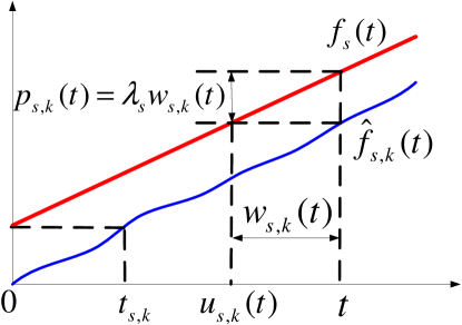
Fig. 1 describes the relations between the variables.

Proof:

Since the first part, i.e., that the two conditions are equivalent, is straightforward from the definition of fluid limits and (4), we focus on the second part, i.e., if $\hat{f}_{s,k}(t_{s,k})>f_{s}(0)$, then (32) follow.

Suppose that $\hat{f}_{s,k}(t_{s,k})>f_{s}(0)$. Then, by the definition of $u_{{s,k}}(t)$, we have $\hat{f}_{s,k}(t)=f_{s}(u_{{s,k}}(t))$, for all $t\geq t_{s,k}$. From (22), (23) and (24), we obtain that

$$\begin{split}p_{s,k}(t)&=f_{s}(t)-\hat{f}_{s,k}(t)\\ &=(f_{s}(0)+\lambda_{s}t)-(f_{s}(0)+\lambda_{s}u_{{s,k}}(t))\\ &=\lambda_{s}\cdot\left(t-u_{{s,k}}(t)\right)\\ &=\lambda_{s}w_{{s,k}}(t).\end{split}$$

∎

Proof:

We prove stability using standard Lyapunov techniques Let $V(\vec{q}(t))$ denote the Lyapunov function defined as

$$\textstyle V(\vec{q}(t))\triangleq\frac{1}{2}\sum_{({s,k})\in\mathcal{P}}\left(q_{s,k}(t)\right)^{2}.$$ (33)

From the results of Lemmas 1 and 3, to show positive recurrence, we only need to prove that for any $\zeta>0$, there exists a finite time $T_{1}>0$ such that for any fluid limit with $\|\vec{q}(0)\|\leq 1$, we have

$$\|\vec{q}(t)\|\leq\zeta,$$ (34)

for all time $t\geq T_{1}$. To show the above, it is sufficient to show that for any $\zeta_{1}>0$, there exists $\zeta_{2}>0$ such that $V(\vec{q}(t))\geq\zeta_{1}$ implies $\frac{D^{+}}{dt^{+}}V(\vec{q}(t))\leq-\zeta_{2}$ for any regular time $t\geq 0$, where $\frac{D^{+}}{dt^{+}}V(\vec{q}(t))=\lim_{\delta\downarrow 0}\frac{V(\vec{q}(t+\delta))-V(\vec{q}(t))}{\delta}$.

Suppose $\vec{\lambda}$ is strictly inside $\Lambda^{*}$, then there exists a vector $\vec{\phi}\in Co(\mathcal{M}_{\mathcal{P}})$ such that $\vec{\lambda}<\vec{\phi}$, i.e., $\lambda_{s}<\phi_{{s,k}}$ for all $({s,k})\in\mathcal{P}$. Since $\vec{q}(t)$ is differentiable, then for any regular time $t\geq 0$, we can obtain the derivative of $V(\vec{q}(t))$ as

$$\begin{split}\textstyle\frac{D^{+}}{dt^{+}}&V(\vec{q}(t))\\ \stackrel{{\scriptstyle(a)}}{{=}}&\textstyle\sum_{({s,k})\in\mathcal{P}}q_{s,k}(t)\cdot\left(\psi_{s,k-1}(t)-\pi_{s,k}(t)\right)\\ \stackrel{{\scriptstyle(b)}}{{\leq}}&\textstyle\sum_{({s,k})\in\mathcal{P}}q_{s,k}(t)\cdot\left(\pi_{s,k-1}(t)-\pi_{s,k}(t)\right)\\ =&\textstyle\sum_{({s,k})\in\mathcal{P}}\Delta q_{s,k}(t)\cdot\lambda_{s}\\ ~{}&\textstyle-\sum_{({s,k})\in\mathcal{P}}\Delta q_{s,k}(t)\cdot\pi_{s,k}(t)\\ =&\textstyle\sum_{({s,k})\in\mathcal{P}}\Delta q_{s,k}(t)\cdot\left(\lambda_{s}-\phi_{s,k}\right)\\ ~{}&+\textstyle\sum_{({s,k})\in\mathcal{P}}\Delta q_{s,k}(t)\cdot(\phi_{s,k}-\pi_{s,k}(t)),\\ \end{split}$$ (35)

where (a) and (b) are from (29) and (25), respectively.

Note that $q_{s,k}(t)\leq{H}^{\max}\max_{({r,j})\in\mathcal{P}}\Delta q_{r,j}(t)$, for any $({s,k})\in\mathcal{P}$. Hence, we have $V(\vec{q}(t))\leq\frac{1}{2}|S|{H}^{\max}({H}^{\max}\max_{({r,j})\in\mathcal{P}}\Delta q_{r,j}(t))^{2}$. Let us choose $\zeta_{3}=\sqrt{\frac{2\zeta_{1}}{|S|({H}^{\max})^{3}}}$, then $V(\vec{q}(t))\geq\zeta_{1}$ implies $\max_{({r,j})\in\mathcal{P}}\Delta q_{r,j}(t)\geq\zeta_{3}$. Since $\vec{\lambda}<\vec{\phi}(t)$ and $\Delta q_{s,k}(t)\geq 0$ for all $({s,k})\in\mathcal{P}$, then in the final result of (35), we can conclude that the first term is bounded as follows:

$$\begin{split}\textstyle\sum_{({s,k})\in\mathcal{P}}\Delta q_{s,k}(t)\cdot\left(\lambda_{s}-\phi_{s,k}\right)&\textstyle\leq-\zeta_{3}\min_{s,k}(\phi_{s,k}-\lambda_{s})\\ &\triangleq-\zeta_{2}<0,\end{split}$$

and that the second term becomes non-positive due to the following. Since Q-BP chooses schedules that maximize the queue differential weight sum (7), then we have that

$$\textstyle\vec{\pi}(t)\in\operatornamewithlimits{argmax}_{\vec{\phi}\in Co(\mathcal{M}_{\mathcal{P}})}\sum_{({s,k})\in\mathcal{P}}\Delta q_{s,k}(t)\cdot\phi_{s,k},$$

which implies that

$$\textstyle\sum_{({s,k})\in\mathcal{P}}\Delta q_{s,k}(t)\cdot\phi_{s,k}\leq\sum_{({s,k})\in\mathcal{P}}\Delta q_{s,k}(t)\cdot\pi_{s,k}(t),$$

for all $\vec{\phi}\in Co(\mathcal{M}_{\mathcal{P}})$. Therefore, this shows that $V(\vec{q}(t))\geq\zeta_{1}$ implies $\frac{D^{+}}{dt^{+}}V(\vec{q}(t))\leq-\zeta_{2}$. Then, it immediately follows that for any $\zeta>0$, there exists a finite time $T_{1}>0$ such that for any fluid limit with $\|\vec{q}(0)\|\leq 1$, we have $\|\vec{q}(t)\|\leq\zeta$ for any time $t\geq T_{1}$. Also, we have

$$p_{s,k}(t)\leq\|\vec{q}(t)\|\leq\zeta,$$ (36)

for all $(s,k)\in\mathcal{P}$. Let us choose $T_{1}$ large enough, then it follows from (20), (22) and (36) that

$$\hat{f}_{s,k}(T_{1})=f_{s}(T_{1})-p_{s,k}(T_{1})>f_{s}(0),$$

for all $(s,k)\in\mathcal{P}$ and for any time $t\geq T_{1}$. Hence, we have (32) from Lemma 3, and thus, we have

$$\begin{split}\|\vec{q}(t)\|+\|\vec{w}\|&\stackrel{{\scriptstyle(a)}}{{\leq}}\|\vec{q}(t)\|+\frac{1}{\min_{s}\lambda_{s}}\|\vec{p}(t)\|\\ &\stackrel{{\scriptstyle(b)}}{{\leq}}\left(1+\frac{|S|{H}^{\max}}{\min_{s}\lambda_{s}}\right)\zeta\\ &\triangleq\epsilon_{1},\end{split}$$

where (a) and (b) are from (32) and (36), respectively. We can make $\epsilon_{1}$ arbitrarily small by choosing small enough $\zeta$.

Now, consider any fixed sequence of processes $\{\frac{1}{x}\mathcal{X}^{(x)}(xt),x=1,2,\cdots\}$ (for simplicity also denoted by $\{x\}$). Hence, for any fixed $\epsilon_{1}>0$, we can always choose a large enough integer $T>0$ such that for any subsequence $\{{x_{n}}\}$ of $\{x\}$, there exists a further (sub)subsequence $\{{x_{n_{j}}}\}$ such that

$$\textstyle\lim_{j\rightarrow\infty}\frac{1}{{x_{n_{j}}}}\|\mathcal{X}^{({x_{n_{j}}})}({x_{n_{j}}}T)\|=\|\vec{q}(T)\|+\|\vec{w}(T)\|\leq\epsilon_{1}$$

almost surely. This in turn implies (for small enough $\epsilon_{1}$) that

$$\textstyle\limsup_{x\rightarrow\infty}\frac{1}{x}\|\mathcal{X}^{(x)}(xT)\|\leq\epsilon_{1}\triangleq 1-\epsilon<1$$ (37)

almost surely. This is because there must exist a subsequence of $\{x\}$ that converges to the same limit as $\limsup_{x\rightarrow\infty}\frac{1}{x}\|\mathcal{X}^{(x)}(xT)\|$.

One can readily show that the sequence $\{\frac{1}{x}\|\mathcal{X}^{(x)}(xT)\|,x=1,2,\cdots\}$ is uniformly integrable using standard techniques by invoking the Dominated Convergence Theorem and so the details are omitted here. Then, the almost sure convergence in (37) along with uniform integrability implies the following convergence in the mean:

$$\textstyle\limsup_{x\rightarrow\infty}\mathbf{E}[\frac{1}{x}\|\mathcal{X}^{(x)}(xT)\|]\leq 1-\epsilon.$$

Since the above convergence holds for any sequence of processes $\{\frac{1}{x}\|\mathcal{X}^{(x)}(x\cdot),x=1,2,\cdots\}$, the condition of (10) in Lemma 1 is satisfied. This completes the proof. ∎

IV Delay-based Back-Pressure Algorithm

IV-A Algorithm Description

In this section, we develop the Delay-based Back-Pressure (D-BP) policy, and in Section IV-B, we prove that it is throughput optimal. A similar delay-based approach has appeared first in [12] for single-hop networks. However, as mentioned earlier, when packets travel multiple hops before leaving the system, the analytical approach in [12] (i.e., using HOL delay in the queue as the metric) cannot capture queueing dynamics of multihop traffic and the resultant solutions cannot guarantee the linear relation. We will carefully design link weights using a new delay metric, and re-establish the linear relation between queue lengths and delays in the fluid limits for multihop traffic.

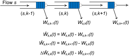
Recall that $W_{{s,k}}(t)$ denotes the sojourn time of the HOL packet of queue $Q_{{s,k}}(t)$ in the network, where the time is measured from the time when the packet arrives in the network. We define the delay metric $\hat{W}_{s,k}(t)$ as

$$\hat{W}_{s,k}(t)\triangleq W_{{s,k}}(t)-W_{s,k-1}(t),$$ (38)

and also define delay differential as

$$\Delta\hat{W}_{s,k}(t)\triangleq\hat{W}_{s,k}(t)-\hat{W}_{s,k+1}(t).$$ (39)

The relations between these delay metrics are illustrated in Fig. 2. We specify the back-pressure algorithm with the new delay metric as follows.

Delay-based Back-Pressure (D-BP) algorithm:

$$\textstyle\vec{M}^{*}\in\operatornamewithlimits{argmax}_{\vec{M}\in\mathcal{M}_{\mathcal{P}}}\sum_{({s,k})\in\mathcal{P}}\Delta\hat{W}_{s,k}(t)\cdot M_{s,k}.$$ (40)

D-BP computes the weight of $({s,k})$ as the delay differential $\Delta\hat{W}_{s,k}(t)$ and solves the MaxWeight problem, i.e., finds a set of non-interfering link-flow-pairs that maximizes weight sum. Ties can be broken arbitrarily if there is more than one schedule that has the largest weight sum. An intuitive interpretation of the new delay metric $\hat{W}_{s,k}(t)$ is as follows. Note that the queue length $Q_{s,k}(t)$ is roughly the number of packets arriving at the source node of flow $s$ during the time slots between $[U_{s,k}(t),U_{s,k}(t)+\hat{W}_{s,k}(t))$, and from the SLLN, $Q_{s,k}(t)$ is on the order of $\lambda_{s}\hat{W}_{s,k}(t)$ when $\hat{W}_{s,k}(t)$ is large. Hence, a large $\hat{W}_{s,k}(t)$ implies a large queue length $Q_{s,k}(t)$, and similarly, a large delay differential $\Delta\hat{W}_{s,k}(t)$ implies a large queue length differential $\Delta Q_{s,k}(t)$. Therefore, being favorable to the delay weight sum in (40) is in some sense “equivalent” to being favorable to the queue length weight sum in (7) as Q-BP. We later formally establish the linear relation between the fluid limits of queue lengths and delays in Section IV-B.

We highlight here that the last packet problem can be solved by the D-BP scheme using our proposed delay metric. Let us focus on the source nodes first. Suppose that at the source node of flow $s$, there are a finite number of packets waiting to be transmitted and there are no further packet arrivals. From the definition of (38) and the fact that $W_{s,0}(t)=0$, we have $\hat{W}_{s,1}(t)=W_{s,1}(t)$. If some of the packets are stuck at the source node, the delay metric $\hat{W}_{s,1}(t)$ keeps increasing with time. On the other hand, $\hat{W}_{s,2}(t)=W_{s,2}(t)-W_{s,1}(t)$ is equal to the inter-arrival time between two packets and does not increase with time, in particular because some packets at the source node are not served. Hence, the delay differential $\Delta\hat{W}_{s,1}(t)=\hat{W}_{s,1}(t)-\hat{W}_{s,2}(t)$ also increases with time. This implies that under DBP, the increasing delay will eventually “push” all the packets that are waiting at the source node to the second-hop link. After all the packets leave the source node, we can observe similar procedure at the transmitting node of the second-hop link: since $Q_{s,1}(t)=0$ and $W_{s,1}(t)=0$, we have $\hat{W}_{s,2}(t)=W_{s,2}(t)$. Repeating the same argument, we can conclude that all the packets will ultimately be “pushed” to the destination node of flow $s$.

Figure 2: Delay differentials using new delay metric.

Recall that $U_{{s,k}}(t)$ denotes the time when the HOL packet of $Q_{s,k}$ arrives in the network (or the source node, rather than the current node). We let $U^{\prime}_{{s,k}}(t)$ denote the time when the packet that arrives (in the network or the source node) immediately after the HOL packet of $Q_{s,k}$ arrives in the network. Let $B_{{s,k}}(t)\triangleq U^{\prime}_{{s,k}}(t)-U_{{s,k}}(t)$ denote the inter-arrival time between the HOL packet of $Q_{s,k}$ and the packet that arrives immediately after it. Clearly, D-BP will not schedule link-flow-pair $({s,k})$ if

$$\hat{W}_{s,k}(t)-\hat{W}_{s,k+1}(t)<0.$$

Hence, if link-flow-pair $({s,k})$ is scheduled, it must satisfy $\hat{W}_{s,k}(t)-\hat{W}_{s,k+1}(t)\geq 0$. Moreover, the delay $\hat{W}_{s,k}(t)$ can decrease by at most $B_{{s,k}}(t)$ within one time slot, and the delay $\hat{W}_{s,k+1}(t)$ can increase by at most $B_{{s,k}}(t)$ within one time slot, due to the assumption of unit link capacity (a similar argument also holds with non-unit link rates). Therefore, if inequality

$$\hat{W}_{s,k}(t)\geq\hat{W}_{s,k+1}(t)-2B_{{s,k}}(t)$$ (41)

initially holds for all $({s,k})$ at time slot 0, then the inequality holds for all time slot $t\geq 0$. This further leads to

$$\hat{w}_{s,k}(t)\geq\hat{w}_{s,k+1}(t),~{}\text{i.e.,}~{}\Delta\hat{w}_{s,k}(t)\geq 0,$$ (42)

for all (scaled) time $t\geq 0$, in the fluid limits, from the convergence of (18) and that $\frac{1}{{x_{n_{j}}}}B^{({x_{n_{j}}})}_{{s,k}}({x_{n_{j}}}t)\rightarrow$ $0$, as ${x_{n_{j}}}\rightarrow\infty$ (otherwise we will arrive a contradiction with the assumption on the arrival process, i.e., it satisfies the Strong Law of Large Numbers). Recall that we assume that all queues on each route are empty at time slot 0, except for the first queue, then (41) and (42) follow.

IV-B Throughput-Optimality

The following lemma provides the linear relation between queue lengths and delays in the fluid limits.

Lemma 4

For any fixed $t_{s,k}>0$, if $\hat{f}_{s,k}(t_{s,k})$ $>$ $f_{s}(0)$ for every link-flow-pair $({s,k})\in\mathcal{P}$, then we have

$$q_{s,k}(t)=\lambda_{s}\hat{w}_{s,k}(t),$$ (43)

for all $t\geq t_{s,k}$, with probability one.

Proof:

It follows immediately from Lemma 3. ∎

We emphasize the importance of (43). Lemma 4 implies that after a finite time (i.e., $\max_{({s,k})\in\mathcal{P}}t_{s,k}$), the queue lengths are $\lambda_{s}$ times delays in the fluid limit model. Then the schedules of D-BP are very similar to those of Q-BP, which implies that D-BP achieves the optimal throughput region $\Lambda^{*}$. In the following, we show that the condition of Lemma 4 indeed holds, i.e., such a finite time exists.

Lemma 5

Consider a system under the D-BP policy. Then for $\vec{\lambda}$ strictly inside $\Lambda^{*}$, there exists a finite time $T>0$ such that the fluid limits satisfy the following property with probability one,

$$\hat{f}_{s,k}(T)>f_{s}(0),$$ (44)

for all link-flow-pairs $({s,k})\in\mathcal{P}$.

We can prove Lemma 5 by induction following the techniques described in Lemma 7 of [12]. The formal proof is provided in Appendix B. We next outline an informal discussion, which highlights the main idea of the proof. First, we consider the base case. D-BP chooses one of the feasible schedules in $\mathcal{M}_{\mathcal{P}}$ (we omit the term “feasible” in the following, whenever there is no confusion) at each time slot. Each schedule receives a fraction of the total time and there must exist a schedule that receives at least $\frac{1}{|\mathcal{M}_{\mathcal{P}}|}$ fraction of the total time. Thus, after a large enough time $T_{1}>0$, there must exist a schedule $\vec{M}^{*}$ that is chosen for at least $\frac{T_{1}}{|\mathcal{M}_{\mathcal{P}}|}$ amount of time. The number of initial packets of $\vec{M}^{*}$ is bounded from (20), thus, for a large enough $T_{1}$, all initial “fluid” of at least one link-flow-pair of $\vec{M}^{*}$ must be completely served, i.e., $\hat{f}_{s,k}(T_{1})>f_{s}(0)$, for at least one $({s,k})$ with $M^{*}_{{s,k}}=1$.

Next, we consider the inductive step. Suppose there exists a $T_{l}>0$, such that for at least one subset $S_{l}\subset\mathcal{P}$ of cardinality $l$, we have

$$\hat{f}_{s,k}(T_{l})>f_{s}(0),$$ (45)

for all $({s,k})\in S_{l}$. Then there exists $T_{l+1}\geq T_{l}$ such that

$$\hat{f}_{s,k}(T_{l+1})>f_{s}(0),$$ (46)

holds for all link-flow-pairs $({s,k})$ within at least one subset $S_{l+1}\subset\mathcal{P}$ of cardinality $l+1$. Since flows travel hop-by-hop, packets that have been served by one link must have been served by the link at the previous hop (of the flow that the packets belong to). Hence, if $(s,k)\in S_{l}$, we must have $(s,k-1)\in S_{l}$. Repeating the argument, if $(s,k)\in S_{l}$, we have $(s,i)\in S_{l}$ for $1\leq i\leq k$. Let

$$\begin{split}S^{*}_{l}\triangleq\{({r,j})~{}|~{}&({r,j})\notin S_{l},({r,j}-1)\in S_{l},~{}\text{for}~{}j>1;\\ &~{}\text{or}~{}({r,j})\notin S_{l},~{}\text{for}~{}j=1\}\end{split}$$ (47)

denote the set of link-flow-pairs $({r,j})$ such that $({r,j})\in\mathcal{P}\backslash S_{l}$ is the closest hop to the source of $r$. To avoid unnecessary complications, we discuss the induction step for $l=1$. The generalization for $l>1$ is straightforward. We show that for given $S_{1}$ and $T_{1}$, there exists a finite time $T_{2}\geq T_{1}$ such that (46) with $T_{2}$ holds for at least two different link-flow-pairs.

Let $({\hat{s},\hat{k}})$ denote the link-flow-pair that satisfies (45) with $T_{1}$. Since $({\hat{s},\hat{k}})\in S_{l}$ implies $(\hat{s},i)\in S_{l}$ for all $1\leq i\leq\hat{k}$, we must have $\hat{k}=1$ and $S_{1}=\{(\hat{s},1)\}$. From (47), we have that

$$S_{1}^{*}=\{(r,1)~{}|~{}r\in\mathcal{S}\backslash\{\hat{s}\}\}\cup N_{\hat{s}},$$ (48)

where $N_{\hat{s}}=\{(\hat{s},2)\}$ if ${H}(\hat{s})>1$, and $N_{\hat{s}}=\emptyset$ if ${H}(\hat{s})=1$. We discuss only the case that ${H}(\hat{s})>1$, and the other case can be easily shown following the same line of analysis. Now suppose that

$$\hat{f}_{{r,j}}(t)\leq f_{r}(0),~{}\text{for all}~{}({r,j})\in\mathcal{P}\backslash S_{1},~{}\text{and all}~{}t\geq 0,$$ (49)

i.e., for all the link-flow-pairs except those of $S_{1}$, the total amount of service up to time $t$ is no greater than the amount of the initial fluid for all $t\geq 0$. We show that this assumption leads to a contradiction, which completes the induction step.

From the base case and Lemma 4, we have $q_{\hat{s},1}(t)$ $=$ $\lambda_{\hat{s}}\hat{w}_{\hat{s},1}(t)$ for all $t\geq T_{1}$. We view the subset of link-flow-pairs $S_{1}$ as a generalized system, and consider the time slots when there is at least one packet transmission from the outside of $S_{1}$, i.e., $({r,j})\in\mathcal{P}\backslash S_{1}$. For each such time slot, we say that the time slot is unavailable to $S_{1}$.

1. The number of such unavailable time slots is bounded from the above by ${x_{n_{j}}}$, since at every such time slot, at least one initial packet will be transmitted and the total number of initial packets is bounded by $\|\vec{Q}(0)\|\leq{x_{n_{j}}}$ from (9). Hence, the amount of (scaled) time unavailable to $S_{1}$ is bounded by $\|\vec{q}(0)\|\leq 1$.

2. Since the amount of (scaled) time unavailable to $S_{1}$ is bounded, there exists a sufficiently large $t\geq T_{1}$ such that the fraction of time that is given to $({r,j})\in\mathcal{P}\backslash S_{1}$ is negligible, and we must have $\hat{w}_{\hat{r},\hat{j}}(t)=\Theta(1)$ and $\Delta\hat{w}_{\hat{r},\hat{j}}(t)=\Theta(1)$ for $(\hat{r},\hat{j})\in\mathcal{P}\backslash(S_{1}\cup S_{1}^{*})$.

3. Then, we can restrict our focus on the generalized system $S_{1}$ to time $t\geq T_{1}$, and ignore the time that is unavailable to $S_{1}$. Then Q-BP and D-BP are in some sense “equivalent” in the generalized system $S_{1}$ for $t\geq T_{1}$ with the following properties: First, Q-BP will stabilize the system if the arrival rate vector is strictly inside $\Lambda^{*}$. Second, since the linear relation (43) holds for all link-flow-pairs in $S_{1}$ from Lemma 4, D-BP will schedule links similar to Q-BP and also stabilizes the generalized system $S_{1}$.

4. Now let us focus on $S_{1}^{*}$. Link-flow-pairs in $S_{1}^{*}$ must have some initial fluid at $t\geq T_{1}$ because $S_{1}\cap S_{1}^{*}=\emptyset$. On the other hand, the generalized network $S_{1}$ is stable. This implies that the delay metrics of link-flow-pairs in $S_{1}^{*}$ should increase on the same order as we increase $t$, i.e., $\hat{w}_{r^{*},j^{*}}(t)=\Theta(t)$ for $(r^{*},j^{*})\in S_{1}^{*}$. Then we have $\Delta\hat{w}_{r^{*},j^{*}}(t)=\Theta(t)$, since $\hat{w}_{r^{*},j^{*}+1}(t)=\Theta(1)$ from $(r^{*},j^{*}+1)\in\mathcal{P}\backslash(S_{1}\cup S_{1}^{*})$ and 2). Since the delay differentials $\Delta\hat{w}_{{s,k}}(t)$ for all $({s,k})\in S_{1}$ and $\Delta\hat{w}_{\hat{r},\hat{j}}(t)$ for all $(\hat{r},\hat{j})\in\mathcal{P}\backslash(S_{1}\cup S_{1}^{*})$ are bounded above from stability of $S_{1}$ and 2), respectively, D-BP will choose link-flow-pairs in the set of $S_{1}^{*}$ for most of time for a sufficiently large $t$. This implies that the amount of time unavailable to $S_{1}$ is $\Theta(t)$, which contradicts with our previous statement in 1) that the fraction of time that is given to $({r,j})\in\mathcal{P}\backslash S_{1}$ is negligible.

We provide the detailed proof of Lemma 5 in Appendix B.

We then present throughput-optimality of D-BP in the following proposition.

Proposition 6

D-BP can support any traffic with arrival rate vector that is strictly inside $\Lambda^{*}$.

Proof:

We show the stability using fluid limits and standard Lyapunov techniques. From Lemmas 4 and 5, we obtain the key property for proving throughput-optimality of D-BP in Eq. (43), i.e., after a finite time, there is a linear relation between queue lengths and delays in the fluid limit model. We start with the following quadratic-form Lyapunov function,

$$\textstyle V(\vec{q}(t))\triangleq\frac{1}{2}\sum_{({s,k})\in\mathcal{P}}\frac{\left(q_{s,k}(t)\right)^{2}}{\lambda_{s}}.$$ (50)

Following the line of analysis in the proof for Proposition 2, we can show that for any $\zeta_{1}>0$, there exist $\zeta_{2}>0$ and a finite time $T>0$ such that $V(\vec{q}(t))\geq\zeta_{1}$ implies $\frac{D^{+}}{dt^{+}}V(\vec{q}(t))\leq-\zeta_{2}$ for any regular time $t\geq T$, if the underlying scheduler maximizes $\sum_{s,k}\frac{\Delta q_{s,k}(t)}{\lambda_{s}}\cdot\pi_{s,k}(t)$. Then, by applying the linear relation (43), we can see that D-BP indeed satisfies such a condition, and obtain the results. We omit the detailed proof since it mirrors the derivations in Proposition 2. ∎

V Greedy Algorithms

It is well known that the schemes (e.g., Q-BP and D-BP) based on the back-pressure techniques are complex to implement because they involve computing a MaxWeight component, which in general is NP-hard [19]. Hence, although D-BP operates efficiently and achieves the optimal throughput region, it could be difficult to implement in practice. Therefore, we are interested in simpler approximations of D-BP that can achieve a guaranteed fraction of the optimal performance. The Delay-based Greedy Maximal Scheduling (D-GMS) algorithm is a good candidate approximation algorithm. A Greedy Maximal Scheduling (GMS) algorithm [32, 23, 33, 26] (which is also known as Longest Queue First (LQF)) operates (in the scenarios with single-hop traffic) as follows: at each time slot $t$, starts with an empty schedule; first picks a link $l$ with the maximum weight (e.g., queue length or delay); adds $l$ into the schedule, and disables other links that interfere with $l$; next picks a link $l^{\prime}$ with the maximum weight from the remaining set of links, adds $l^{\prime}$ into the schedule, and disables other links that interfere with $l^{\prime}$; and continues this process until all links are either chosen or disabled. All chosen links will be scheduled during time slot $t$. Note that any schedule obtained by GMS is maximal.

GMS has been extensively studied due to its low complexity [23], distributed implementations [34] (or distributed approximations [35]) and empirically observed good performance [22]. It was first shown in [32] that GMS is throughput-optimal in networks where the so-called local pooling condition is satisfied. The authors of [21, 33] generalize the idea of local pooling to $\sigma$-local pooling, where $\sigma$ is a topological notion depending on the underlying network topology and is called the local pooling factor. There, the authors show that GMS can achieve a $\sigma$-fraction of the optimal throughput region. On the other hand, in [36, 37], the local pooling condition is generalized to the scenarios with multihop traffic, i.e., GMS is throughput-optimal in networks where the multihop local-pooling condition is satisfied. Next, we will discuss the performance limits of D-GMS.

Algorithm 1 Greedy Maximal Scheduling (GMS) Algorithm

1:procedure GMS($\mathcal{P},x$)

2:     $M\leftarrow\emptyset$

3:     $\mathcal{P}^{\prime}\leftarrow\mathcal{P}$

4:     while $\mathcal{P}^{\prime}\neq\emptyset$ do

5:         pick a link-flow-pair $({s,k})$ with maximum weight: $x({s,k})=\max_{({r,j})\in\mathcal{P}^{\prime}}x({r,j})$

6:         $M\leftarrow M\cup\{({s,k})\}$

7:         $\mathcal{P}^{\prime}\leftarrow\mathcal{P}^{\prime}\backslash I({s,k})$

8:     end while

9:end procedure

To generalize the GMS algorithm to settings with multihop traffic, we consider link-flow-pairs. We let $x({s,k})$ denote the weight of link-flow-pair $({s,k})\in\mathcal{P}$, and conclude the procedure of GMS in Algorithm 1. We then describe the operations of D-GMS and its queue-length-based counterpart (called Q-GMS) in the following.

Delay-based Greedy Maximal Scheduling (D-GMS) Algorithm: At each time slot $t$, the algorithm sets the weight of each link-flow-pair to the delay differential, i.e.,

$$x({s,k})\leftarrow\Delta\hat{W}_{s,k}(t),~{}\text{for all}~{}({s,k})\in\mathcal{P},$$ (51)

and finds its schedule in decreasing order of weight conforming to the underlying interference constraints, by applying Algorithm 1.

Queue-length-based Greedy Maximal Scheduling (Q-GMS) Algorithm: At each time slot $t$, the algorithm sets the weight of each link-flow-pair to the queue-length differential, i.e.,

$$x({s,k})\leftarrow\Delta Q_{s,k}(t),~{}\text{for all}~{}({s,k})\in\mathcal{P},$$ (52)

and finds its schedule by applying Algorithm 1.

We characterize the throughput performance of D-GMS in the following proposition.

Proposition 7

The achievable throughput region of D-GMS is no smaller than that of Q-GMS.

We omit the proof here, since it follows the similar line of analysis for D-BP to establish the linear relation between queue lengths and delays in the fluid limits, and the result can then be obtained by applying the techniques used in [36, 37].

VI Numerical Results

In this section, we first highlight the last packet problem for the queue-length-based back-pressure algorithm. The last packet problem implies that flows that lack packet arrivals at subsequent time may experience excessive delays under Q-BP, which is later confirmed in the simulations. Then, we compare throughput and delay performance of Q-BP and D-BP in a grid network topology under the 2-hop interference model. Finally, we compare throughput performance of Q-GMS and D-GMS in a size-6 ring network under the 1-hop interference model.

(a) “H”-type network topology

(b) HOL delay of short flow $(2\rightarrow 4\rightarrow 6)$ when $\lambda=3$

Figure 3: Illustration of the last packet problem under Q-BP.

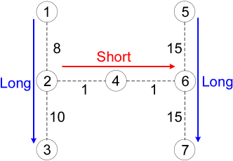
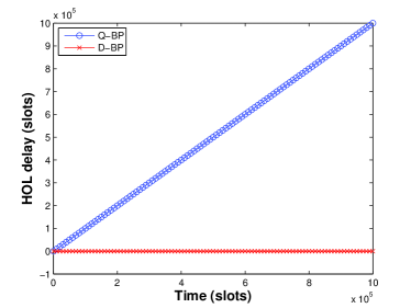
We first show the last packet problem of Q-BP through simulations. We observe that several last packets of a short flow (that carry a finite amount of data) may get stuck, which could cause excessive delays. We consider a scenario consisting of 7 nodes and 6 links as shown in Fig. 3(a), where nodes are represented by circles and links are represented by dashed lines with their associated link capacities. We assume a time-slotted system. We establish three flows: one short flow ($2\rightarrow 4\rightarrow 6$) and two long flows ($1\rightarrow 2\rightarrow 3$) and ($5\rightarrow 6\rightarrow 7$). The short flow arrives in the network with 10 packets at time 0. The long flows have an infinite amount of data and keep injecting packets at the source nodes following Poisson distribution with mean rate $\lambda$ at each time slot. Numerical calculation shows that the feasible rate under the 2-hop interference should satisfy that $\lambda\leq 4.44$. We conduct our simulation for $10^{6}$ time slots, and plot time traces of HOL delay of the short flow when $\lambda=3$. Fig. 3(b) illustrates the results that the delay increases linearly with time under Q-BP, which implies that several last packets of the short flow are excessively delayed. On the other hand, D-BP succeeds in serving the short flow and keeps the delay close to 0. This also implies that certain flows whose queue lengths do not increase due to lack of future arrivals (or whose inter-arrival times between groups of packets are very large) may experience a large delay under Q-BP, which will be confirmed in the following simulations.

(a) Grid network topology

(b) Average queue length

Figure 4: Performance of scheduling algorithms for multihop traffic following Poisson distribution.

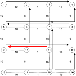
Next, we evaluate the throughput performance of different schedulers in a grid network that consists of 16 nodes and 24 links as shown in Fig. 4(a), where nodes and links are represented by circles and dashed lines, respectively, with link capacity. We establish 9 multihop flows that are represented by arrows. Let $\lambda_{1}=0.1$ and $\lambda_{2}=1$. At each time slot, there is a file arrival with probability $p=0.01$ for flow ($11\rightarrow 10\rightarrow 9$) (represented by the red thick arrow in Fig. 4(a)), and the file size follows Poisson distribution with mean rate $\rho\lambda_{1}/p$. Note that flow ($11\rightarrow 10\rightarrow 9$) has bursty arrivals with a small mean rate (we simply call it the bursty flow in the following part). All the other 8 flows have packet arrivals following Poisson distribution with mean rate $\rho\lambda_{2}$ at each time slot. Although these flows share the same stochastic property with an identical mean arrival rate $\rho\lambda_{2}$, uniform patterns of traffic are avoided by carefully setting the link capacities and placing the flows with different number of hops in an asymmetric manner.

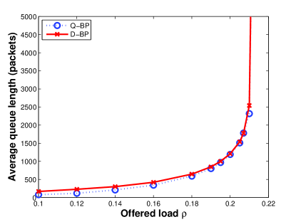
We evaluate the scheduling performance by measuring average total queue lengths in the network over time. Fig. 4(b) illustrates average queue lengths under different offered loads to examine the performance limits of scheduling schemes. Each result represents an average of 10 simulation runs with independent stochastic arrivals, where each run lasts for $10^{6}$ time slots. Since the optimal throughput region is defined as the set of arrival rates under which the queue lengths remain finite, we can consider the traffic load, under which the queue length increases rapidly, as the boundary of the optimal throughput region. Fig. 4(b) shows that D-BP achieves the same throughput region as Q-BP, thus supporting the theoretical results on throughput performance.

Figure 5: Delay distribution of the bursty flow under $\rho=0.2$.

Figure 6: Mean delay, the 1st and 5th percentile delay of the bursty flow ($11\rightarrow 10\rightarrow 9$) over offered loads.

Although Q-BP and D-BP perform similarly in terms of the average queue length (or average delay due to Little’s Law) over the network, the tail of the delay distribution of Q-BP could be substantially longer because certain flows are starved. This could cause enormous unfairness between flows, resulting in very poor QoS for certain flows.

Note that although a bursty flow is a long flow that has an infinite amount of data, the arrivals occur in a dispersed manner (i.e., the inter-arrival times between groups of packets are very large) and we can view this bursty flow as consisting of many short flows. Thus, we expect that the bursty flow may experience a very large delay under Q-BP. This is because the bursty flow lacks subsequent packet arrivals over long periods of time, which does not allow the queue-lengths to grow, and thus contributes to the long tail of the delay distribution. However, this phenomenon may not manifest itself in terms of a higher average delay for Q-BP, as can be observed in Fig. 4(b), because the amount of data corresponding to the bursty flow in the simulation is small compared to the other flows. On the other hand, D-BP can achieve better fairness by scheduling the links based on delays and not starving bursty or variable flows. We confirm this in the following observations.

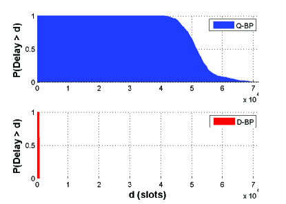
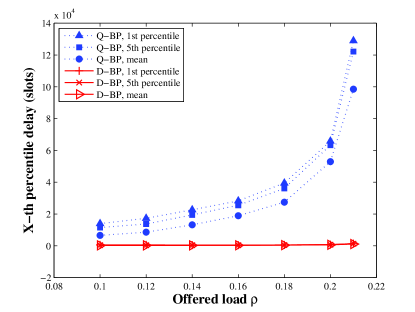
Fig. 5 illustrates the effectiveness of using D-BP over Q-BP in terms of how each scheme affects the delay distribution of bursty flows. We set $\rho=0.2$. The results show that the tail of the delay distribution under D-BP vanishes much faster than Q-BP. Further, we plot the mean delay, the 1st and 5th percentile delay of the bursty flow over offered loads in Fig. 6. All these delays under D-BP are substantially less than under Q-BP, which implies that D-BP successfully eliminates the excessive packet delays. This confirms that, Q-BP causes a substantially long tail for the delay distribution of the network due to the starvation of the bursty flow, while D-BP overcomes this and achieves better fairness among the flows by scheduling the links based on delays.

(a) A size-6 ring network topology

(b) Average queue length

Figure 7: Performance comparison of Q-BP, D-BP, Q-GMS and D-GMS for multihop traffic under the 1-hop interference model.

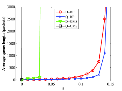
Finally, we consider a size-6 ring network topology under the 1-hop interference model as shown in Fig. 7(a), where links have unit link capacity. We simulate two flows: flow ($1\rightarrow 2\rightarrow 3\rightarrow 4$) and flow ($4\rightarrow 5\rightarrow 6\rightarrow 1$). It is known [21] that Q-GMS is not throughput-optimal in this network, as the local pooling condition is not satisfied (and thus the multihop local pooling is not satisfied from Lemma 7 of [37]). On the other hand, although D-GMS is at least as efficient as Q-GMS, it is not known whether D-GMS can achieve larger throughput in certain scenarios, e.g., in the network in Fig. 7(a).

To see these, we construct a traffic pattern using the idea in [33]. We consider packet arrivals in a frame of 12 time slots. Two flows have the same arrival pattern in each frame. We assume two arrival patterns for each frame. Starting with empty queues at time slot 0, in each frame, the number of exogenous packet arrivals at the source of each flow (i.e., nodes 1 and 4) follows pattern $P_{1}=\{1,0,5,0,\,1,0,5,0,\,1,0,5,0\}$ with probability $\epsilon$, and pattern $P_{2}=\{1,0,0,\,1,0,0,\,1,0,0,\,1,0,0\}$ with probability $(1-\epsilon)$, where $0\leq\epsilon\leq 1$. The average arrival rate vector is then $\vec{\lambda}=(\frac{18}{12}\epsilon+\frac{4}{12}(1-\epsilon))\textbf{e}=(\frac{1}{3}+\frac{7}{6}\epsilon)\textbf{e}$, where e is a dimension-2 vector with all components equal to 1. It is easy to check that $\vec{\lambda}$ lies strictly inside the optimal throughput region when $0\leq\epsilon<\frac{1}{7}$, while Q-GMS cannot stabilize the network under such a traffic pattern for all $\epsilon>0$. Because under Q-GMS, when pattern $P_{2}$ occurs in a frame, all the packets arriving in this frame can be completely served and leave the network by the end of this frame, while pattern $P_{1}$ occurs, none of the packets arriving in this frame leaves the network by the end of this frame. We evaluate the performance of different scheduling policies under the above traffic pattern. For each policy under a fixed $\epsilon$, we take the average over 10 independent experiments, with each run being $10^{7}$ time slots. In Fig. 7(b), we can see that Q-BP and D-BP have finite average queue length for $0\leq\epsilon<\frac{1}{7}=0.143$ and thus achieve the maximum throughput. On the other hand, the average queue length increases linearly with $\epsilon$ under Q-GMS and D-GMS starting from $\epsilon=0$ and $\epsilon=0.04$, respectively. This implies that neither Q-GMS nor D-GMS is throughput-optimal in this setting, while D-GMS achieves larger throughput ($\epsilon<0.04$). To fully characterize the performance limits of D-GMS is an interesting yet challenging problem.

VII Conclusion

In this paper, we developed a throughput-optimal delay-based back-pressure scheduling scheme for multihop wireless networks with fixed routes. We introduced a new delay metric suitable for multihop traffic and established a linear relation between queue lengths and delays in the fluid limits, which plays a key role in the performance analysis and proof of throughput-optimality. Delay-based schemes provide a simple way around the well-known last packet problem that plagues queue-based schedulers, and thus avoid flow starvation. As a result, the excessively long delays that could be experienced by certain flows under queue-based scheduling schemes are eliminated without any loss of throughput. Nonetheless, in this paper, we have only considered the scheduling problem with fixed routes, albeit with multihop flows. The question of whether delay-based schemes under dynamic routing can achieve throughput-optimality is still very much open.

Appendix A Summary of notations

Symbol	Definition
$\mathcal{V}$	set of nodes
$\mathcal{E}$	set of links
$\mathcal{S}$	set of flows
$\mathcal{P}$	set of link-flow-pairs
$\mathcal{M}_{\mathcal{P}}$	set of feasible schedules
$Co(\mathcal{M}_{\mathcal{P}})$	convex hull of $\mathcal{M}_{\mathcal{P}}$
$\Lambda^{*}$	optimal throughput region
${H}(s)$	# of hops on the route of flow $s$
${H}^{\max}$	$\max_{s\in\mathcal{S}}{H}(s)$
$A_{s}(t)$	# of packet arrivals for flow $s$ at time slot $t$
$\lambda_{s}$	mean arrival rate for flow $s$
$F_{s}(t)$	cumulative # of packet arrivals for flow $s$ up to time slot $t$
$Q_{s,k}(t)$	queue length of $Q_{s,k}$ at time slot $t$
$\Pi_{s,k}(t)$	service at $Q_{s,k}$ at time $t$
$\Psi_{s,k}(t)$	# of packet departures at $Q_{s,k}$ at time slot $t$
$P_{s,k}(t)$	$\sum_{i=1}^{k}Q_{s,i}(t)$
$\hat{F}_{s,k}(t)$	cumulative # of packets served at $Q_{s,k}$ up to time slot $t$
$Z_{{s,k},i}(t)$	sojourn time (in the network) of the $i$-th packet of $Q_{s,k}$ at time slot $t$
$W_{s,k}(t)$	sojourn time (in the network) of the HOL packet of $Q_{s,k}$ at time slot $t$, i.e., $Z_{{s,k},1}(t)$
$U_{s,k}(t)$	time when the HOL packet of $Q_{s,k}$ arrives in the network, i.e., $t-W_{s,k}(t)$
$\hat{W}_{s,k}(t)$	$W_{s,k}(t)-W_{s,k-1}(t)$
$\Delta\hat{W}_{s,k}(t)$	$\hat{W}_{s,k}(t)-\hat{W}_{s,k+1}(t)$
$\Delta Q_{s,k}(t)$	$Q_{s,k}(t)-Q_{s,k+1}(t)$
$B_{s,k}(t)$	inter-arrival time (at the system or the source node) between the HOL packet of $Q_{s,k}$ and the packet that arrives immediately after it

TABLE I: Summary of notations

Appendix B Proof of Lemma 5

Proof:

We show that there exists a finite time $T>0$ such that the fluid limits satisfy $\hat{f}_{{s,k}}(T)>f_{s}(0)$ for all link-flow-pairs $({s,k})\in\mathcal{P}$. We prove this by induction. We show that there exists a finite time $T$ with at least one link-flow-pair that satisfies the condition, and for a given set of link-flow-pairs satisfying the condition, at least one additional link-flow-pair will satisfy the condition by increasing $T$.

We first fix an arbitrary $\epsilon_{1}>0$ and define a constant $K_{1}\triangleq\max_{s}{H}(s)+\left(\sum_{s}\lambda_{s}{H}(s)\right)\epsilon_{1}$. In the fluid limit model, we will have

$$f_{s}(\epsilon_{1})=f_{s}(0)+\lambda_{s}\epsilon_{1}>f_{s}(0),~{}\text{for all}~{}s\in\mathcal{S}.$$

Since queue lengths are no greater than the injected amount of data, we have that $p_{{s,k}}(\epsilon_{1})\leq f_{s}(\epsilon_{1})$ for all $({s,k})\in\mathcal{P}$, and thus,

$$\begin{split}\textstyle\sum_{({s,k})\in\mathcal{P}}p_{s,k}(\epsilon_{1})&\leq\textstyle\sum_{({s,k})\in\mathcal{P}}f_{s}(\epsilon_{1})\\ &\leq\textstyle\sum_{s}{H}(s)\left(f_{s}(0)+\lambda_{s}\epsilon_{1}\right)\\ &\leq K_{1},\end{split}$$ (53)

where the last inequality is from Eq. (20): $\sum_{s}f_{s}(0)\leq 1$ and the definition of $K_{1}$. Now we show by induction that there exists a finite time $T$ such that

$$\hat{f}_{s,k}(T)>f_{s}(0),~{}\text{for all link-flow-pairs}~{}({s,k}).$$

Base Case: There exists $T_{1}>0$ such that for at least one link-flow-pair $({s,k})$,

$$\hat{f}_{s,k}(T_{1})\geq f_{s}(\epsilon_{1}).$$ (54)

Let $T_{1}\triangleq\epsilon_{1}+K_{1}$. Suppose that (54) does not hold, i.e., there exists at least one packet that arrives before time slot $\lfloor{x_{n_{j}}}\epsilon_{1}\rfloor+1$ and is not served by the end of time slot $\lfloor{x_{n_{j}}}T_{1}\rfloor$. Hence, at each time slot between $[\lfloor{x_{n_{j}}}\epsilon_{1}\rfloor+1,\lfloor{x_{n_{j}}}T_{1}\rfloor]$, there exists at least one schedule that has positive summed weight. Therefore, the schedule determined by D-BP must serve at least one packet in the original system, otherwise the summed weight of the schedule (that does not serve any packet) is zero, which is not the maximum over all the feasible schedules. Hence, we must have

$$\begin{split}\textstyle\sum_{({s,k})\in\mathcal{P}}\left(\hat{F}^{({x_{n_{j}}})}_{s,k}({x_{n_{j}}}T_{1})-\hat{F}^{({x_{n_{j}}})}_{s,k}({x_{n_{j}}}\epsilon_{1})\right)\\ \textstyle\geq\lfloor{x_{n_{j}}}T_{1}\rfloor-\lfloor{x_{n_{j}}}\epsilon_{1}\rfloor,\end{split}$$

Dividing both sides of the above inequality by ${x_{n_{j}}}$ and letting ${x_{n_{j}}}\rightarrow\infty$, we obtain

$$\textstyle\sum_{({s,k})\in\mathcal{P}}\left(\hat{f}_{s,k}(T_{1})-\hat{f}_{s,k}(\epsilon_{1})\right)\geq K_{1}.$$

Then, from (53), we have

$$\begin{split}\textstyle\sum_{({s,k})\in\mathcal{P}}\hat{f}_{s,k}(T_{1})&\geq\textstyle\sum_{({s,k})\in\mathcal{P}}\hat{f}_{s,k}(\epsilon_{1})+\sum_{({s,k})\in\mathcal{P}}p_{s,k}(\epsilon_{1})\\ &=\textstyle\sum_{({s,k})\in\mathcal{P}}f_{s}(\epsilon_{1}).\end{split}$$

Therefore, $\hat{f}_{s,k}(T_{1})\geq f_{s}(\epsilon_{1})$ for at least one link-flow-pair $({s,k})$.

Inductive Step: Suppose that there exist $T_{l}$ and a subset $S_{l}\subseteq\mathcal{P}$ such that for all $({s,k})\in S_{l}$, we have

$$\hat{f}_{s,k}(T_{l})\geq f_{s}(\epsilon_{1}).$$ (55)

Then there exists $T_{l+1}\geq T_{l}$, where $1\leq l<\sum_{s}{H}(s)$, and a link-flow-pair $(\tilde{s},\tilde{k})\in\mathcal{P}\backslash S_{l}$ such that

$$\hat{f}_{\tilde{s},\tilde{k}}(T_{l+1})\geq f_{\tilde{s}}(\epsilon_{1}).$$ (56)

Further we define $S_{l+1}=S_{l}\cup\{(\tilde{s},\tilde{k})\}$.

We prove the inductive step for $l=1$. The generalization for $l>1$ is straightforward. Hence, we show that for given $S_{1}$ and $T_{1}$, there exists a finite $T_{2}>T_{1}$ such that (56) with $T_{2}$ holds for at least two different link-flow-pairs.

Let $({\hat{s},\hat{k}})$ denote the link-flow-pair that satisfies (55) with $T_{1}$. Then, we have $S_{1}=\{(\hat{s},1)\}$ and can specify the set $S_{1}^{*}$ of link-flow-pairs $(s,k)\in\mathcal{P}\backslash S_{1}$ that is closest to the source of each flow from (48). We illustrate the case that ${H}(\hat{s})>1$, and the other case that ${H}(\hat{s})=1$ can be easily shown following the same line of analysis. Now, we have

$$\hat{f}_{\hat{s},1}(t)\geq f_{\hat{s}}(\epsilon_{1}),~{}\text{for all}~{}t\geq T_{1}.$$

For all the other link-flow-pairs, we observe that

$$\textstyle\sum_{({r,j})\in\mathcal{P}\backslash S_{1}}\left(f_{r}(\epsilon_{1})-\hat{f}_{{r,j}}(T_{1})\right)\leq K_{1}.$$ (57)

Suppose that for all $t\geq T_{1}$, we have

$$\hat{f}_{{r,j}}(t)<f_{r}(\epsilon_{1}),~{}\text{for all}~{}({r,j})\in\mathcal{P}\backslash S_{1}.$$ (58)

In the following part, we provide a choice of $T_{2}>T_{1}$ such that assumption (58) leads to a contradiction, which completes the inductive step, and then the lemma follows by induction.

We view each sample path $X^{({x_{n_{j}}})}(t)$ after time slot $\lceil{x_{n_{j}}}T_{1}\rceil$ as a generalized system with link-flow-pairs in $S_{1}=\{(\hat{s},1)\}$. We say that a time slot is unavailable to $S_{1}$ when a packet from a link-flow-pair $({r,j})\in\mathcal{P}\backslash S_{1}$ is transmitted during the time slot. Let $h_{S_{1}}(t)$ denote the (scaled) amount of time unavailable to $S_{1}$ during the period of $(T_{1},t]$ in the scaled system, for all $t>T_{1}$. For the scaled generalized system $S_{1}$, we obtain from (57) and (58) that

$$\textstyle h_{S_{1}}(t)\leq\sum_{({r,j})\in\mathcal{P}\backslash S_{1}}\left(\hat{f}_{{r,j}}(t)-\hat{f}_{{r,j}}(T_{1})\right)\leq K_{1},$$ (59)

for all $t>T_{1}$. Since the time unavailable to $S_{1}$ is bounded, as time $t$ increases, only link-flow-pairs in $S_{1}$ will be scheduled, which implies that the weight of link-flow-pairs of $\mathcal{P}\backslash S_{1}$ becomes negligible. This allows us to focus on $S_{1}$. Owing to Lemma 4 and the definition of $S_{1}$, the linear relation between queue lengths and delays holds for the link-flow-pair in $S_{1}$. Then, it can be easily shown following the same line of analysis of Proposition 6 that link-flow-pairs in $S_{1}$ are stable under D-BP. Hence, for all $({s,k})\in S_{1}$, we have

$$q_{{s,k}}(t)\leq C_{1},~{}\text{for all}~{}t\geq T_{1},$$ (60)

and thus

$$\hat{w}_{{s,k}}(t)\leq\frac{C_{1}}{\lambda_{s}},~{}\text{for all}~{}t\geq T_{1},$$ (61)

for some constant $C_{1}$, which depends on $T_{1}$ and $K_{1}$ and does not depend on time $t$.

Recall that $S_{1}^{*}$ denotes the set of link-flow-pairs that is closest to the source of each flow out of $S_{1}$ defined in (48). We choose $t$ large enough such that for all $({s,k})\in S_{1}$ and $(r^{*},j^{*})\in S_{1}^{*}$,

$$\frac{C_{1}}{\lambda_{s}}-\left(t-\epsilon_{1}-\frac{C_{1}}{\lambda_{s}}\right)<\left(t-\epsilon_{1}-\frac{C_{1}}{\lambda_{r^{*}}}\right)-\epsilon_{1}.$$ (62)

From (58), there are packets that arrive at the source node by time $\epsilon_{1}$ and have not been served at $j$-th hop by time $t$ for all $({r,j})\in\mathcal{P}\backslash S_{1}$, we obtain that

$$t-\epsilon_{1}\leq w_{{r,j}}(t)\leq t,~{}\text{for all}~{}({r,j})\in\mathcal{P}\backslash S_{1}.$$ (63)

Since $(r^{*},j^{*}),(r^{*},j^{*}+1)\in P\backslash S_{1}$ for $(r^{*},j^{*})\in S_{1}^{*}$, we have

$$\hat{w}_{r^{*},j^{*}+1}(t)=w_{r^{*},j^{*}+1}(t)-w_{(r^{*},j^{*})}(t)\leq\epsilon_{1},$$ (64)

for all $(r^{*},j^{*})\in S^{*}_{1}$. From (61), (63), and that $(r^{*},j^{*}-1)\in S_{1}$, we have

$$\hat{w}_{r^{*},j^{*}}(t)\geq t-\epsilon_{1}-\frac{C_{1}}{\lambda_{r^{*}}},$$ (65)

for all $(r^{*},j^{*})\in S^{*}_{1}$. Then, we have

$$\begin{split}\Delta\hat{w}_{s,k}(t)&=\hat{w}_{s,k}(t)-\hat{w}_{s,k+1}(t)\\ &\stackrel{{\scriptstyle(a)}}{{\leq}}C_{1}/\lambda_{s}-(t-\epsilon_{1}-C_{1}/\lambda_{s})\\ &\stackrel{{\scriptstyle(b)}}{{<}}(t-\epsilon_{1}-C_{1}/\lambda_{r^{*}})-\epsilon_{1}\\ &\stackrel{{\scriptstyle(c)}}{{\leq}}\hat{w}_{r^{*},j^{*}}(t)-\hat{w}_{r^{*},j^{*}+1}(t)\\ &=\Delta\hat{w}_{r^{*},j^{*}}(t)\end{split}$$

for all $(s,k)\in S_{1}$ and $(r^{*},j^{*})\in S_{1}^{*}$, where (a) is from (61) and (65), (b) is from (62), and (c) is from (65) and (64). Hence, for large t, we have that

$$\Delta\hat{w}_{s,k}(t)<\min_{(r^{*},j^{*})\in S^{*}_{1}}\{\Delta\hat{w}_{r^{*},j^{*}}(t)\}.$$ (66)

Also, from (63), we have that

$$\Delta\hat{w}_{\hat{r},\hat{j}}(t)\leq\epsilon_{1},$$ (67)

for all $(\hat{r},\hat{j})\in\mathcal{P}\backslash(S_{1}\cup S^{*}_{1})$. Since (67) holds for an arbitrarily small $\epsilon_{1}$ and from (66), D-BP favors link-flow-pairs of $S_{1}^{*}$ for all large $t$. Note that $\Delta\hat{w}_{s,k}(t)$ is bounded for $(s,k)\in S_{1}$ from (61), and $\Delta\hat{w}_{\hat{r},\hat{j}}(t)$ is bounded for $(\hat{r},\hat{j})\in P\backslash(S_{1}\cup S_{1}^{*})$ from (67), and $\Delta\hat{w}_{r*,j*}(t)$ increases linearly on the order of $t$ for $(r^{*},j^{*})\in S_{1}^{*}$ from (65). Hence, there exists a large $T_{2}^{\prime}$ such that for all $t>T_{2}^{\prime}$, link-flow-pairs in $S_{1}^{*}$ will be scheduled at all the time slots between $[\lfloor{x_{n_{j}}}T_{2}^{\prime}\rfloor+1,\lfloor{x_{n_{j}}}t\rfloor]$ under D-BP. Then, we can choose $T_{2}>T_{2}^{\prime}$ and have that

$$h_{S_{1}}(T_{2})\geq T_{2}-T_{2}^{\prime}>K_{1}.$$

However, this contradicts with (59), which shows that, the assumption (58) is false, and there exists a large $T_{2}$ such that

$$\hat{f}_{\tilde{s},\tilde{k}}(T_{2})\geq f_{\tilde{s}}(\epsilon_{1}),~{}\text{for at least one}~{}(\tilde{s},\tilde{k})\in\mathcal{P}\backslash S_{1}.$$ (68)

In fact, our choice of $T_{2}$ depends on the set $S_{1}$. However, since there are only a finite number of flows, we can always choose a large enough $T_{2}$ so that (68) holds for some $(\tilde{s},\tilde{k})\in\mathcal{P}\backslash S_{1}$. ∎

Appendix C Lemma 8

Lemma 8

Consider a system under the Q-BP policy. Then for $\vec{\lambda}$ strictly inside $\Lambda^{*}$, there exists a finite time $T>0$ such that the fluid limits satisfy the following property for all $t\geq T$ with probability one:

$$q_{s,k}(t)\geq q_{s,k+1}(t),~{}\text{i.e.},~{}\Delta q_{s,k}(t)\geq 0,$$ (69)

for all $({s,k})\in\mathcal{P}$.

Proof:

We let $\mathcal{P}_{{s,k}}\triangleq\{(s,j)~{}|~{}1\leq j\leq k\}$ denote the set of link-flow-pairs among the first $k$ hops of flow $s$. Consider a flow $\hat{s}\in\mathcal{S}$. We want to show that there exists a finite time $T>0$ such that for all time $t\geq T$, (69) holds for every link-flow-pair $(\hat{s},k)\in\mathcal{P}_{\hat{s},{H}(\hat{s})}$. We prove it by induction.

Base Case: We first show that there exists a finite time $T_{\hat{s},1}>0$ such that (69) holds for $(\hat{s},1)$ and for any $t\geq T_{\hat{s},1}$. Suppose that (69) does not hold for $(\hat{s},1)$ and for all $t\geq 0$. Then, Q-BP does not schedule link-flow-pair $(\hat{s},1)$ due to the operation of Q-BP that it does not schedule any link-flow-pair $({s,k})$ with $\Delta Q_{s,k}(t)<0$. On the other hand, due to the exogenous arrivals at the source node of flow $\hat{s}$, $Q_{\hat{s},1}(t)$ must increase with time. Specifically, let $T_{\hat{s},1}\triangleq 1/\lambda_{\tilde{s}}$, then we have $q_{\tilde{s},1}(T_{\hat{s},1})=q_{\tilde{s},1}(0)+\lambda_{\tilde{s}}T_{\hat{s},1}\geq 1$. Since Q-BP does not schedule link-flow-pair $(\hat{s},1)$, then it satisfies that $q_{\tilde{s},2}(T_{\hat{s},1})\leq q_{\tilde{s},2}(0)\leq 1$ from (20). Hence, $\Delta q_{\tilde{s},1}(T_{\hat{s},1})=q_{\tilde{s},1}(T_{\hat{s},1})-q_{\tilde{s},2}(T_{\hat{s},1})\geq 0$, i.e., (69) holds for link-flow-pair $(\tilde{s},1)$ at time $T_{\hat{s},1}$. We next show that (69) also holds for all $t\geq T_{\hat{s},1}$ for link-flow-pair $(\tilde{s},1)$ under Q-BP. Suppose that $t^{*}>T_{\hat{s},1}$ is the first time after $T_{\hat{s},1}$ such that $\Delta q_{\tilde{s},1}(t^{*})<0$ occurs. Consider a positive sequence $\{{x_{n_{j}}}\}$ for which the convergence to the fluid limits holds. Then $Q_{\tilde{s},1}$ is scheduled at some time slots in the interval of $[\lfloor{x_{n_{j}}}T_{\hat{s},1}\rfloor+1,\lfloor{x_{n_{j}}}t\rfloor]$ in the original system. Let $\tau^{*}$ be the first such time slot in the interval of $[\lfloor{x_{n_{j}}}T_{\hat{s},1}\rfloor+1,\lfloor{x_{n_{j}}}t\rfloor]$ when $Q_{\tilde{s},1}$ is scheduled in the original system. Hence, we have $Q_{\tilde{s},1}(\tau^{*})\geq Q_{\tilde{s},2}(\tau^{*})$, otherwise it is not scheduled. This further implies that $Q_{\tilde{s},1}(\tau)\geq Q_{\tilde{s},2}(\tau)-2$ for any time slot $\tau\geq\tau^{*}$, following a similar argument for showing (30). Therefore, we must have $\Delta q_{\tilde{s},1}(t^{*})\geq 0$ from the convergence of (14), which leads to a contradiction. Thus, (69) holds for any $t\geq T_{\hat{s},1}$ for link-flow-pair $(\tilde{s},1)$ under Q-BP.

Inductive Step: Suppose that there exists a finite time $T_{\hat{s},k}>0$ such that (69) holds for all $(s,k)\in\mathcal{P}_{\hat{s},k}$ and for all $t\geq T_{\hat{s},k}$, where $1\leq k<{H}(\hat{s})$, we want to show that there exists a finite time $T_{\hat{s},k+1}\geq T_{\hat{s},k}$ such that (69) holds for all $(s,k)\in\mathcal{P}_{\hat{s},k+1}$ and for all $t\geq T_{\hat{s},k+1}$. Clearly, it is sufficient to show that (69) holds for $(\hat{s},k+1)$ for all $t\geq T_{\hat{s},k+1}$.

Let $\mathcal{P}_{0}(\tau)$ denote the set of link-flow-pairs such that (69) holds for all $t\geq\tau$. Clearly, we have $\mathcal{P}_{\hat{s},k}\subseteq\mathcal{P}_{0}(T_{\hat{s},k})$. Suppose $\mathcal{P}_{0}(T_{\hat{s},k})=\mathcal{P}_{0}(t)$ for all $t\geq T_{\hat{s},k}$, i.e., the set of link-flow-pairs for which (69) holds does not change after time $T_{\hat{s},k}$. Then, Q-BP will schedule only link-flow-pairs in set $\mathcal{P}_{0}(T_{\hat{s},k})$ for all time slot $t\geq\lfloor{x_{n_{j}}}T_{\hat{s},k}\rfloor+1$ in the original system. This implies that the fluid limit model of the subsystem that consists of link-flow-pairs in $\mathcal{P}_{0}(T_{\hat{s},k})$ must be stable for any $\vec{\lambda}$ strictly inside $\Lambda^{*}$, from throughput-optimality of Q-BP (See Proposition 2). Specifically, we can show that for any fixed $\zeta>0$, there exists a $T^{\prime}\geq T_{\hat{s},k}$ such that $\sum_{({s,k})\in\mathcal{P}_{0}(T_{\hat{s},k})}q_{s,k}(t)\leq\zeta$ for all $t\geq T^{\prime}$. We now consider two cases:

1. there is no link-flow-pair in set $\mathcal{P}\backslash\mathcal{P}_{0}(T_{\hat{s},k})$ that becomes satisfying (69) by time $\max\{T^{\prime},(1+\zeta)/\lambda_{\hat{s}}\}$;

2. there exists at least one link-flow-pair in set $\mathcal{P}\backslash\mathcal{P}_{0}(T_{\hat{s},k})$ that becomes satisfying (69) by time $\max\{T^{\prime},(1+\zeta)/\lambda_{\hat{s}}\}$.

In Case 1), choose $T_{\hat{s},k+1}\triangleq\max\{T^{\prime},(1+\zeta)/\lambda_{\hat{s}}\}$. Then,

$$\begin{split}q_{\hat{s},k+1}(T_{\hat{s},k+1})&\geq f_{\hat{s}}(T_{\hat{s},k+1})-\sum_{({s,k})\in\mathcal{P}_{{s,k}}}q_{s,k}(T_{\hat{s},k+1})\\ &\geq f_{\hat{s}}(T_{\hat{s},k+1})-\sum_{({s,k})\in\mathcal{P}_{0}(T_{\hat{s},k})}q_{s,k}(T_{\hat{s},k+1})\\ &\geq T_{\hat{s},k+1}\lambda_{\hat{s}}-\zeta\\ &\geq 1.\end{split}$$

Since Q-BP does not schedule link-flow-pair $(\hat{s},k+1)$ by time $T_{\hat{s},k+1}$, then it satisfies $q_{\tilde{s},k+2}(T_{\hat{s},k+1})\leq q_{\tilde{s},k+2}(0)\leq 1$ from (20). Hence, $\Delta q_{\tilde{s},k+1}(T_{\hat{s},k+1})=q_{\tilde{s},k+1}(T_{\hat{s},k+1})-q_{\tilde{s},k+2}(T_{\hat{s},1})\geq 0$, i.e., (69) holds for link-flow-pair $(\tilde{s},k+1)$ at time $T_{\hat{s},k+1}$. Similar as in the base case, we can show that (69) holds for any $t\geq T_{\hat{s},k+1}$ for link-flow-pair $(\tilde{s},k+1)$ under Q-BP.

In Case 2), let $T_{0}$ be the first time after $T_{\hat{s},k}$ when there is a link-flow-pair $(\tilde{s},\tilde{k})\in\mathcal{P}\backslash\mathcal{P}_{0}(T_{\hat{s},k})$ such that (69) holds for $(\tilde{s},\tilde{k})$ at time $T_{0}$. Suppose $\mathcal{P}_{0}(T_{0})=\mathcal{P}_{0}(t)$ for all $t\geq T_{0}$, i.e., the set of link-flow-pairs for which (69) holds does not change after time $T_{0}$. Then similarly, we can show that there exists $T^{\prime\prime}\geq T_{0}$ such that $\sum_{({s,k})\in\mathcal{P}_{0}(T_{0})}q_{s,k}(t)\leq\zeta$ for any $t\geq T^{\prime\prime}$. Again, we consider two cases:

1. there is no link-flow-pair in the set of $\mathcal{P}\backslash\mathcal{P}_{0}(T_{0})$ that becomes satisfying (69) by time $\max\{T^{\prime\prime},(1+\zeta)/\lambda_{\hat{s}}\}$;

2. there exists at least one link-flow-pair in the set of $\mathcal{P}\backslash\mathcal{P}_{0}(T_{0})$ that becomes satisfying (69) by time $\max\{T^{\prime\prime},(1+\zeta)/\lambda_{\hat{s}}\}$.

In Case 2-i), we choose $T_{\hat{s},k+1}\triangleq\max\{T^{\prime\prime},(1+\zeta)/\lambda_{\hat{s}}\}$. Following a similar argument in Case 1), we show that (69) holds for all $t\geq T_{\hat{s},k+1}$ for link-flow-pair $(\tilde{s},k+1)$ under Q-BP. Since there are finite number of link-flow-pairs in the system, in Case 2-ii), recursively applying the above argument , we show that there exists a finite time $T_{\hat{s},k+1}$ such that (69) holds for all $t\geq T_{\hat{s},k+1}$ for link-flow-pair $(\tilde{s},k+1)$ under Q-BP.

Choose $T_{\hat{s}}\triangleq\max_{1\leq k\leq{H}(\hat{s})}T_{\hat{s},k}$, then (69) holds for all link-flow-pairs $({s,k})\in\mathcal{P}_{\hat{s},{H}(\hat{s})}$, for all time $t\geq T_{\hat{s}}$.

Note that the above argument applies to any $\hat{s}\in\mathcal{S}$. Choose $T\triangleq\max_{s\in\mathcal{S}}T_{s}>0$. Therefore, (69) holds for all link-flow-pairs of $\mathcal{P}$ for all time $t\geq T$. ∎

References

- [1] L. Tassiulas and A. Ephremides, “Stability properties of constrained queueing systems and scheduling policies for maximum throughput in multihop radio networks,” IEEE Transactions on Automatic Control, vol. 37, no. 12, pp. 1936–1948, 1992.
- [2] X. Lin, N. B. Shroff, and R. Srikant, “A tutorial on cross-layer optimization in wireless networks,” IEEE Journal on Selected Areas in Communications, vol. 24, no. 8, pp. 1452–1463, Aug. 2006.
- [3] A. Warrier, S. Janakiraman, S. Ha, and I. Rhee, “DiffQ: Practical differential backlog congestion control for wireless networks,” in The 28th IEEE International Conference on Computer Communications (INFOCOM), 2009.
- [4] A. Sridharan, S. Moeller, and B. Krishnamachari, “Implementing Backpressure-based Rate Control in Wireless Networks,” in Information Theory and Applications Workshop, 2009.
- [5] S. Moeller, A. Sridharan, B. Krishnamachari, and O. Gnawali, “Routing without routes: The backpressure collection protocol,” in Proceedings of the 9th ACM/IEEE International Conference on Information Processing in Sensor Networks (IPSN), 2010, pp. 279–290.
- [6] P. van de Ven, S. Borst, and S. Shneer, “Instability of MaxWeight Scheduling Algorithms,” in The 28th IEEE International Conference on Computer Communications (INFOCOM), 2009, pp. 1701–1709.
- [7] S. Liu, L. Ying, and R. Srikant, “Throughput-Optimal Opportunistic Scheduling in the Presence of Flow-Level Dynamics,” in The 29th IEEE International Conference on Computer Communications (INFOCOM), 2010.
- [8] ——, “Scheduling in multichannel wireless networks with flow-level dynamics,” ACM SIGMETRICS Performance Evaluation Review, vol. 38, no. 1, pp. 191–202, 2010.
- [9] A. Mekkittikul and N. McKeown, “A starvation-free algorithm for achieving 100% throughput in an input-queued switch,” in Proc. of the IEEE International Conference on Communication Networks (ICCCN), 1996.
- [10] M. Andrews, K. Kumaran, K. Ramanan, A. Stolyar, P. Whiting, and R. Vijayakumar, “Providing quality of service over a shared wireless link,” IEEE Communications magazine, vol. 39, no. 2, pp. 150–154, 2001.
- [11] S. Shakkottai and A. Stolyar, “Scheduling for multiple flows sharing a time-varying channel: The exponential rule,” Translations of the American Mathematical Society-Series 2, vol. 207, pp. 185–202, 2002.
- [12] M. Andrews, K. Kumaran, K. Ramanan, A. Stolyar, R. Vijayakumar, and P. Whiting, Scheduling in a queuing system with asynchronously varying service rates. Cambridge Univ Press, 2004, vol. 18.
- [13] B. Sadiq and G. de Veciana, “Throughput optimality of delay-driven MaxWeight scheduler for a wireless system with flow dynamics,” in Proceedings of the 47th Annual Conference on Communication, Control and Computing (Allerton), 2009.
- [14] M. Neely, “Delay-based network utility maximization,” in The 29th IEEE International Conference on Computer Communications (INFOCOM), 2010.
- [15] A. Eryilmaz, R. Srikant, and J. Perkins, “Stable scheduling policies for fading wireless channels,” IEEE/ACM Transactions on Networking, vol. 13, no. 2, pp. 411–424, 2005.
- [16] J. Liu, A. Stolyar, M. Chiang, and H. Poor, “Queue Back-Pressure Random Access in Multihop Wireless Networks: Optimality and Stability,” IEEE Transactions on Information Theory, vol. 55, no. 9, pp. 4087 –4098, Sept. 2009.
- [17] L. Bui, R. Srikant, and A. Stolyar, “A Novel Architecture for Reduction of Delay and Queueing Structure Complexity in the Back-Pressure Algorithm,” IEEE/ACM Transactions on Networking, vol. 19, no. 6, pp. 1597–1609, 2011.
- [18] G. Gupta and N. Shroff, “Delay analysis and optimality of scheduling policies for multihop wireless networks,” IEEE/ACM Transactions on Networking, vol. 19, no. 1, pp. 129–141, 2011.
- [19] G. Sharma, R. R. Mazumdar, and N. B. Shroff, “On the complexity of scheduling in wireless networks,” in Proceedings of the annual international conference on Mobile computing and networking (MobiCom). ACM New York, NY, USA, 2006, pp. 227–238.
- [20] B. Hajek and G. Sasaki, “Link scheduling in polynomial time,” IEEE Transactions on Information Theory, vol. 34, no. 5, pp. 910–917, 1988.
- [21] C. Joo, X. Lin, and N. B. Shroff, “Greedy Maximal Matching: Performance Limits for Arbitrary Network Graphs Under the Node-exclusive Interference Model,” IEEE Transactions on Automatic Control, vol. 54, no. 12, pp. 2734–2744, 2009.
- [22] C. Joo and N. B. Shroff, “Performance of random access scheduling schemes in multi-hop wireless networks,” IEEE/ACM Transactions on Networking, vol. 17, no. 5, pp. 1481–1493, 2009.
- [23] X. Lin and N. B. Shroff, “The impact of imperfect scheduling on cross-Layer congestion control in wireless networks,” IEEE/ACM Transactions on Networking, vol. 14, no. 2, pp. 302–315, 2006.
- [24] P. Chaporkar, K. Kar, X. Luo, and S. Sarkar, “Throughput and Fairness Guarantees Through Maximal Scheduling in Wireless Networks,” Information Theory, IEEE Transactions on, vol. 54, no. 2, pp. 572–594, 2008.
- [25] X. Wu, R. Srikant, and J. Perkins, “Scheduling Efficiency of Distributed Greedy Scheduling Algorithms in Wireless Networks,” IEEE Transactions on Mobile Computing, pp. 595–605, 2007.
- [26] M. Leconte, J. Ni, and R. Srikant, “Improved bounds on the throughput efficiency of greedy maximal scheduling in wireless networks,” in Proceedings of the tenth ACM international symposium on Mobile ad hoc networking and computing (MobiHoc). New York, NY, USA: ACM, 2009, pp. 165–174.
- [27] M. Bramson, “Stability of queueing networks,” Probability Surveys, vol. 5, no. 1, pp. 169–345, 2008.
- [28] A. Rybko and A. Stolyar, “Ergodicity of stochastic processes describing the operation of open queueing networks,” Problems of Information Transmission, vol. 28, pp. 199–220, 1992.
- [29] V. Malyshev and M. Menshikov, “Ergodicity, continuity and analyticity of countable Markov chains,” Transactions of the Moscow Mathematical Society, vol. 39, pp. 3–48, 1979.
- [30] J. Dai, “On positive Harris recurrence of multiclass queueing networks: a unified approach via fluid limit models,” The Annals of Applied Probability, pp. 49–77, 1995.
- [31] A. Stolyar, “On the stability of multiclass queueing networks: a relaxed sufficient condition via limiting fluid processes,” Markov Processes and Related Fields, vol. 1, no. 4, pp. 491–512, 1995.
- [32] A. Dimakis and J. Walrand, “Sufficient conditions for stability of longest-queue-first scheduling: second-order properties using fluid limits,” Advances in Applied Probability, vol. 38, no. 2, p. 505, 2006.
- [33] C. Joo, X. Lin, and N. B. Shroff, “Understanding the capacity region of the greedy maximal scheduling algorithm in multihop wireless networks,” IEEE/ACM Transactions on Networking, vol. 17, no. 4, pp. 1132–1145, 2009.
- [34] J. Hoepman, “Simple distributed weighted matchings,” Arxiv preprint cs/0410047, 2004.
- [35] C. Joo and N. B. Shroff, “Local Greedy Approximation for Scheduling in Multi-hop Wireless Networks,” IEEE Transactions on Mobile Computing, accepted for publication.
- [36] A. Brzezinski, G. Zussman, and E. Modiano, “Local pooling conditions for joint routing and scheduling,” in Information Theory and Applications Workshop, 2008, 2008, pp. 499–506.
- [37] G. Zussman, A. Brzezinski, and E. Modiano, “Multihop Local Pooling for Distributed Throughput Maximization in Wireless Networks,” in The IEEE International Conference on Computer Communications (INFOCOM), April 2008, pp. 1139–1147.