Blend Analysis of HATNet Transit Candidates

Abstract

Candidate transiting planet systems discovered by wide-field ground-based surveys must go through an intensive follow-up procedure to distinguish the true transiting planets from the much more common false positives. Especially pernicious are configurations of three or more stars which produce radial velocity and light curves that are similar to those of single stars transited by a planet. In this contribution we describe the methods used by the HATNet team to reject these blends, giving a few illustrative examples.

¹ Harvard-Smithsonian CfA, 60 Garden St., Cambridge, MA, USA [jhartman@cfa.harvard.edu]

1. Introduction

To date, the majority of transiting exoplanets (TEPs) have been discovered by ground-based wide-field surveys such as Super-WASP (Pollacco et al. 2006) and HATNet (Bakos et al. 2004). For every planet discovered by these surveys, there is a much greater number of false positive transit detections (based on statistics to date, approximately 95% of the initial HATNet transit detections turn out to be false positives; see for example Latham et al. 2009). These false positives typically involve multiple star systems which produce light curves derived from wide-field survey images that are consistent with a planet transiting a single star.

While most of the false positives are easily identified and rejected based on a few high-resolution, low signal-to-noise spectra (e.g. Latham et al. 2009), or photometric observations that are of higher precision and spatial resolution than the discovery observations (e.g. a neighboring eclipsing binary may be blended with the target on the survey images, but not blended when observed with a 1 m telescope), some nontrivial false positives produce both radial velocity (RV) and light curves that are similar to those expected for a planet transiting a single star. A notable example is the object OGLE-TR-33, which was selected as a transit candidate by the OGLE-III survey of the Galactic bulge (Udalski et al. 2002), but shown to be a hierarchical triple system by Torres et al. (2004). The blend nature of this object was revealed by analyzing the spectral line profile bisector spans to detect subtle variations in the shape of the line profiles (e.g. Queloz et al. 2001; Torres et al. 2007). Lack of bisector span (BS) variations at a significant level is now typically treated as the definitive evidence that a TEP is not a blend.

In this contribution we describe the methods used by the HATNet team to rule out subtle blend configurations like OGLE-TR-33. We first describe our blendanal program which we use to reject blend scenarios in cases where a BS analysis is inconclusive (Section 2). We then discuss several examples from the HATNet survey where a blend analysis was necessary to determine the nature of the object (Section 3).

2. The blendanal Program

The blendanal program is an implementation of the blender program due to Torres et al. (2004, 2005, 2010) which pioneered the approach of fitting a blend model to the photometric observations of an object. Here we describe the blendanal code, highlighting a few differences from blender.

Like blender, blendanal fits models of one or more stars to the observations, assuming that one of the stars is eclipsed either by another star, or by a nonluminous object (planet or brown dwarf). The properties of the stars are taken from theoretical stellar isochrones using their masses and assumed ages/metallicities as the input parameters. The absolute stellar magnitudes are converted into apparent magnitudes given a distance to each star and a reddening law along the line of sight. The resulting radii, masses, magnitudes, and limb darkening coefficients, together with the eclipse ephemeris, the inclination angle of the eclipsing system and the eccentricity and argument of periastron are input into ebop (Popper & Etzel 1981; Etzel 1981; Nelson & Davis 1972) to derive a model light curve(s), which is(are) compared to the observed light curve(s). Model values for the broad-band photometry of the object are also calculated and compared to observed values. We then compare the $\chi^{2}$ values for the best-fit models of various scenarios, including hierarchical triple systems, blends between a foreground star and a background eclipsing binary, and binary star systems with one component having a transiting planet, to the fiducial model of a single star with a transiting planet, to determine whether the fiducial model is preferred over all other blend models.

The most important technical differences from blender as described in Torres et al. (2005) are:

1. We use the Downhill Simplex Algorithm together with the classical linear least squares algorithm to optimize fitted parameters. We also include a Markov-Chain Monte Carlo (MCMC) routine for optionally determining the uncertainties on these parameters, and optionally allow for a grid search over any fitted parameter. This method in principle is more likely to find a global minimum in a complicated $\chi^{2}$ landscape than the Torres et al. (2005) version of blender which uses a grid search to optimize parameters.

2. We include an optional instrumental model to account for possible non-physical systematic variations in the light curves. Our model is the External Parameter Decorrelation method operated in local mode, together with the Trend Filtering Algorithm in global mode (see Bakos et al. 2010a). This model is fit to the observations simultaneously with the physical model. The differences in the light curves between a blended system and a system of a single star with a transiting planet may be quite subtle–to robustly distinguish between these models, it is important to allow for the possibility that some systematic variations in the ground-based light curves could be due to instrumental effects. Not doing so overstates the confidence with which a blend scenario may be rejected.

3. We allow for a wider range of parameters to be varied, including the ages of the stars, their metallicities, and the mass of the brightest star in the system. We also allow for different parameter choices (such as using the impact parameter of the eclipsing system rather than the inclination angle), which leads to important differences when conducting an MCMC analysis. In practice, we typically fix the mass, age and metallicity of the brightest star to reproduce the measured spectroscopic temperature, effective gravity and metallicity, but do allow the age and metallicity of a background eclipsing binary system to vary.

4. To determine the statistical significance of a $\chi^{2}$ difference between two fits we conduct Monte Carlo simulations which allow for the possibility of systematic errors that are not accounted for by our instrumental model (see Hartman et al. 2009 for a description).

5. The model allows for the computation of approximate BS and RV values using synthetic spectra together with the rvsao package (Kurtz & Mink 1998) for calculating the cross-correlation functions. However because the synthetic spectra may differ in significant systematic ways from the observed spectra, we do not consider these values to be reliable enough to include in the $\chi^{2}$ computation.

3. Examples from HATNet

3.1 Hot Neptunes

HAT-P-11b is a hot Neptune-mass planet transiting a K4 dwarf star (Bakos et al. 2010). The orbital semi-amplitude measured with Keck/HIRES is not large relative to the RV jitter ($K=11.6$ m s^-1, jitter$=5$ m s^-1). The BS also exhibit significant scatter relative to the amplitude of the orbit. As a result, one cannot definitively rule out blend scenarios based on the BS. To rule out blend scenarios we made use of an earlier version of blendanal which did not include many of the changes from blender highlighted in the previous section. In this case it was not necessary to consider the scenario of a blend between a foreground star and a background eclipsing binary because the high proper motion of the star enables the present-day position of the star to be inspected for contaminating objects using photographic plates from older sky surveys (Fig. 1). We therefore only treated the case of a hierarchical triple star system, and found that the light curves could not be fit unless the two brightest stars were of nearly equal mass, but in that case the object would have been detected as a double-lined binary system.

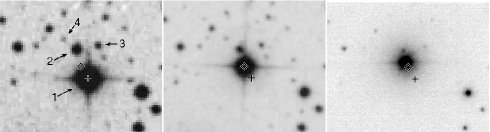
Figure 1.: The high proper motion ($0\hbox{$.\!\!^{\prime\prime}$}264$ yr^-1) of the transiting Neptune host-star HAT-P-11 (labeled as star 1) can be used to rule out the possibility that it is a blend with a background eclipsing binary. Images of a $2\hbox{${}^{\prime}$}\times 1\hbox{$.\mkern-4.0mu^{\prime}$}7$ field obtained in 1951, 1989 and 2007 (from left to right) show that there is no background object at the present location of HAT-P-11 that is within 8 magnitudes of HAT-P-11. This figure is taken from Bakos et al. 2009.

Like HAT-P-11b, HAT-P-26b is a transiting hot Neptune (Hartman et al. 2010b) for which the BS analysis was inconclusive. Again we leveraged the high proper motion of HAT-P-26 to rule out a blend with a background eclipsing binary, and used the version of blendanal described in Section 2 to reject the triple system blend scenario based on the photometry (Fig. 2).

Figure 2.: Results from using blendanal to model the transiting Neptune system HAT-P-26 as a hierarchical triple star system (left), a binary star where the fainter component has a transiting planet (center), and a binary star where the brighter component has a transiting planet (right). The mass of the brightest star in each case is fixed to $0.79~{}M_{\odot}$. We show $\chi^{2}$ as a function of the mass of the brighter EB component (left), and the fainter star (center and left). In each case points above the dashed line are rejected at the $3\sigma$ level. The triple star system is completely rejected. Binary star + planet scenarios that fit the photometry can be rejected based on the spectra of HAT-P-26.

3.2 Hot Saturns

The transiting hot Saturns HAT-P-12b (Hartman et al. 2009) and HAT-P-18b (Hartman et al. 2010a) are two cases where the BS appeared to correlate with the measured RVs suggesting that these might in fact be blends. We used blendanal to analyze both systems and concluded that neither could be modelled as a blend. For HAT-P-12 we used the high proper motion to rule out a blend with a background eclipsing binary, while for HAT-P-18 this scenario has also been ruled out with blendanal.

To understand the apparent correlation between the BS and RV for HAT-P-12 we estimated the effect of contamination from scattered moonlight on the BS measurements and found that much of the BS variation could be due to this effect. After correcting for the sky contamination, the BS and RV appeared to be uncorrelated. The tight relation between the expected BS due to sky contamination and the measured BS is particularly striking for HAT-P-18 and HAT-P-19 (Fig. 3).

Figure 3.: Bisector span (BS) vs. the expected BS due to scattered moonlight (sky contamination factor; SCF) for HAT-P-18 (left) and HAT-P-19 (right). In both cases there is a strong correlation between the measured and expected BS.

3.3 HTR294-001

Our last example is HTR294-001, a transit candidate which exhibits a striking BS variation that is in anti-phase with the RVs (Fig. 4). In addition to being in anti-phase, the BS semiamplitude is also an order of magnitude lower than the RV semiamplitude. Both of these factors indicate that the transiting object is most likely orbiting the brightest star in the system. We iteratively use blendanal to model the system as a hierarchical triple, and the TwO-Dimensional CORrelation (todcor; Mazeh & Zucker 1994) program to extract the RVs, and find that it is consistent with an F star that is transited by a very low-mass $0.075$–$0.085~{}M_{\odot}$ star, which is right at the stellar–brown dwarf transition, and blended with a K dwarf. The analysis of this intriguing system continues.

Figure 4.: Left: RVs for the transit candidate HTR294-001 measured from Keck/HIRES spectra obtained with an iodine cell and phased using the transit ephemeris. The solid line shows the best-fit orbit. Right: bisector spans (BS) for these same spectra. The BS are anti-correlated with the RVs and have an amplitude that is an order of magnitude lower than the RV amplitude. Iteratively applying blendanal to model the system as a blend, and todcor to measure the RVs leads to the conclusion that this is a hierarchical triple system.

• HATNet operations have been funded by NASA grants NNG04GN74G, NNX08AF23G and SAO IR&D grants. Work of G.Á.B. was supported by the Postdoctoral Fellowship of the NSF Astronomy and Astrophysics Program (AST-0702843).

References

Bakos, G. A., Noyes, R. W., Kovács, G., Stanek, K. Z., Sasselov, D. D., & Domsa, I. 2004, PASP, 116, 266

Bakos, G. Á., et al. 2010, 710, 1724

Etzel, P. B. 1981, NATO ASI, p. 111

Hartman, J. D., et al. 2009, ApJ, 706, 785

Hartman, J. D., et al. 2010a, ApJ submitted, arXiv:1007.4850

Hartman, J. D., et al. 2010b, ApJ submitted, arXiv:1010.1008

Kurtz, M. J., & Mink, D. J. 1998, PASP, 110, 934

Latham, D. W., et al. 2009, ApJ, 704, 1107

Mazeh, T., & Zucker, S. 1994, Ap&SS, 212, 349

Nelson, B., & Davis, W. D. 1972, ApJ, 174, 617

Pollacco, D. L., et al. 2006, PASP, 118, 1407

Popper, D. M., & Etzel, P. B. 1981, AJ, 86, 102

Queloz, D., et al. 2001, A&A, 379, 279

Torres, G., Konacki, M., Sasselov, D. D., & Jha, S. 2004, ApJ, 614, 979

Torres, G., Konacki, M., Sasselov, D. D., & Jha, S. 2005, ApJ, 619, 558

Torres, G., et al. 2007, ApJ, 666, L121

Torres, G., et al. 2010, ApJ, submitted, arXiv:1008.4393

Udalski, A., et al. 2002, Acta Astron., 52, 1