Memory-keeping effects and forgetfulness in the dynamics of a qubit coupled to a spin chain

Abstract

Using recently proposed measures for non-Markovianity [H. P. Breuer, E. M. Laine, and J. Piilo, Phys. Rev. Lett. 103, 210401 (2009)], we study the dynamics of a qubit coupled to a spin environment via an energy-exchange mechanism. We show the existence of a point, in the parameter space of the system, where the qubit dynamics is effectively Markovian and that such a point separates two regions with completely different dynamical behaviors. Indeed, our study demonstrates that the qubit evolution can in principle be tuned from a perfectly forgetful one to a deep non-Markovian regime where the qubit is strongly affected by the dynamical back-action of the environmental spins. By means of a theoretical quantum process tomography analysis, we provide a complete and intuitive characterization of the qubit channel.

In the study of open quantum systems, quite often the Markovian approximation has been a useful starting point to describe their dynamics. Only very recently, new and powerful tools have been designed in order to tackle the important question of explicitly quantifying the non-Markovian character of a system-environment interaction or a dynamical map breuer09 ; rivas09 ; wolf08 . Such a task is extremely important, given that non-Markovian effects are known or expected to occur in a wide range of physical situations, especially in the realm of solid-state devices where a system of interest is often exposed to memory-preserving environmental mechanisms. As a specific example, switching impurities have been shown to affect superconducting devices in various regimes martinis .

From a fundamental point of view, devising a reliable way to actually quantify non-Markovianity is very useful in light of the plethora of frequently ad hoc or technically rather involved approaches put forward so far in order to study memory-keeping environmental actions. A few instances emerge as promising measures for the non-Markovian nature. Wolf et al. wolf08 have proposed to quantify the degree of non-Markovianity of a map by considering the minimum amount of noise required in order to make the evolution of a system fully Markovian. On the other hand, in Ref. rivas09 , Rivas and co-investigators discussed two approaches, founded on the deviations of a given map from full divisibility. Finally, Breuer et al. proposed a way to quantify non-Markovian effects by looking at the back-action induced on the system under scrutiny by its memory-keeping environment breuer09 . Further approaches have been considered and measures have been proposed which are based on the use of other interesting instruments such as the quantum Fisher information sun09 .

In this paper, we focus on the non-Markovianity measure proposed in Ref. breuer09 to study the dynamics of a qubit coupled to a spin environment described by an $XY$ model in a transverse magnetic field. Our aim is to analyze a simple and yet non-trivial system-environment set, displaying a broad range of behaviors in the parameter space, in order to relate the features of the non-Markovianity measure to the known spectral and dynamical structures of the spin system. The choice of the model has been also dictated by the versatility demonstrated by spin-network systems in the engineering of protocols for short-range communication boseetal and also for the investigation of the interplay between quantum-statistical and quantum-information-related aspects rmp .

Intuitively, one would expect that the coupling to a spin environment always leads to a non-Markovian dynamics for the qubit. This can be justified by noticing that the environmental correlation time is non-zero even in the weak coupling regime and by conjecturing that, by increasing the coupling strength, a Markovian approximation can only become less valid. However, we demonstrate that this is not at all the case and that peculiar behaviors occur at intermediate couplings. The chosen measure for non-Markovianity, in fact, turns out to be identically null at specific dynamical regimes, thus demonstrating the absence of a net re-flux of information from the environment back to the qubit. Our study of non-Markovianity is thus novel and makes the use of measures for its quantification a valuable tool for the identification of special conditions in the parameter space of the environment. Moreover, our study opens up the possibility to exploit the different memory-keeping regimes induced by controlling and tuning the properties of the environment to effectively “drive” the qubit dynamics in a non-trivial and potentially very interesting way. The effective evolution of our two-level system could be guided across different regimes, ranging from strong environmental back-action to completely forgetful dynamics typical of a Markovian map. The potential of such flexibility for reliable control at the quantum level is a topic that will be explored in future.

The reminder of this paper is organized as follows. In Sec. I we introduce the model under scrutiny and revise the basic principles behind the chosen measure for non-Markovianity. We study a few cases amenable to a full analytical solution and highlight how, in a few of such instances, a simple experimental protocol can be designed for the inference of the properties of the qubit dynamics. Most importantly, we reveal the existence of an operating regime where the chosen measure is strictly null and relate such an effect to intriguing modifications occurring at the level of the energy spectrum of the qubit-environment system. Sec. II is devoted to the formal characterization of such peculiar point in the parameter space. We first demonstrate divisibility of the corresponding dynamical map, hence its Markovian nature, and then perform a theoretical analysis based on the use of quantum process tomography to quantitatively infer its properties. Finally, in Sec. III we draw our conclusions.

I The model and the measure

We consider a qubit $Q$ coupled to a chain $\Gamma$ of $N$ interacting spin-$1/2$ particles. The qubit is described by the spin-$1/2$ vector operator $\hat{\bm{s}}_{0}$, while the operator $\hat{\bm{s}}_{n}$ (${n{=}1,..,N}$) corresponds to the spin located at site $n$ of the chain $\Gamma$. The logical basis for the spins and $Q$ is given by $\{\left|0\right\rangle_{j},\left|1\right\rangle_{j}\}$ with $j=0,..,N$. The Hamiltonian ruling the intra-chain interaction is taken to be of the $XY$-Heisenberg type (we set $\hbar=1$)

$$\hat{\cal{H}}_{\Gamma}{=}-2\!\sum_{n=1}^{N-1}(J^{x}_{n}\hat{s}^{x}_{n}\hat{s}^{x}_{n+1}\!+\!J^{y}_{n}\hat{s}^{y}_{n}\hat{s}^{y}_{n+1})-2\sum_{n=1}^{N}h_{n}\hat{s}_{n}^{z},$$ (1)

where $h_{n}$ is the local field applied at site $n$. $\Gamma$ is open-ended with $J^{x,y}_{n}$’s and $h_{n}$’s being not necessarily uniform. The qubit is coupled to the first spin of the environment, embodied by $\Gamma$, via an exchange interaction of strengths $J^{x,y}_{0}$ and is subjected to a local field ${h}_{0}$ according to

$$\hat{\cal{H}}_{0}\!=\!-2(J^{x}_{0}\hat{s}^{x}_{0}\hat{s}^{x}_{1}+J^{y}_{0}\hat{s}^{y}_{0}\hat{s}^{y}_{1})\!-\!2h_{0}\hat{s}^{z}_{0}.$$ (2)

In order to determine the time-evolution of $Q$, we resort to the Heisenberg picture and the formal apparatus put forward in Refs. DiFrancoEtal07 , which provides particularly powerful tools for the study of the many-body problem embodied by $\hat{\cal H}_{0}+\hat{\cal H}_{\Gamma}$. Using the operator-expansion theorem and the algebra satisfied by Pauli matrices, we find that the time evolution of the components of ${\hat{\bm{s}}}_{0}$ reads

$$\hat{s}^{x}_{0}(t) =\frac{1}{2}\sum_{n=0}^{N}\left[\Pi^{x}_{n}(t)\hat{\sigma}^{x}_{n}+\Delta^{x}_{n}(t)\hat{\sigma}^{y}_{n}\right]\hat{P}_{n}~{},$$ (3)

$$\hat{s}^{y}_{0}(t) =\frac{1}{2}\sum_{n=0}^{N}\left[\Pi^{y}_{n}(t)\hat{\sigma}^{y}_{n}-\Delta^{y}_{n}(t)\hat{\sigma}^{x}_{n}\right]\hat{P}_{n}~{},$$

$$\hat{s}^{z}_{0}(t) =-i\hat{\sigma}^{x}_{0}(t)\hat{\sigma}^{y}_{0}(t)/2,$$

where $\hat{\sigma}_{n}^{\alpha}$ ($\alpha{=}x,y,z$) are the Pauli operators for the spin at site $n$ and $\hat{P}_{n}=\prod_{i=1}^{n-1}\hat{\sigma}^{z}_{i}$. The time-dependent coefficients $\Pi_{n}^{x}(t)$ and $\Delta_{n}^{x}(t)$ are the components of the $(N+1)$-dimensional vectors ${\bm{\Pi}}^{x}(t)$ and ${\bm{\Delta}}^{x}(t)$ defined by

$${\bm{\Pi}}^{x}(t) = \sum_{p=0}^{\infty}(-1)^{p}\frac{t^{2p}}{(2p)!}({\bm{\tau}}{\bm{\tau}}^{T})^{p}{\bm{v}},$$ (4)

$${\bm{\Delta}}^{x}(t) = \sum_{p=0}^{\infty}(-1)^{p}\frac{t^{2p+1}}{(2p+1)!}{\bm{\tau}^{T}}({\bm{\tau}}{\bm{\tau}}^{T})^{p}{\bm{v}},$$ (5)

where $T$ stands for transposition, the vector ${\bm{v}}$ has components $v_{i}=\delta_{i0}$ and the tri-diagonal adjacency matrix ${\bm{\tau}}$ has elements

$$\tau_{ij}=J_{i-1}^{x}\delta_{i-1,j}+J_{i}^{y}\delta_{i+1,j}-2h_{i}\delta_{i,j}.$$ (6)

Notice that we have labelled columns and rows of $(N{+}1){\times}(N{+}1)$ matrices and $(N{+}1)$-dimensional vectors using indices ranging from $0$ to $N$. The coefficients ${\bm{\Pi}}^{y}(t)$ and ${\bm{\Delta}}^{y}(t)$ are obtained from Eqs. (4) and (5) by replacing ${\bm{\tau}}$ with ${\bm{\tau}}^{T}$. Both $\bm{\tau\tau}^{T}$ and $\bm{\tau}^{T}\bm{\tau}$ can be easily diagonalized by orthogonal matrices ${\bf U}$ and ${\bf V}$ such that $({\bm{\tau}}{\bm{\tau}}^{T})^{p}{=}{\bf U}{\bm{\Lambda}}^{2p}{\bf U}^{T}$ and $({\bm{\tau}}^{T}{\bm{\tau}})^{p}{=}{\bf V}{\bm{\Lambda}}^{2p}{\bf V}^{T}$, with ${\bm{\Lambda}}$ a diagonal matrix whose elements $\lambda_{ij}=\lambda_{i}\delta_{ij}$ are the (positive) square roots of the eigenvalues of $\bm{\tau}^{T}\bm{\tau}$. Consequently, Eqs. (4) and (5) can be fully summed up to give

$${\bm{\Pi}}^{x}(t) ={\bm{U}}{\bm{\Omega}}(t){\bm{U}}^{T}{\bm{v}},~{}~{}{\bm{\Delta}}^{x}(t)={\bm{V}}{\bm{\Sigma}}(t){\bm{U}}^{T}{\bm{v}},$$ (7)

$${\bm{\Pi}}^{y}(t) ={\bm{V}}{\bm{\Omega}}(t){\bm{V}}^{T}{\bm{v}},~{}~{}{\bm{\Delta}}^{y}(t)={\bm{U}}{\bm{\Sigma}}(t){\bm{V}}^{T}{\bm{v}},$$

where ${\bm{\Omega}}(t)$ and ${\bm{\Sigma}}(t)$ are diagonal matrices with elements $\Omega_{ij}(t){=}\cos(\lambda_{i}t)\delta_{ij}$ and $\Sigma_{ij}(t){=}\sin(\lambda_{i}t)\delta_{ij}$.

By using Eqs. (3), one can determine the time evolution of the state of $Q$ as ${\rho}(t){=}\hat{\openone}/2{+}\sum_{\alpha}\langle\hat{s}^{\alpha}_{0}(t)\rangle\hat{\sigma}^{\alpha}_{0}$. In the evaluation of the expectation values required to determine $\rho(t)$ we assume that $Q$ and $\Gamma$ are initially uncorrelated. The conservation rule ${[\hat{\cal{H}},\bigotimes_{n=0}^{N}\hat{\sigma}^{z}_{n}]=0}$ and the property $\langle\hat{\sigma}_{n}^{\alpha}\hat{\sigma}_{m\neq n}^{\beta\neq\alpha}\rangle{=}0$ imply

$$\langle\hat{s}^{x}_{0}(t)\rangle{=}\frac{1}{2}\sum_{n=0}^{N}\left[\Pi^{x}_{n}(t)\langle\hat{P}_{n}\hat{\sigma}^{x}_{n}\rangle+\Delta^{x}_{n}(t)\langle\hat{P}_{n}\sigma^{y}_{n}\rangle\right],$$ (8)

$$\langle\hat{s}^{y}_{0}(t)\rangle{=}\frac{1}{2}\sum_{n=0}^{N}\left[\Pi^{y}_{n}(t)\langle\hat{P}_{n}\hat{\sigma}^{y}_{n}\rangle-\Delta^{y}_{n}(t)\langle\hat{P}_{n}\hat{\sigma}^{x}_{n}\rangle\right],$$

$$\langle\hat{s}^{z}_{0}(t)\rangle{=}\frac{1}{2}\sum_{n=0}^{N}\left[\Pi_{n}^{x}(t)\Pi_{n}^{y}(t)+\Delta_{n}^{x}(t)\Delta_{n}^{y}(t)\right]\langle\hat{\sigma}_{n}^{z}\rangle$$

$$- \frac{1}{2}\sum_{n<m}^{N}\left[\Pi_{n}^{y}(t)\Pi_{m}^{x}(t)+\Delta_{n}^{x}(t)\Delta_{m}^{y}(t)\right]\langle\hat{P}_{n+1}\hat{P}_{m}\hat{\sigma}_{n}^{x}\hat{\sigma}_{m}^{x}\rangle$$

$$- \frac{1}{2}\sum_{n<m}^{N}\left[\Pi_{n}^{x}(t)\Pi_{m}^{y}(t)+\Delta_{n}^{y}(t)\Delta_{m}^{x}(t)\right]\langle\hat{P}_{n+1}\hat{P}_{m}\hat{\sigma}_{n}^{y}\hat{\sigma}_{m}^{y}\rangle.$$

In order to evaluate the above equations one needs multi-spin correlation functions, involving, in particular, the degrees of freedom of $\Gamma$. To this end, we consider it to be in its ground state in what follows. However, as it will be shown later on, the value of the measure of non-Markovianity chosen for this work is independent of the state of $\Gamma$, provided that $\langle s^{x(y)}_{n}(0)\rangle=0$ holds, as it does for the ground state with no broken symmetry.

By using Eqs. (8), one can finally determine ${\rho}(t)$. The interaction with the spin chain acts for $Q$ as a dynamical map $\Phi(t,0)$ such that $\rho(t)=\Phi(t,0)\rho(0)$. The properties of the map depend on the relative weight of the various parameters entering $\hat{\cal H}_{0}{+}\hat{\cal H}_{\Gamma}$. Our aim is to characterize the non-Markovian nature of $\Phi$ as a function of these parameters.

To pursue our task, we consider the measure proposed in Ref. breuer09 , based on the study of the time-behavior of the trace distance ${\cal D}[{\rho}^{(1)}(t),{\rho}^{(2)}(t)]{=}\frac{1}{2}\text{Tr}|{\rho}^{(1)}(t){-}{\rho}^{(2)}(t)|{\in}[0,1]$ between two single-qubit density matrices ${\rho}^{(1,2)}(t)$. The trace distance is such that ${\cal D}[{\rho}^{(1)}(t),{\rho}^{(2)}(t)]{=}1$ when the two probed states are completely distinguishable, while it gives $0$ for identical states NC . The degree of non-Markovianity ${\cal N}(\Phi)$ of the dynamical map $\Phi$, is defined as

$${\cal N}(\Phi){=}\max\!\sum_{n}\{{\cal D}[{\rho^{(1)}(b_{n})},{\rho^{(2)}(b_{n})}]{-}{\cal D}[\rho^{(1)}(a_{n}),\rho^{(2)}(a_{n})]\}$$ (9)

where the maximization is performed over the states ${\rho^{(1,2)}(0)}$ and $(a_{n},b_{n})$ is the $n^{\text{th}}$ time window such that

$$\sigma[t,\rho^{(1,2)}(0)]=\partial_{t}{\cal D}[\rho^{(1)}(t),\rho^{(2)}(t)]>0.$$ (10)

The function $\sigma[t,\rho^{(1,2)}(0)]$, which has been dubbed flux of information in Ref. breuer09 , encompasses per se the condition for revealing non-Markovianity of an evolution: the mere existence of even a single region where $\sigma[t,\rho^{(1,2)}(0)]{>}0$ is sufficient to guarantee the non-Markovian nature. Conceptually, in fact, ${\cal N}(\Phi)$ accounts for all the temporal regions where the distance between two arbitrary input states increases, thus witnessing a re-flux of information from the environment to the system under scrutiny. Such re-flux of information amplifies the difference between two arbitrarily picked input states evolved up to the same instant of time. A Markovian dynamics is such that the above-mentioned re-flux never occurs and $\sigma[t,\rho^{(1,2)}(0)]<0$ always. For the case at hand and for two generic input density matrices $\rho^{(1,2)}(0)$, we find $D[{\rho}^{(1)}(t),{\rho}^{(2)}(t)]=\sqrt{\zeta}$, where

$$\zeta =\left[\Pi_{0}^{x}(t)\Pi_{0}^{y}(t)+\Delta_{0}^{x}(t)\Delta_{0}^{y}(t)\right]^{2}p^{2}$$ (11)

$$+\left|cf_{+}(\Pi_{0},\Delta_{0},t)+c^{*}f_{-}(\Pi_{0},\Delta_{0},t)\right|^{2}/{4}$$

with $f_{\pm}(\Pi_{0},\Delta_{0},t){=}\Pi_{0}^{x}(t)\pm\Pi_{0}^{y}(t){\pm}i\left[\Delta_{0}^{x}(t){\pm}\Delta_{0}^{y}(t)\right]$ where $p{=}\rho^{(1)}_{11}(0){-}\rho^{(2)}_{11}(0)$ and $c{=}\rho^{(1)}_{01}(0){-}\rho^{(2)}_{01}(0)$. We have used the notation $\rho^{(a)}_{ij}(0){=}{}_{0}\langle{i}|\rho^{(a)}\left|j\right\rangle_{0}$ with ${i,j}{=}0,1$ and $a{=}1,2$. It is worth noticing that in the above equation the initial state of the environment is completely absent, so that the environment’s multi-spin correlators are not relevant. Eq. (11) can be recast into a much more intuitive form by referring to the Bloch vectors $\textbf{r}_{a}{=}{(r^{x}_{a},r^{y}_{a},r^{z}_{a})}$ representative of the state $\rho^{(a)}$ (we have chosen $r^{\alpha}=\langle\hat{s}_{0}^{\alpha}\rangle$ as the mean value of the spin-${1}/{2}$ operator rather than that of the more usual Pauli operator to avoid the appearance of irrelevant ${1}/{2}$ factors). By calling $\Delta r^{\alpha}{=}r^{\alpha}_{1}{-}r^{\alpha}_{2}$ the difference between the vectors of two input states, we have

$$\zeta {=}\left|\textbf{r}_{1}(t){-}\textbf{r}_{2}\right(t)|^{2}{\equiv}[\Pi_{0}^{x}(t)\Pi_{0}^{y}(t){+}\Delta_{0}^{x}(t)\Delta_{0}^{y}(t)]^{2}\!\left(\Delta r^{z}\right)^{2}$$ (12)

$${+}[\Pi_{0}^{x}(t)\Delta r^{x}{+}\Delta_{0}^{x}(t)\Delta r^{y}]^{2}{+}[\Pi_{0}^{y}(t)\Delta r^{y}{-}\Delta_{0}^{y}(t)\Delta r^{x}]^{2}.$$

One can thus write the flux of information between the qubit and the environmental chain $\Gamma$ as

$$\sigma[t,\rho^{(1,2)}(0)]=\frac{\left(\Delta r^{z}\right)^{2}A\partial_{t}A+B\partial_{t}B+C\partial_{t}C}{{\cal D}[\rho^{(1)}(t),\rho^{(2)}(t)]},$$ (13)

where $A=\Pi_{0}^{x}(t)\Pi_{0}^{y}(t)+\Delta_{0}^{x}(t)\Delta_{0}^{y}(t)$, $B=\Pi_{0}^{x}(t)\Delta r^{x}+\Delta_{0}^{x}(t)\Delta r^{y}$, and $C=\Pi_{0}^{y}(t)\Delta r^{y}-\Delta_{0}^{y}(t)\Delta r^{x}$. Due to the non-negativity of ${{\cal D}[\rho^{(1)}(t),\rho^{(2)}(t)]}$, the condition for non-Markovian dynamics can be simply stated as $\left(\Delta r^{z}\right)^{2}{A\partial_{t}A+B\partial_{t}B+C\partial_{t}C}{>}0$. Numerically, it turns out that the maximum in the corresponding measure of non-Markovianity is achieved for $\rho^{(1,2)}(0)$ being antipodal pure states lying on the equatorial plane of $Q$’s Bloch sphere (we will come back to this point later in this paper). This considerably simplifies the necessary condition for memory-keeping dynamics to the form $\partial_{t}(B^{2}{+}C^{2}){>}0$.

Although our analysis can be carried out without major complications in the general case, in order to simplify the presentation, from now on we restrict ourselves to the case of a uniform spin environment with equal isotropic couplings between every pairs of nearest neighboring spins ($XX$-model) and set this coupling constant as our energy (and inverse time) unit. We thus consider $J_{0}^{x}{=}J_{0}^{y}{=}J_{0}$, a condition under which the measure of non-Markovianity becomes

$${\cal D}[{\rho}^{(1)}(t),{\rho}^{(2)}(t)]{=}\sqrt{(p^{2}f(t)+\left|c\right|^{2})f(t)},$$ (14)

where $f(t)=\Pi^{2}_{0}(t)+\Delta^{2}_{0}(t)\in[0,1]$. The corresponding rate of change of the trace distance is

$$\sigma[t,\rho^{(1,2)}(0)]=\frac{\left(2p^{2}f(t)+|c|^{2}\right)f^{\prime}(t)}{2{\cal D}[\rho^{(1)}(t),\rho^{(2)}(t)]}.$$ (15)

As $f(t){\geq}{0}$, the sign of $\sigma[t,\rho^{(1,2)}(0)]$ is determined by $f^{\prime}(t)$, regardless of the pair of input density matrices $\rho^{(1,2)}(0)$. Yet, we should look for the states maximizing the contributions to the trace distance within these time intervals. As $|f(t)|{\leq}1$, such optimization is achieved for $c{=}1$ and $p{=}0$; that is, antipodal pure states on the equatorial plane of the Bloch sphere, in line with the (more general) numerical findings reported above. The condition for non-Markovianity can be further elaborated as $f^{\prime}(t){=}2[\Pi_{0}(t)\Pi^{\prime}_{0}(t)+\Delta_{0}(t)\Delta^{\prime}_{0}(t)]{>}0$.

To pursue the task of evaluating ${\cal N}(\Phi)$ in the quite rich parameter space of our model, we start by considering the case of a qubit resonant with the spin environment, and assess the special case of $h_{0}{=}h$ first. It can be shown analytically that in this case one gets ${\Pi_{0}(t)={{\cal J}_{1}(2t)}\cos(2ht)}/{t}$ and ${\Delta_{0}(t)=-{{\cal J}_{1}(2t)}\sin(2ht)}/{t}$ ApollaroEtal10 , where ${\cal J}_{n}(x)$ is the Bessel function of order $n$ and argument $x$. Correspondingly, $f(t){=}{{\cal J}^{2}_{1}(2t)}/{t}^{2}$ and $f^{\prime}(t)=-{4{\cal J}_{1}(2t){\cal J}_{2}(2t)}/{t^{2}}$. For those states with $|c|=1$ and $p=0$ which maximize ${\cal N}$, we have the flux

$$\sigma[t,\rho^{(2,3)}(0)]=-(2/{t})\text{sgn}[{\cal J}_{1}(2t)]{\cal J}_{2}(2t)$$ (16)

with $\text{sgn}[x]$ being the sign function. Eq. (16) is independent of $h$, which is joint result of the condition $p=0$ and the invariance of the trace distance under the global unitary transformation embodied by the operator $\exp[{-ith\sum_{i=0}^{N}{\hat{\sigma}_{i}^{z}}}]$ needed in order to pass to the interaction picture. The time windows where $\sigma[t,\rho^{(1,2)}(0)]{>}0$ are determined by the chain-rule of the zeros of the Bessel functions. Overall, we get that the flux is positive for a time $t_{\sigma>0}{=}{\cup}(t^{1}_{i},t^{2}_{i})$ where $t^{1}_{i}$ ($t^{2}_{i}$) is the $i^{\text{th}}$ zero of the Bessel function of order 1 (2). From this special case and the general considerations reported above, we learn that ${\cal N}(\Phi)$ only depends on the detuning $\delta h=h-h_{0}$.

Due to this fact, the simple case in which all of the magnetic fields are absent ($h=h_{0}=0$), which can be tested experimentally in an easy way, allows to draw some interesting conclusions on the more general case $\delta h=0$. In absence of magnetic fields, indeed, the behavior of $\sigma$ and ${\cal N}$ can be extracted directly by monitoring the dynamics of the qubit. To show that this is indeed the case we start by noticing that, if $h/J=h_{0}/J=0$, we have $\Delta_{0}(t){=}0$ ApollaroEtal10 , so that both the trace distance and the flux of information are determined by $f(t)=\Pi^{2}_{0}(t)$, which represents the squared length of the Bloch vector, $|r(t)|^{2}$. This implies that, in order for $Q$ to experience a re-flux of information from $\Gamma$, $\Pi^{2}_{0}(t)$ has to be a strictly non-monotonic function. Therefore, we observe non-Markovian dynamics when the Bloch vector of the qubit is alternatively shrunk and elongated during its evolution. This can be witnessed by reconstructing the density matrix of $Q$ using standard quantum state tomography techniques statetomo ; NC , which are routinely implemented in a variety of physical setups. However, there is also an interesting alternative which does not require full state reconstruction. From the first of Eqs. (8), we get that $\langle\hat{s}_{0}^{x}(t)\rangle{=}\frac{1}{2}\Pi_{0}(t)\langle\hat{\sigma}_{0}^{x}(0)\rangle$. Thus, in the spirit of the proposals put forward in Refs. DiFrancoEtal07 ; DiFrancoEtal08 , by preparing the state of $Q$ in one of the eigenstates of $\hat{\sigma}^{x}_{0}$ [a choice that would be perfectly consistent with our results on the input states to be used for the calculation of ${\cal N}(\Phi)$] we can measure $\langle\hat{s}^{x}_{0}(t)\rangle$ to determine the non-Markovianity of the qubit dynamics, which would be revealed by its non-monotonic time behavior.

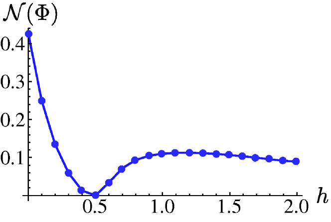
Figure 1: (Color online) ${\cal N}(\Phi)$ versus $h/J$ with $h_{0}/J=0$, $J_{0}/J=1$ and $N=100$. To avoid spurious recursion effects, the dynamics is evaluated up to a temporal cut-off of $\sim 2N/3$. We checked that the precise cut-off is not relevant and that the plot remains unchanged if $N$ is varied, provided $N\gg 1$. All quantities are dimensionless.

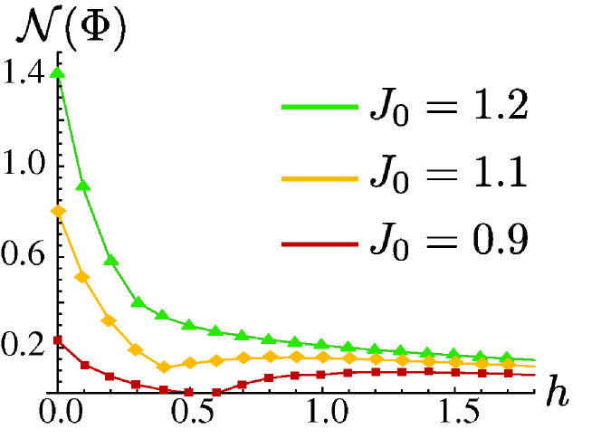
Figure 2: (Color online) ${\cal N}(\Phi)$ versus $h/J$ for $h_{0}/J=0$ and three different values of $J_{0}/J$ for a chain of $N=200$ spins. For $J_{0}/J{>}1$, the Markovianity point disappears. All quantities are dimensionless.

Other points in parameter space exist for which the model is amenable to an exact analytic solution. However, in order to give a complete overview of the behavior of ${\cal N}$, we first resort to numerical techniques to solve our model. The results of such an analysis are shown in Fig. 1, where the quantitative degree of non-Markovianity is shown as a function of $h/J$ (we set $h_{0}{=}0$) in the isotropic case and for equal intra-chain and qubit-environment coupling strengths.

A highly non-trivial behavior followed by ${\cal N}(\Phi)$ is revealed. The largest deviation from a Markovian dynamics is achieved at $h/J=0$ while, for $0\leq h/J\leq 0.5$, ${\cal N}(\Phi)$ decreases monotonically to zero. By further increasing $h$ we see that ${\cal N}(\Phi)$ achieves a very broad maximum around the saturation point $h/J\simeq{1}$ of the environmental chain. Finally, it goes to zero for $h/J\gg 1$, as it should be expected given that this situation corresponds to an effective decoupling of the qubit from the environment ApollaroEtal10 . By generalizing our study to the case of $h_{0}/J\neq{0}$, we emphasize the presence of a Markovianity point at $\delta{h}/J{=}1/2$. It turns out that this point separates two regions in which the dynamics of the qubit (although being non-Markovian in both cases) is completely different. For $\delta h/J{\leq}1/2$, indeed, the qubit tends toward a unique equilibrium state at long times, irrespective of the initial condition; that is, the trace distance goes to zero after some oscillations. For larger detunings, on the other hand, the trace distance does not decay to zero, implying that some information about the initial state (and in particular, about the relative phase between its two components) is trapped in the qubit.

The Markovianity point at $\delta h/J{=}{1}/{2}$ (with $J_{0}/J{=}1$) is one of those points in parameter space for which the model can be treated fully analytically yueh04 . We have $\Pi_{0}(t){=}{\cal J}_{0}(2t)\cos t{+}{\cal J}_{1}(2t)\sin t$ and $\Delta_{0}(t){=}{\cal J}_{1}(2t)\cos t{-}{\cal J}_{0}(2t)\sin t$ ApollaroEtal10 , so $f(t){=}{\cal J}_{0}^{2}(2t){+}{\cal J}_{1}^{2}(2t)$ and $f^{\prime}(t){=}{-}{2{\cal J}_{1}^{2}(2t)}/{t}{<}0~{}\forall{t}$. As a consequence, the corresponding non-Markovianity measure is always zero at this point of the parameter space, which is a very interesting result due to the relatively large $Q-\Gamma$ coupling strength. Such a feature, in fact, would intuitively lead to exclude any possibility of a forgetful dynamics undergone by the qubit. Yet, this is not the case and a fully Markovian evolution is in order under these working conditions. A deeper characterization of this Markovian dynamical map is given in Sec. II.

As $J_{0}$ represents the energy scale of the qubit-environment interaction, it is natural to expect that significant changes in ${\cal N}(\Phi)$ occur as this parameter varies. In particular, we find that i) a Markovianity point with ${\cal N}(\Phi){=}0$ only exists for $J_{0}/J{\leq}1$ and ii) ${\cal N}(\Phi)$ tends progressively towards a monotonically decreasing function of $\delta h$ if $J_{0}/J$ grows from $1$ to $\sqrt{2}$ [see Fig. 2]. Strikingly, at $J_{0}/J{=}\sqrt{2}$ and $\delta h{=}0$, the adopted measure of non-Markovianity diverges, as it can be checked by using the analytic integrability of the qubit-chain interaction at this point in the parameter space. Indeed, at $J_{0}/J{=}\sqrt{2}$, we have $\Pi_{0}(t)={\cal J}_{0}(2t)$ and $\sigma(t){=}-2\text{sgn}[{\cal J}_{0}(2t)]{\cal J}_{1}(2t)$. Integrating over all the positive time intervals determined by means of the usual chain rule we get ${\cal N}(\Phi){\rightarrow}\infty$, thus witnessing a strong back-action of $\Gamma$ on the state of the qubit. The divergence of ${\cal N}(\Phi)$ should not surprise as it is common to other situations with spin-environments, such as the so-called central-spin model where a single qubit is simultaneously coupled to $N$ independent environmental spins via Ising-like interactions (see Breuer et al. in Ref. breuer09 ). We provide a physical explanation for the enhanced non-Markovian nature of the qubit dynamics simply by looking at the spectrum of the Hamiltonian ruling the evolution of the qubit-chain system. For $J_{0}/J{\geq}\sqrt{2}$, the spectrum of $\hat{\cal H}_{\Gamma}+\hat{\cal H}_{0}$ exhibits a continuous spectrum (a band of extended eigenstates) that is lower- and upper-bounded by two discrete energy levels whose eigenstates are localized at the sites occupied by the qubit and the first spin of $\Gamma$ nota . As a consequence, a certain amount of information remains trapped into such a localized state, bouncing back and forth between the qubit and the first spin and therefore mimicking a highly non-Markovian dynamics characterized by strong back-action, so that ${\cal N}(\Phi)$ diverges.

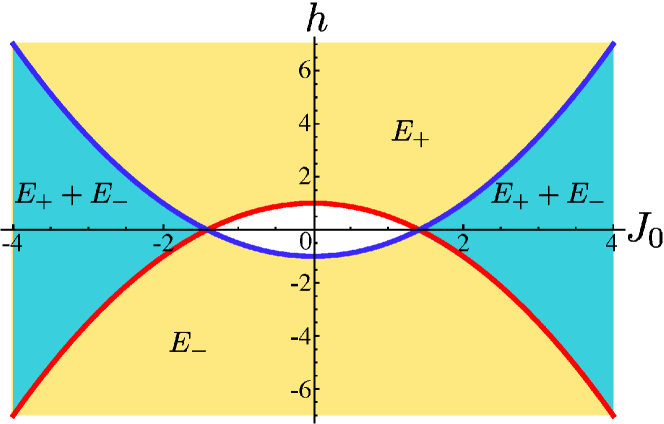
Figure 3: (Color online) We call $E_{+}$ ($E_{-}$) a discrete level lying above (below) the continuous energy band in the (single particle) spectrum of the total Hamiltonian $\hat{\cal H}_{0}+\hat{\cal H}_{\Gamma}$. The parabolae $h/J=\pm[1-(J_{0}/J)^{2}/2]$ divide the $(h/J,J_{0}/J)$ parameter plane in three regions with one, two and no localized state (light-colored, dark-colored and uncolored region in the plane, respectively). All quantities are dimensionless.

An analysis similar to the one performed just above allows us to obtain an intuition for the behavior of the measure of non-Markovianity near this point. For $\delta h/J{>}{1}/{2}$ the spectrum of the system shows one eigenenergy out of the band and its corresponding eigenvector is localized around the site occupied by $Q$. This can explain the information trapping that occurs for $\delta h/J{>}1/2$. For definiteness, in what follows we report explicit results for the case $h_{0}/J=0$. Therefore, from now on, we consider $\delta h/J\equiv h/J$.

In order to determine the existence of a more general connection between the emergence of localized eigenstates in the system-environment spectrum and a point of zero-${\cal N}$ in the qubit evolution, we analyze the $(h,J_{0})$-plane to find out where localized eigenstates appear and then evaluate the corresponding degree of non-Markovianity. In doing this, we take advantage of the fact that the Hamiltonian describing an environmental $XX$-model has the same single-particle energy spectrum as a tight-binding model with an impurity. Following the approach given in Ref. pury91 , we deduce that, in the $(h/J,J_{0}/J)$ plane, the parabolae $h/J=\pm[1-(J_{0}/J)^{2}/{2}]$ define regions with respectively zero, one and two localized energy levels out of a continuous-energy band (see Fig. 3).

The central region with no localized energy state and the zones with only one localized state (either a upper-lying or lower-lying one with respect to the continuous band) correspond to ${\cal N}(\Phi)\neq 0$, although finite. The frontiers of such regions, marked by the parabolae, give the limiting values of $(h/J,J_{0}/J)$ for the appearance of the localized states and are such that ${\cal N}(\Phi)=0$ only for $J_{0}/J\leq 1$, whereas for $1<J_{0}/J<\sqrt{2}$ the measure of non-Markovianity is non-null and finite. Finally, the regions with two localized states and their frontier with the no-localized state region have ${\cal N}(\Phi){\rightarrow}\infty$, in line with the analytical results discussed above.

In particular, we remark once again that the Markovianity points (when they exist, i.e. for $J_{0}/J\leq 1$) stay on the parabolae; that is, they are found to occur at the onset for the existence of one discrete eigenstate outside the energy band. This kind of state contains a spatially localized spin excitation with a localization length that decreases with increasing $h$ nota . Precisely at the border, the localization length becomes as large as the length of the chain itself, so that all of the environmental spins are involved in (or share excitation of) the initial state. This can intuitively justify the fact that ${\cal N}$ is zero there. For $J_{0}/J>1$, on the other hand, the first spin of the environment becomes more important for the dynamics of the qubit (which is “strongly coupled” to it) and an information exchange is always found to occur between them, irrespectively of the existence of the discrete level. This information re-flux becomes more and more pronounced with increasing $J_{0}/J$ and decreasing $h/J$.

To stress once more the close relationship between the non-Markovianity measure and the properties of the overall Hamiltonian $\hat{\cal{H}}_{\Gamma}+\hat{\cal{H}}_{0}$, we report here the energy distribution of the excitations which are present in the initial state of the system (given by the product of an equatorial state for the qubit times the ground state of the environment). These excitations are spin-less fermions of the Jordan-Wigner type and the procedure to obtain them is the one described, e.g., in Ref. apollaro08 . Fig. 4 reports the average value of the excitation number in the initial state vs single-particle-energy for various values of the magnetic field. The plot shows what happens near a Markovianity point: the energy distribution of initial-state excitations becomes flat (i.e., structure-less) at the ${\cal N}=0$ point, while it shows a maximum for lower values of $h$, corresponding to a finite value of ${\cal N}$, and a spike for $h/J>0.5$, corresponding to the discrete level giving rise to information trapping.

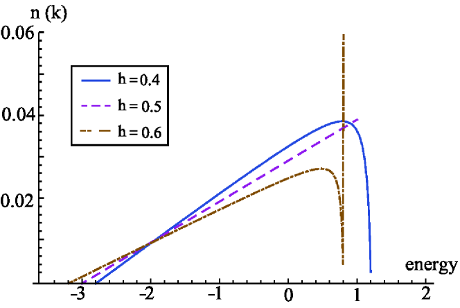
Figure 4: (Color online) Average number of fermion excitations in the initial state for a qubit-chain system with $N+1=50$, coupling strength $J_{0}/J=1$ and three values of magnetic field around the Markovianity point $(h/J=0.5,h_{0}/J=0)$. The initial state is always taken to be the tensor product of an equatorial state of $Q$ and the ground state of $\Gamma$.

From this discussion we conclude that the measure of non-Markovianity of the qubit dynamics is in fact a detector of general aspects of the full qubit+environment system and that various features of ${\cal N}(\Phi)$ can be related to general characteristics of the overall many-body problem described by the full Hamiltonian model.

II Characterization of the point of zero-measure

The occurrence of a null value of ${\cal N}(\Phi)$ at $h/J=1/2$ and $J_{0}/J=1$ deserves a special attention. Naively, one could expect a special behavior to occur at the chain saturation point (i.e. at $h/J=1$), where the intrinsic properties of the environmental system are markedly different from the situation at $h/J<1$. To the best of our knowledge, indeed, no significant dynamical feature has been reported for the model under scrutiny away from saturation.

II.1 Characterization of the dynamical map: formal features and divisibility

The aim of this Section is to characterize the dynamical map that we obtained for the qubit under these conditions.

(a)                                   (b)   

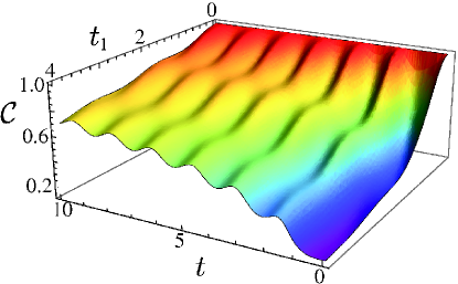
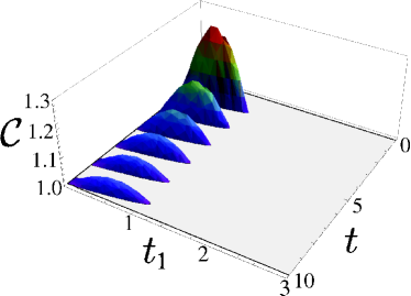
Figure 5: (Color online) Divisibility condition ${\cal C}$ against $t$ and $t_{1}$ for qubit $Q$ initially prepared in $(\left|0\right\rangle_{0}+\left|1\right\rangle_{0})/\sqrt{2}$. Divisibility is guaranteed for $0\leq{\cal C}\leq{1}$. In panel (a) we have taken $J_{0}/J=1$ with $h_{0}/J=h/J=1/2$, while in (b) it is $h/J=1.1$. All quantities are dimensionless.

Thanks to the analytical solution for the case at hand provided in Ref. yueh04 , we can sum up the terms appearing in Eq. (8) and determine the complete density matrix of $Q$. For $n=0,..,N$ we have

$$\Pi_{n}(t){=}\begin{cases}(-1)^{\frac{n}{2}}[\sin(t){\cal J}_{n+1}(2t){+}\cos(t){\cal J}_{n}(2t)]&\text{$n$ even},\\ (-1)^{\frac{n+1}{2}}[\cos(t){\cal J}_{n+1}(2t){-}\sin(t){\cal J}_{n}(2t)]&\text{$n$ odd}\end{cases}$$ (17)

and

$$\Delta_{n}(t){=}\begin{cases}(-1)^{\frac{n}{2}}[\cos(t){\cal J}_{n+1}(2t){-}\sin(t){\cal J}_{n}(2t)]&\!\text{$n$ even},\\ (-1)^{\frac{n+3}{2}}[\sin(t){\cal J}_{n+1}(2t){+}\cos(t){\cal J}_{n}(2t)]&\text{$n$ odd}.\end{cases}$$ (18)

The dynamical map transforms the elements of the input density matrix $\rho_{ij}(0)~{}(i,j=0,1)$ as

$$\rho_{00}(t) =f(t)\rho_{00}(0)+A_{00}^{11}(t),~{}~{}\rho_{01}(t) =A_{01}^{01}(t)\rho_{01}(0),$$ (19)

$$\rho_{11}(t) =A_{11}^{00}(t)+f(t)\rho_{11}(0),~{}~{}\rho_{10}(t) =A_{10}^{10}(t)\rho_{10}(0),$$

with $A_{00}^{11}(t){=}[1{-}f(t){+}g(t)]/{2}$, $A_{11}^{00}(t){=}[1{-}f(t){-}g(t)]/{2}$ and $A_{01}^{01}(t){=}\Pi_{0}(t){+}i\Delta_{0}(t){=}[A_{10}^{10}(t)]^{*}$, and where $f(t){=}\Pi_{0}(t)^{2}{+}\Delta_{0}(t)^{2}$ has already been defined in Sec. I. We introduced here the function $g(t)=\sum_{n=1}^{N}[\Pi^{2}_{n}(t)+\Delta^{2}_{n}(t)]\langle\hat{\sigma}^{z}_{n}\rangle-\frac{1}{4}\sum_{\begin{subarray}{c}n\neq{m}=1\end{subarray}}^{N}[\Pi_{n}(t)\Pi_{m}(t)+\Delta_{n}(t)\Delta_{m}(t)]g_{nm}$, written in terms of the magnetization and the two-point longitudinal correlation function

$$\langle\hat{\sigma}_{n}^{z}\rangle {=}1{-}\frac{2}{N+1}\left(k_{F}-\frac{\cos[(k_{F}+1)\vartheta_{n}]\sin[k_{F}\vartheta_{n}]}{\sin\vartheta_{n}}\right),$$ (20)

$$g_{nm} {\equiv}\langle\hat{P}_{n}\hat{P}_{m}\hat{\sigma}_{n}^{x}\hat{\sigma}_{m}^{x}\rangle=\frac{\varphi_{n,k_{F}+1}\varphi_{m,k_{F}}-\varphi_{n,k_{F}}\varphi_{m,k_{F}+1}}{2\left(\cos\vartheta_{n}-\cos\vartheta_{m}\right)},$$

with $\varphi_{j,k}{=}\sqrt{{2}/{(N+1)}}\sin(j\vartheta_{k})$, ${\vartheta_{k}={k\pi}/({N+1})}$, ${k=1,..,N}$ and $k_{F}$ being the Fermi wave number, see Ref. wonmin .

The condition for divisibility stated in Ref. breuer09 implies the existence of a completely positive dynamical map $\Psi(t+t_{1},t)$ such that, for two arbitrary instants of time $t$ and $t_{1}$, we have ${\Phi}(t+t_{1},0)={\Psi}(t+t_{1},t){\Phi}(t,0)$. Here $\Phi(t,0)$ is the dynamical map in Eq. (19). Any dynamical map that is divisible according to the above definition is Markovian. This implies that non-divisibility is a necessary condition for memory-keeping effects in the evolution of a system. A dynamical connection $\Psi(t+t_{1},t)$ between the states ${\Phi}(t+t_{1},0)\rho(0)$ and ${\Phi}(t,0)\rho(0)$ can be straightforwardly found to be given by the map changing the elements of the qubit state $\rho(t)$ at time $t$ into

$$\rho_{00}(t+t_{1}) {=}\frac{f(t+t_{1})}{f(t)}\rho_{00}(t){+}A_{00}^{11}(t+t_{1}){-}\frac{f(t+t_{1})}{f(t)}A_{00}^{11}(t),$$ (21)

$$\rho_{11}(t+t_{1}) {=}\frac{f(t+t_{1})}{f(t)}\rho_{11}(t){+}A_{11}^{00}(t+t_{1}){-}\frac{f(t+t_{1})}{f(t)}A_{11}^{00}(t),$$

$$\rho_{01}(t+t_{1}) {=}\rho^{*}_{10}(t+t_{1})=\frac{A_{01}^{01}(t+t_{1})}{A_{01}^{01}(t)}\rho_{01}(t).$$

Therefore, in order to ensure the divisibility of $\Phi(t+t_{1},0)$, we should investigate the complete positivity of $\Psi(t+t_{1},t)$. To this purpose we make use of the Choi-Jamiolkowski isomorphism CJ and prove the complete positivity of $\Psi(t+t_{1},t)$ by checking the non-negativity of $\left(\Psi(t+t_{1},t)\otimes\mathbf{I}_{2}\right)\rho$, where $\rho$ is the density matrix of one of the Bell states ruskai and $\mathbf{I}_{2}$ is the identity map. By choosing $\rho(t){=}\frac{1}{2}\left(\left|00\right\rangle+\left|11\right\rangle\right)\left(\left\langle 00\right|+\left\langle 11\right|\right)$, the action of the map $\left(\Psi(t+t_{1},t)\otimes\mathbf{I}_{2}\right)$ determines the following non-zero matrix elements (up to an irrelevant factor ${1}/{2}$) at time $t+t_{1}$

$$\rho_{00,00}(t+t_{1},t){=}\frac{f(t+t_{1})}{f(t)}{+}A_{00}^{11}(t+t_{1}){-}\frac{f(t+t_{1})}{f(t)}A_{00}^{11}(t),$$ (22)

$$\rho_{00,11}(t+t_{1},t){=}A_{00}^{11}(t+t_{1}){-}\frac{f(t+t_{1})}{f(t)}A_{00}^{11}(t),$$

$$\rho_{11,00}(t+t_{1},t){=}A_{11}^{00}(t+t_{1}){-}\frac{f(t+t_{1})}{f(t)}A_{11}^{00}(t),$$

$$\rho_{11,11}(t+t_{1},t){=}\frac{f(t+t_{1})}{f(t)}{+}A_{11}^{00}(t+t_{1}){-}\frac{f(t+t_{1})}{f(t)}A_{11}^{00}(t),$$

$$\rho_{01,01}(t+t_{1},t){=}\rho^{*}_{01,01}(t+t_{1},t)=\frac{A_{01}^{01}(t+t_{1})}{A_{01}^{01}(t)}.$$

Here, we have used $\rho_{i^{\prime}j^{\prime},ij}{=}\left\langle i^{\prime}i\right|\rho\left|j^{\prime}j\right\rangle$ with the primed (unprimed) indeces corresponding to the evolving (non-evolving) qubit. The condition for positivity of the composite two-qubit map turns out to be equivalent to the positivity condition of the single-qubit one given in Eqs. (21), which is in turn translated into the inequality ${0\leq{\cal C}(t,t_{1})\leq{1}}$ with

$${\cal C}(t,t_{1})=4|\rho_{01}(t+t_{1})|^{2}+[\rho_{00}(t+t_{1})-\rho_{11}(t+t_{1})]^{2}.$$ (23)

In Fig. 5 we show the typical behavior of ${\cal C}(t,t_{1})$ at the Markovianity point [panel (a)] and away from it [panel (b)]. We have taken the qubit $Q$ as prepared in $(\left|0\right\rangle_{0}+\left|1\right\rangle_{0})/\sqrt{2}$, which is a significant case as equatorial states in the Bloch sphere are those optimizing the calculation of ${\cal N}(\Phi)$. Although this is simply a representative case, we have checked that for a uniform distribution of random initial states of $Q$, no significant quantitative deviations from the picture drawn here are observed. Clearly, by moving away from $h/J{=}1/2$, temporal regions where ${\cal C}(t,t_{1}){>}1$ are achieved. This demonstrates, from a slightly different perspective, the flexibility of the effective qubit evolution: a wide range of dynamical situations is spanned, from fully forgetful to deeply non-Markovian dynamics, strongly affected by the environmental back-action. The kind of evolution of $Q$ can be determined by tuning the parameters of the environment and its interaction with it.

II.2 Formal characterization of the channel through theoretical quantum process tomography

We now turn our attention towards the formal characterization of the channel achieved at the Markovianity point, so as to qualitatively explain the reasons behind the nature of the corresponding qubit evolution. We stress that this sort of investigation is meaningful only at this specific point in parameter space, where complete positivity is guaranteed. In principle, full information on the reduced dynamics of $Q$ could be gathered from the Kraus operators $\{\hat{K}_{i}\}$ such that $\Phi(t,0)\rho{\equiv}\sum_{i}\hat{K}_{i}\varrho\hat{K}^{\dagger}_{i}$ with $\rho$ the density matrix of the generic qubit and $\sum_{i}\hat{K}_{i}^{{\dagger}}\hat{K}_{i}{=}\hat{\openone}$. As their direct computation is not possible due to the complications of the $Q-\Gamma$ coupling, here we gain useful information on the structure of the $\hat{K}_{i}$’s by means of the formal apparatus for quantum process tomography NC , that we briefly remind here.

The characterization of a dynamical map ${\Phi}$ reduces to the determination of a complete set of orthogonal operators $\{\hat{\cal K}_{m}\}$ over which one can perform the decomposition $\hat{K}_{i}{=}\sum_{m}{e}_{im}\hat{\cal K}_{m}$ so as to get

$${\Phi}(t,0)\varrho=\sum_{m,n}\chi_{mn}\hat{\cal K}_{m}\varrho\hat{\cal K}^{\dagger}_{n},$$ (24)

where the channel matrix $\chi_{mn}{=}\sum_{i}e_{im}e^{*}_{in}$ has been introduced. This is a pragmatically very useful result as it shows that it is sufficient to consider a fixed set of operators, whose knowledge is enough to characterize a channel through the matrix $\chi$. The action of $\Phi$ over a generic element $\left|n\right\rangle\!\left\langle m\right|$ of a basis in the space of the $2{\times}{2}$ matrices (with $n,m{=}0,1$) can be determined from a knowledge of the map ${\Phi}$ on the fixed set of states $\left|0\right\rangle,\left|1\right\rangle,\left|+\right\rangle{=}(1/\sqrt{2})(\left|0\right\rangle{+}\left|1\right\rangle)$ and $\left|+_{y}\right\rangle{=}(1/\sqrt{2})(\left|0\right\rangle{+}i\left|1\right\rangle)$ as follows

$${\cal E}(\left|n\right\rangle\left\langle m\right|) ={\cal E}(\left|+\right\rangle\left\langle+\right|)+i{\cal E}(\left|+_{y}\right\rangle\left\langle+_{y}\right|)$$ (25)

$$-\frac{i+1}{2}[{\cal E}(\left|n\right\rangle\left\langle n\right|)+{\cal E}(\left|m\right\rangle\left\langle m\right|)].$$

Therefore, each $\varrho_{j}=\left|n\right\rangle\left\langle m\right|$ (with $j=1,..,4$) can be found completely via state tomography of just four fixed states. Clearly, ${\Phi}(\varrho_{j})=\sum_{k}\lambda_{jk}\varrho_{k}$ as $\{\varrho_{k}\}$ form a basis. From the above discussion we have

$${\Phi}(t,0)\varrho_{j}{=}\sum_{m,n}\hat{\cal K}_{m}\varrho_{j}\hat{\cal K}^{{\dagger}}_{n}\chi_{mn}{=}\sum_{m,n,k}\beta^{mn}_{jk}\varrho_{k}\chi_{mn}{=}\sum_{k}\lambda_{jk}\varrho_{k},$$ (26)

where we have defined $\hat{\cal K}_{m}\varrho_{j}\hat{\cal K}^{\dagger}_{n}=\sum_{k}\beta^{mn}_{jk}\varrho_{k}$ so that we can write

$${\lambda_{jk}=\sum_{m,n}\beta^{mn}_{jk}\chi_{mn}}.$$ (27)

The complex tensor $\beta^{mn}_{jk}$ is set once we make a choice for $\{\hat{{\cal K}}_{i}\}$ and the $\lambda_{jk}$’s are determined from a knowledge of ${\Phi}(\varrho_{j})$. By inverting Eq. (27), we can determine the channel matrix $\chi$ and characterize the map. Let $\hat{\cal U}^{\dagger}$ be the operator diagonalizing the channel matrix. It is straightforward to prove that, if $D_{i}$ are the elements of the diagonal matrix $\hat{\cal U}^{\dagger}\chi{\hat{\cal U}}$, then $e_{im}=\sqrt{D_{i}}\hat{U}_{mi}$ so that

$$\hat{K}_{i}=\sqrt{D_{i}}\sum_{j}\hat{\cal U}_{ji}\hat{\cal K}_{j}.$$ (28)

This apparatus can be applied to the problem at hand. To this end, we numerically determine the evolution of the four qubit states $\left|0\right\rangle$, $\left|1\right\rangle$, $\left|+\right\rangle$ and $\left|+_{y}\right\rangle$ at $h/J{=}1/2$, $h_{0}{=}0$ and in the uniform-coupling case for $N{+}1{=}150$. As the time-scale within which an excitation travels back and forth to $Q$ scales as $N$ ApollaroEtal10 , in order to avoid recurrence effects we limit the time-window of our analysis to $[0,2N/3]{=}[0,100]$, which we chop into small intervals of amplitude $0.2$. At each instant of time in such a temporal partition, we evaluate the evolution of the four probing states given above. This is the basis for the reconstruction of the Kraus operators, which is performed as described above. The results of our numerical calculations are four Kraus operators, whose form depends on the instant of time at which the dynamics is evaluated. In principle, an analytic form of such operators can be given. Upon inspection, one can see that the action of the channel embodied by $\Gamma$ over the four probing qubit states can be summarized as follows

$$\left|0\right\rangle{\rightarrow}\varrho_{0}{=}\begin{pmatrix}\alpha&0\\ 0&1-\alpha\end{pmatrix},\left|+\right\rangle{\rightarrow}\varrho_{+}{=}\begin{pmatrix}a&b+ic\\ b-ic&1-a\end{pmatrix},$$ (29)

$$\left|1\right\rangle{\rightarrow}\varrho_{1}{=}\begin{pmatrix}\beta&0\\ 0&1-\beta\end{pmatrix}\!,\left|+_{y}\right\rangle{\rightarrow}\varrho_{+_{y}}{=}\begin{pmatrix}a&-c-ib\\ -c+ib&1-a\end{pmatrix}$$

with $a,\alpha,\beta\in[0,1]$ and $b,c\in\mathbb{C}$. The form of the corresponding analytical Kraus operator can then be found, although their cumbersome nature makes them unsuitable to be reported here. Despite the lack of analytic formulae, useful information can be gathered from this study. Fig. 6 shows the dynamics of 10 random pure input states of the qubit. Each dot represents the state of the qubit at time $t$ in the space of the density matrices. Colors identify the evolved states of a given input one. As time increases, i.e. as we follow the points of the same color from the outer to the inner region of the plot, the Bloch vector of each initial pure state spirals converging towards the center. That is, the state becomes close to a maximally mixed state.

We should mention that, for any fixed $N$, this does not exactly occur as the final state of $Q$ lies slightly off-set along the $z$-axis and does not describe a perfect statistical mixture. We ascribe such an off-set to the finite length of the chain being studied and the existence of a sort of effective magnetic field (scaling as $1/N$) acting on $Q$ and induced by its coupling with the environmental chain, which determines the residual polarization of the qubit. Numerical evidences suggest that, in the thermodynamical limit, such a residual polarization effectively disappears and the final state of the evolution is $\openone/2$.

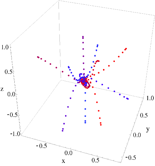
Figure 6: (Color online) Dynamics of $10$ random pure initial states of qubit $Q$ pictured in the Bloch sphere. Each dot shows the qubit state (evolved from the corresponding input state) at a given instant of time. Different colors stand for different initial states. Time increases as the dots move towards point $(0,0,0)$, thus showing that $Q$ converges towards a state close to a fully mixed one.

As discussed in the previous Section, from the study of the trace distance ${\cal D}[\rho^{(1)}(t),\rho^{(2)}(t)]$ at the basis of our chosen measure of non-Markovianity, one can infer an interesting general trend: for values of $h/J\leq 1/2$, ${\cal D}$ generally tends to zero at long evolution times. In order to put such an effect in context, here we study the long-time distribution of density matrices resulting from the evolution of a large sample of random input states according to the channel identified through quantum process tomography. Fig. 7 (a) shows the agreement between the effective description provided here and the true physical effect induced on the state of $Q$ by $\Gamma$.

(a)                                   (b)

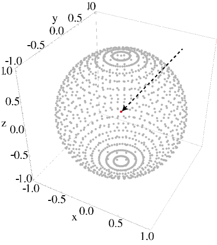
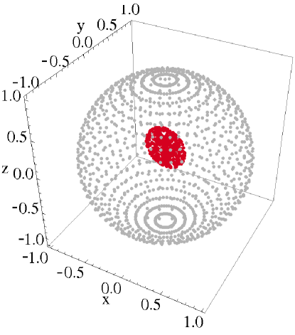
Figure 7: (Color online) (a) Distribution of density matrices evolved according to the dynamics induced by a quantum channel corresponding to $h/J=1/2$. We consider a sample of $500$ random initial states. Regardless of the initial density matrix, the final state is the same, thus resulting in a zero-volume state distribution. This is no longer the case for $h/J=0.6$ [panel (b)], where a finite-volume distribution of final states is found.

The red dot close to the center of the sphere shows the ensemble of $500$ random input states evolved until a final time equal to $100$. Clearly, there is a single fixed point of the map towards which any input state converges after a sufficient amount of time.

As anticipated, by repeating the above analysis for $h/J{>}1/2$, we get a distribution of long-time evolved output states which is much more widespread, even at very small deviations from the Markovian case. An example is given in Fig. 7 (b) for $h/J{=}0.6$. At long interaction times, the channel does not bring its input states to the same unique state, but a finite-dimensional subspace of asymptotic states exists.

Going back to our attempt of describing the dynamics as an effective channel, we have considered the case of a qubit evolving under a Markovian channel resulting from the action of a generalized amplitude damping channel and an independent dephasing mechanism. The output state for such a process can be written as

$$\rho(t)=\begin{pmatrix}\rho_{00}(0)e^{-2\tilde{\gamma}(2\tilde{\mu}+1)t}+\frac{\tilde{\mu}+1}{2\tilde{\mu}+1}[1-e^{-2\tilde{\gamma}(2\tilde{\mu}+1)t}]&\rho_{01}(0)e^{-[2\tilde{\Gamma}+\tilde{\gamma}(2\tilde{\mu}+1)]t}\\ \rho_{10}(0)e^{-[2\tilde{\Gamma}+\tilde{\gamma}(2\tilde{\mu}+1)]t}&\frac{\tilde{\mu}}{2\tilde{\mu}+1}+[\frac{\tilde{\mu}+1}{2\tilde{\mu}+1}-\rho_{00}(0)]e^{-2\tilde{\gamma}(2\tilde{\mu}+1)t}\end{pmatrix}$$ (30)

with $\tilde{\mu}$ being the mean occupation number of the thermal environment responsible for the generalized amplitude damping, $\tilde{\gamma}$ the rate of amplitude damping and $\tilde{\Gamma}$ the rate of dephasing. From this expression, one can determine the matrix of the corresponding process, to be compared to the matrix of the process associated with the qubit evolution induced by its coupling to the chain determined by the quantum process tomography machinery. Calling $\chi(t)$ such matrix evaluated at time $t$ and $\chi_{c}$ the matrix of the process embodied by Eq. (30), the similarity between such two processes, as time passes, is determined by the process fidelity

$$F_{p}=\left[\text{Tr}(\sqrt{\sqrt{\chi(t)}\chi_{c}\sqrt{\chi(t)}})\right]^{2}.$$ (31)

In calculating this, we have considered scaled parameters $\mu=\tilde{\mu}{t}$, $\gamma=\tilde{\gamma}t$ and $\Gamma=\tilde{\Gamma}t$ and optimized $F_{p}$ against them. Therefore, time-dependent values of such quantities are retained at each instance of $Jt$ for the maximization of the process fidelity, which is always at least $90\%$, as shown in Fig. 8.

(a)                                                    (b)                                                    (c)

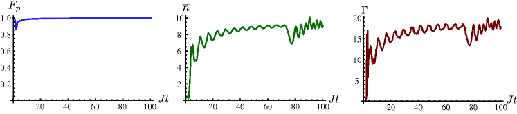
Figure 8: (Color online) (a): Optimized quantum process fidelity between a generalized amplitude damping channel and the dynamical map here under scrutiny. The process fidelity has been maximized with respect to the parameters of the generalized amplitude damping channel at each instant of time. In panel (b) and (c) we show the time-behavior of $\mu$ and $\Gamma$. An analogous behavior is found for $\gamma$. The time-dependence of the last two parameters, and in particular their positivity, are fully in line with the Markovian nature of the qubit effective dynamics.

This gives strong numerical indications that our process is an homogenizing, time-dependent Markovian channel.

III Conclusions

We have studied the dynamics of a qubit interacting via energy-exchange mechanisms with a spin chain under the viewpoint of a recently proposed measure for non-Markovianity breuer09 . We have provided an extensive characterization of the effective open-system evolution experienced by the qubit, often giving fully analytical expressions for the measure of non-Markovianity and an operative recipe for its experimental determination under certain conditions. Our investigation has allowed us to reveal various features of the non-Markovianity measure and to relate them to general properties of the overall $Q-\Gamma$ system. In particular, we have focused on the existence of unexpected points in the parameter space of the model, where the chosen measure of non-Markovianity is exactly null, so that the qubit evolution corresponds to a Markovian dynamical map. By using techniques typical of quantum process tomography, we have been able to shed light onto the reasons behind the forgetful nature of such peculiar working point, showing, in particular, that the zero-measure dynamical map has a single fixed point corresponding to an almost completely mixed qubit state. We have found an excellent agreement between the effective Markovian map and a generalized amplitude damping channel with an additional (independent) dephasing mechanism. The comparison between the two descriptions allows us to determine the behavior of the effective dephasing and damping rates, which are time-dependent yet positive, in agreement with the Markovian nature of the dynamics at hand breuer09 .

The richness of the qubit open-system dynamics is very interesting. We believe that a more extensive exploration of the possibilities offered by the tunability of the degree of Markovianity in such system should be performed so as to understand if a proper and arbitrary “guidance” of the qubit state via the sole manipulation of the properties of the environmental chain is in order. This topic is the focus of our currently ongoing work which will be reported elsewhere futuro .

IV Acknowledgements

FP acknowledges useful discussions with J. Piilo. TJGA thanks Ruggero Vaia for useful discussions and the School of Mathematics and Physics at Queen’s University Belfast for hospitality. CDF is supported by the Irish Research Council for Science, Engineering and Technology. TJGA acknowledges support of the Italian Ministry of Education, University, and Research in the framework of the 2008 PRIN program (Contract No. 2008PARRTS003). MP is supported by EPSRC (EP/G004579/1). MP and FP acknowledge support by the British Council/MIUR British-Italian Partnership Programme 2009-2010.

References

- (1) M. M. Wolf, J. Eisert, T. S. Cubitt, and J. I. Cirac, Phys. Rev. Lett. 101, 150402 (2008).
- (2) A. Rivas, S. F. Huelga, and M. B. Plenio, Phys. Rev. Lett. 105, 050403 (2010).
- (3) H.-P. Breuer, E. M. Laine, and J. Piilo, Phys. Rev. Lett. 103, 210401 (2009); E.-M. Laine, J. Piilo, and H.-P. Breuer, Phys. Rev. A 81, 062115 (2010).
- (4) R.W. Simmonds et al., Phys. Rev. Lett. 93, 077003 (2004); A. Lupascu et al., Phys. Rev. B 80, 172506 (2009); Y. Shalibo et al., Phys. Rev. Lett. 105, 177001 (2010); E. Paladino, L. Faoro, G. Falci, and R. Fazio, ibid. 88, 228304 (2002); A. Shnirman, G. Schön, I. Martin, and Y. Makhlin, ibid. 94, 127002 (2005); G. Falci, A. D’Arrigo, A. Mastellone, and E. Paladino, ibid. 94, 167002 (2005); Y. M. Galperin, B. L. Altshuler, J. Bergli, and D. V. Shantsev, ibid. 96, 097009 (2006); L. Faoro and L. B. Ioffe, ibid. 96, 047001 (2006); E. Paladino, M. Sassetti, G. Falci, and U. Weiss, Phys. Rev. B 77, 041303 (2008); J. Bergli, Y. M. Galperin, B. L. Altshuler, New J. Phys. 11, 025002 (2009); M. Constantin, C. C. Yu, and J. M. Martinis, Phys. Rev. B 79, 094520 (2009).
- (5) X.-M. Lu, X. Wang, and C. P. Sun, Phys. Rev. A 82, 042103 (2010) .
- (6) S. Bose, Contemp. Phys. 48, 13 (2007); S. Bose, Phys. Rev. Lett. 91, 207901 (2003); M. Christandl et al., Phys. Rev. A 71, 032312 (2005); L. Campos Venuti, C. Degli Esposti Boschi, and M. Roncaglia, Phys. Rev. Lett. 99, 060401 (2007); C. Di Franco, M. Paternostro, M. S. Kim, Phys. Rev. Lett. 101, 230502 (2008); F. Plastina and T. J. G. Apollaro, ibid. 99, 177210 (2007); G. Gualdi, V. Kostak, I. Marzoli, and P. Tombesi, Phys. Rev. A 78, 022325 (2008).
- (7) L. Amico, R. Fazio, A. Osterloh, and V. Vedral, Rev. Mod. Phys. 80, 517 (2008).
- (8) Z. Y. Xu, W. L. Yang, and M. Feng, Phys. Rev. A 81, 044105 (2010).
- (9) T. J. G. Apollaro, A. Cuccoli, C. Di Franco, M. Paternostro, F. Plastina, and P. Verrucchi, New J. Phys. 12, 083046 (2010).
- (10) C. Di Franco, M. Paternostro, G. M. Palma, and M. S. Kim, Phys. Rev. A 76, 042316 (2007); C. Di Franco, M. Paternostro, and G. M. Palma, Int. J. Quant. Inf. 6, Supp. 1, 659 (2008).
- (11) A. G. White et al., Phys. Rev. Lett. 83, 3103 (1999); D. James et al., Phys. Rev. A 64, 052312 (2001).
- (12) C. Di Franco, M. Paternostro, and M. S. Kim, Phys. Rev. Lett. 102, 187203 (2009).
- (13) M. A. Nielsen and I. L. Chuang, Quantum Computation and Quantum Information (Cambridge University Press, 2000); I. L. Chuang and M. A. Nielsen, J. Mod. Opt. 44, 2455 (1997).
- (14) W.-C. Yueh, Applied Mathematics E-Notes 5, 66-74 (2005).
- (15) The form of such localized levels has been described by, e.g., L. F. Santos, G. Rigolin, and C. O. Escobar, Phys. Rev. A 69, 042304 (2004); L. F. Santos and G. Rigolin, Phys. Rev. A 71, 032321 (2005); T. J. G. Apollaro and F. Plastina, Phys. Rev. A 74, 062316 (2006).
- (16) P. A. Pury and S. A. Cannas, J. Phys. A 24, L1405-L1414 (1991).
- (17) T. J. Apollaro, A. Cuccoli, A. Fubini, F. Plastina, and P. Verrucchi, Phys. Rev. A 77, 062314 (2008); L. Banchi, T. J. G. Apollaro, A. Cuccoli, R. Vaia, and P. Verrucchi, ibid. 82, 052321 (2010).
- (18) A. Jamiolkowski, Rep. Math. Phys. 3, 275 (1972); M.-D. Choi, Lin. Alg. and Appl. 10, 285 (1975).
- (19) M. B. Ruskai, S. Szarek, and E. Werner, Lin. Alg. Appl. 347, 159-187 (2002).
- (20) W. Son, L. Amico, F. Plastina, and V. Vedral, Phys. Rev. A 79, 022302 (2009).
- (21) T. J. G. Apollaro et al. (work in progress).