Chiral symmetry breaking revisited: the gap equation with lattice ingredients

Abstract

We study chiral symmetry breaking in QCD, using as ingredients in the quark gap equation recent lattice results for the gluon and ghost propagators. The Ansatz employed for the quark-gluon vertex is purely non-Abelian, introducing a crucial dependence on the ghost dressing function and the quark-ghost scattering amplitude. The numerical impact of these quantities is considerable: the need to invoke confinement explicitly is avoided, and the dynamical quark masses generated are of the order of 300 MeV. In addition, the pion decay constant and the quark condensate are computed, and are found to be in good agreement with phenomenology.

One of the major challenges of the strong interactions is to understand the underlying mechanism that generates masses for the quarks and breaks the chiral symmetry (CS). The CS breaking is an inherently nonperturbative phenomena, whose study in the continuum leads almost invariably to a treatment based on the Schwinger-Dyson (SD) equation for the quark propagator (gap equation). As is well known to the SD experts, the existence or not of solutions for this equation depends crucially on the details of its kernel, which is essentially composed by the fully dressed gluon propagator and the quark gluon vertex Aguilar:2010cn . The latter quantity controls the way that ghost sector enters into the gap equation, and introduces a numerically crucial dependence on the ghost dressing function Fischer:2003rp and the quark-ghost scattering amplitude.

In the present talk we report on a recent study of CS breaking Aguilar:2010cn using the SD equation for the quark propagator, supplemented with three nonpertubative ingredients: (i) gluon propagator and (ii) ghost dressing function obtained from large-volume lattice simulations, and (iii) the “one-loop dressed” approximate version of the scalar form factor of the quark-ghost scattering kernel.

The starting point is to express the fully dressed quark propagator in the following general form Roberts:1994dr

$$S^{-1}(p)=/{p}-m-\Sigma(p)=A(p^{2})\,/{p}-B(p^{2})\,,$$ (1)

where $m$ is the bare current quark mass, and $\Sigma(p)$ the quark self-energy. We consider the case without explicit CS breaking, i.e., bare mass m = 0. The dynamical quark mass function can be defined as being the ratio ${\mathcal{M}}(p^{2})=B(p^{2})/A(p^{2})$. Then CS breaking takes place when the scalar component, $B(p^{2})$ develops a non-zero value.

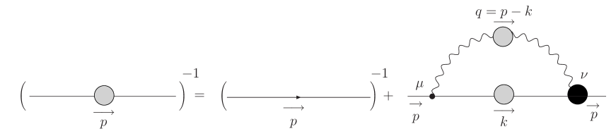
Figure 1: The quark SD equation (gap equation).

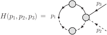
Figure 2: The quark-ghost scattering kernel.

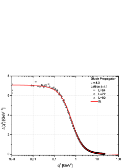
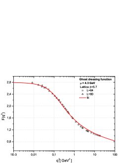
Figure 3: Lattice results for the gluon propagator, $\Delta(q)$, and ghost dressing, $F(q)$ renormalized at $\mu=4.3$ GeV.

The SDE for the quark propagator, which is represented schematically in Fig. 1, can be written as

$$S^{-1}(p)=/{p}-C_{\rm F}g^{2}\int_{k}\gamma_{\mu}S(k)\Gamma_{\nu}(-p,k,q)\Delta^{\mu\nu}(q)\,,$$ (2)

where $q\equiv p-k$, $\int_{k}\equiv\mu^{2\varepsilon}(2\pi)^{-d}\int\!d^{d}k$, with $d=4-\epsilon$ the dimension of space-time. $C_{\rm F}$ is the Casimir eigenvalue in the fundamental representation (for $SU(3)$ $C_{\rm F}=4/3$). The full gluon propagator $\Delta_{\mu\nu}(q)$, in the Landau gauge, has the form

$$\Delta^{\mu\nu}(q)=-i\left[g^{\mu\nu}-\frac{q^{\mu}q^{\nu}}{q^{2}}\right]\Delta(q^{2})\,,$$ (3)

where the non-perturbative behavior of the scalar factor $\Delta(q^{2})$ has been studied in great detail in the continuum Aguilar:2006gr ; Dudal:2008sp and lattice simulations Bogolubsky:2007ud ; Cucchieri:2007md . The fully-dressed quark-gluon vertex $\Gamma_{\nu}(-p,k,q)$ also obeys its own SD equation which unfortunately, it is too complicated. Then, we have to resort to the so called gauge-technique, where a nonperturbative Ansatz for the vertex $\Gamma_{\mu}(p_{1},p_{2},p_{3})$ written in terms of $S(p)$ is constructed, based on the requirement that it should satisfy the fundamental Slavnov-Taylor identity (STI)

$$p_{3}^{\mu}\Gamma_{\mu}=F(p_{3})[S^{-1}(-p_{1})H-{\overline{H}}S^{-1}(p_{2})]\,,$$ (4)

where the ghost dressing function $F(p_{3})$ is related to the full ghost propagator $D(p_{3})$ by $D(p_{3})=iF(p_{3})/p_{3}^{2}$. The quark-ghost scattering kernel $H$, represented in Fig. 2, and its “conjugated” $\overline{H}$ are functions of the momenta $H=H(p_{1},p_{2},p_{3})$, $\overline{H}=\overline{H}(p_{2},p_{1},p_{3})$ respectively.

Both kernels $H$ and ${\overline{H}}$ have the following Lorentz decomposition Davydychev:2000rt

$$H(p_{1},p_{2},p_{3})\!\!\!\!\!\!\!\!\!\! = \!\!\!\!\!\!\!\!\!X_{0}\mathbb{I}+X_{1}/{p_{1}}+X_{2}/{p_{2}}+X_{3}\tilde{\sigma}_{\mu\nu}p_{1}^{\mu}p_{2}^{\nu}\,,$$

$${\overline{H}}(p_{2},p_{1},p_{3})\!\!\!\!\!\!\!\!\! = \!\!\!\!\!\!\!\!\!{\overline{X}}_{0}\mathbb{I}-{\overline{X}}_{2}/{p_{1}}-{\overline{X}}_{1}/{p_{2}}+{\overline{X}}_{3}\tilde{\sigma}_{\mu\nu}p_{1}^{\mu}p_{2}^{\nu},$$ (5)

where the form factors $X_{i}$ are functions of the momenta, $X_{i}=X_{i}(p_{1},p_{2},p_{3})$, and we use the notation ${\overline{X}}_{i}(p_{2},p_{1},p_{3})\equiv X_{i}(p_{1},p_{2},p_{3})$ and $\tilde{\sigma}_{\mu\nu}\equiv\frac{1}{2}[\gamma_{\mu},\gamma_{\nu}]$.

On the other hand, the most general Lorentz structure the longitudinal part of the vertex $\Gamma_{\mu}(p_{1},p_{2},p_{3})$ appearing in the lhs of Eq. (4) is given by  Davydychev:2000rt

$$\Gamma_{\mu}(p_{1},p_{2},p_{3})=L_{1}\gamma_{\mu}+L_{2}(/{p_{1}}-/{p_{2}})(p_{1}-p_{2})_{\mu}$$

$$+L_{3}(p_{1}-p_{2})_{\mu}+L_{4}\tilde{\sigma}_{\mu\nu}(p_{1}-p_{2})^{\nu}\,,$$ (6)

where once again we have suppressed the dependence on the momenta in the form factor $L_{i}$ [i.e. $L_{i}=L_{i}(p_{1},p_{2},p_{3})$].Notice that, the tree level expression is recovered setting $L_{1}=1$ and $L_{2}=L_{3}=L_{4}=0$.

Due to the fact that the behavior of the vertex $\Gamma_{\mu}$ is constrained by the STI of Eq. (4), the form factors $L_{i}$’s appearing into the Eq. (6) will be given in terms of the form factors $X_{i}$’s of Eq. (5).

The full expressions for $L_{i}$’s in terms of the form factors $X_{i}$’s is given in Aguilar:2010cn . For the sake of simplicity, we will show here the case where only the scalar component of the quark-ghost scattering kernel is non-vanishing i.e. $X_{0}\neq 0$ while $X_{i}={\overline{X}}_{i}=0$, for $i\leq 1$. In this limit, we obtain the following expressions

$$L_{1} = F(p_{3})X_{0}(p_{3})\left[\frac{A(p_{1})+A(p_{2})}{2}\right]\,,$$

$$L_{2} = F(p_{3})X_{0}(p_{3})\left[\frac{A(p_{1})-A(p_{2})}{2(p_{1}^{2}-p_{2}^{2})}\right]\,,$$

$$L_{3} = F(p_{3})X_{0}(p_{3})\left[\frac{B(p_{1})-B(p_{2})}{p_{1}^{2}-p_{2}^{2}}\right]\,,$$

$$L_{4} = 0\,.$$ (7)

According the above expression the form factor $L_{i}$’s displays an explicit dependence on the product $F(p_{3})X_{0}(p_{3})$ which contains information about the IR behavior of the ghost propagator. Therefore, the ghost sector couples to the gap equation Eq. (2) through the quark-gluon vertex of Eq. (6). It is interesting to notice that in the limit of $F(p_{3})=X_{0}(p_{3})=1$ the form factors of Eq. (7) reduces to the ones used so-called Ball-Chiu (BC) vertex Ball:1980ay .

We will next insert into Eq. (2) the general quark-gluon vertex of Eq. (6) with the expressions for the form factors $L_{i}$ given in Eq. (7). Defining $p_{1}=-p$, $p_{2}=k$, and $p_{3}=q$ and taking appropriate traces, we derive the expressions for the integral equations satisfied by $A(p^{2})$ and $B(p^{2})$ that schematically can be written as

$$A(p^{2}) = 1+C_{F}g^{2}Z_{c}^{-1}\,\int_{k}\,\frac{{\cal K}_{0}(p-k)}{A^{2}(k^{2})k^{2}+B^{2}(k^{2})}{\cal K}_{A}(k,p)\,,$$

$$B(p^{2}) = C_{F}g^{2}Z_{c}^{-1}\int_{k}\,\frac{{\cal K}_{0}(p-k)}{A^{2}(k^{2})k^{2}+B^{2}(k^{2})}{\cal K}_{B}(k,p)\,,$$ (8)

where the kernel ${\cal K}_{0}(q)$ corresponds to the part that is not altered by the tensorial structure of the quark-gluon vertex, namely ${\cal K}_{0}(q)=\Delta(q)F(q)X_{0}(q)$, while the parts affected are ${\cal K}_{A}(k,p)$ and ${\cal K}_{B}(k,p)$.

The gap equation depends on the nonperturbative form of the three basic Green’s functions, namely $\Delta(q)$, $F(q)$, and $X_{0}(q)$. For $\Delta(q)$ and $F(q)$ we use the recent lattice data obtained by  Bogolubsky:2007ud , and shown in Fig. 3.

We clearly see that both lattice results for $\Delta(q)$ and $F(q)$ are infrared finite. Such a feature can be associated to a purely non-perturbative effect that gives rise to a dynamical gluon mass Cornwall:1982zr , which saturates the gluon propagator in the IR. The appearance of the gluon mass is also responsible for the infrared finiteness of the ghost dressing function, $F(q^{2})$ Aguilar:2006gr ; Boucaud:2008ji , which is shown on the right panel of Fig. 3,

Unfortunately for $X_{0}(q)$ there is no lattice data available, and in order to obtain a non-perturbative estimate for $X_{0}$, we will study “one-loop dressed” scalar contribution of the diagram of Fig. 2 in an approximate kinematic configuration, which simplifies the resulting structures considerably. Specifically, we will assume that $p_{1}=p_{2}\equiv p$, and $p=-q/2$. In doing so, we arrive at (see details in Aguilar:2010cn )

$$X_{0}^{[1]}(q)=1+\frac{1}{4}C_{A}g^{2}q^{2}\int_{k}\left[1-\frac{(k\cdot q)^{2}}{k^{2}q^{2}}\right]\Delta(k)F(k)\frac{F(k+q)}{(k+q)^{4}}\,,$$ (9)

We proceed substituting the fit for the lattice data for $\Delta(q)$ and $F(q)$ presented in Fig. 3 into Eq. (9). The numerical result for $X_{0}^{[1]}(q)$ is shown in the Fig. 4.

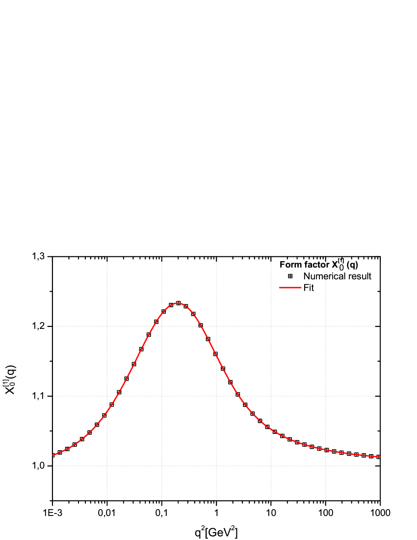
Figure 4: The form factor $X_{0}^{[1]}(q)$ given by Eq. (9.

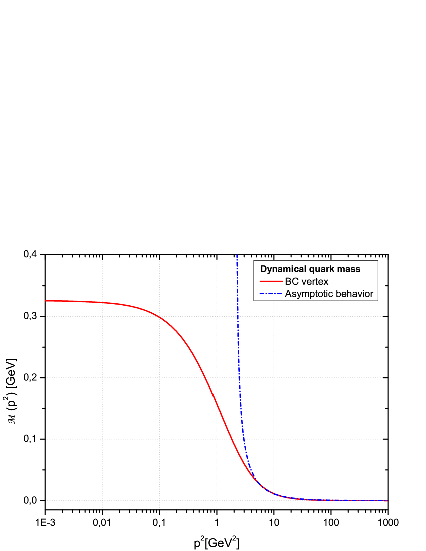
Figure 5: The quark mass ${\mathcal{M}}(p^{2})$ for the BC vertex.

$X_{0}^{[1]}(q)$ shows a maximum located in the intermediate momentum region (around $450$ MeV), while in the UV and IR regions $X_{0}^{[1]}(q)\to 1$. Although this peak is not very pronounced, it is essential for providing to the kernel of the gap equation the enhancement required for the generation of phenomenologically compatible constituent quark masses.

Now we are in position to solve the system formed by Eq.(8) Substituting $\Delta(q^{2})$, $F(q^{2})$, and $X_{0}^{[1]}(q)$ to Eq.(8), with the modification $Z_{c}^{-1}{\cal K}_{A,B}(k,p)\to{\cal K}_{A,B}(k,p)F(p^{2})$, to enforce the correct renormalization group behavior of the dynamical mass (see discussion in Aguilar:2010cn ), we determine numerically the unknown functions $A(p^{2})$ and $B(p^{2})$. The result for the dynamical quark mass ${\mathcal{M}}(p^{2})$ is shown in Fig. 5.

One clearly sees that ${\mathcal{M}}(p^{2})$ freezes out and acquires a finite value in the IR, ${\mathcal{M}}(0)=294$ MeV. In the UV it shows the expected perturbative behavior represented by the blue dashed curve.

With the behavior of the dynamical quark mass at hand, we have computed pion decay constant and the quark condensate and we obtained $f_{\pi}=80.6$ MeV and $\left\langle\bar{q}q\right\rangle(1\,\mbox{GeV}^{2})=\,(217\mbox{MeV})^{3}$ respectively, which are in good agreement with phenomenological results.

References

- (1)
- (2) A. C. Aguilar and J. Papavassiliou, arXiv:1010.5815 [hep-ph].
- (3) C. S. Fischer and R. Alkofer, Phys. Rev. D 67, 094020 (2003).
- (4) C. D. Roberts and A. G. Williams, Prog. Part. Nucl. Phys. 33, 477 (1994).
- (5) A. C. Aguilar and J. Papavassiliou, JHEP 0612, 012 (2006); A. C. Aguilar, D. Binosi and J. Papavassiliou, Phys. Rev. D 78, 025010 (2008); D. Binosi and J. Papavassiliou, Phys. Rept. 479, 1 (2009).
- (6) D. Dudal, J. A. Gracey, S. P. Sorella, N. Vandersickel and H. Verschelde, Phys. Rev. D 78, 065047 (2008).
- (7) I. L. Bogolubsky, E. M. Ilgenfritz, M. Muller-Preussker and A. Sternbeck, PoS LAT2007, 290 (2007).
- (8) A. Cucchieri and T. Mendes, PoS LAT2007, 297 (2007); O. Oliveira and P. J. Silva, PoS QCD-TNT09, 033 (2009).
- (9) A. I. Davydychev, P. Osland and L. Saks, Phys. Rev. D 63, 014022 (2001).
- (10) J. S. Ball and T. W. Chiu, Phys. Rev. D 22, 2542 (1980).
- (11) J. M. Cornwall, Phys. Rev. D 26, 1453 (1982); J. M. Cornwall and J. Papavassiliou, Phys. Rev. D 40, 3474 (1989).
- (12) Ph. Boucaud, J. P. Leroy, A. L. Yaouanc, J. Micheli, O. Pene and J. Rodriguez-Quintero, JHEP 0806 (2008) 012.