Relative information entropy of an inhomogeneous universe

Abstract

In the context of averaging an inhomogeneous cosmological model, we propose a natural measure identical to the Kullback-Leibler relative information entropy, which expresses the distinguishability of the local inhomogeneous density field from its spatial average on arbitrary compact domains. This measure is expected to be an increasing function in time and thus to play a significant role in studying gravitational entropy. To verify this conjecture, we explore the time evolution of the measure using the linear perturbation theory of a spatially flat FLRW model and a spherically symmetric nonlinear solution. We discuss the generality and conditions for the time-increasing nature of the measure, and also the connection to the backreaction effect caused by inhomogeneities.

1 Introduction

Modern cosmology is based on the hypothesis called the Cosmological Principle, and the universe is assumed to be successfully described by a homogeneous and isotropic Friedmann-Lemaître-Robertson-Walker (FLRW) universe model on large scales. In spite of its simplicity, this hypothesis is highly non-trivial because a realistic universe model should include local inhomogeneities, and the physical property of such a realistic model averaged over a sufficiently large scale does not necessarily coincide with that of the FLRW universe. The difference between a spatially averaged inhomogeneous universe and the FLRW universe has been emphasized by Ellis ellis1984 and studied since the pioneering works by Futamase futamase1988 ; futamase1996 . This topic is now widely noticed in the context of dark energy cosmology; the effect of inhomogeneities may be an alternative to introducing an exotic matter for the cosmic acceleration. (See, e.g. Ref. kolb2006 ; Refs. rasanen2006 ; buchert2008 for comprehensive reviews.)

In quantifying how a realistic inhomogeneous universe model departs from the FLRW one, it would be convenient to utilize some measure of inhomogeneity. In Information Theory, if we have two probability distributions, $\{p_{i}\}$ and $\{q_{i}\}$, and would like to quantify the distinguishability of the two distributions, the relevant quantity is known to be the relative information entropy (sometimes called the Kullback-Leibler divergence) ct1991 :

$$\mathcal{S}_{\mathrm{KL}}\{p\parallel q\}:=\sum_{i}p_{i}\ln\frac{p_{i}}{q_{i}}\,,$$ (1)

where $\{p_{i}\}$ and $\{q_{i}\}$ are the actual and presumed probability distributions, respectively. This relative entropy is positive for $q_{i}\neq p_{i}$, and zero if the two distributions $\{p_{i}\}$ and $\{q_{i}\}$ agree. Note that the $\mathcal{S}_{\mathrm{KL}}\{p\parallel q\}$ is not symmetric for $\{p_{i}\}$ and $\{q_{i}\}$. With the help of the concept of the Kullback-Leibler relative information entropy, we proposed in our previous work hbm2004 a natural measure of inhomogeneity in the universe, in the form

$$\mathcal{S}\{\varrho\parallel\langle\varrho\rangle_{\mathcal{D}}\}:=\int_{\mathcal{D}}\varrho\ln\frac{\varrho}{\langle\varrho\rangle_{\mathcal{D}}}\ \mathrm{d}\mu\,,$$ (2)

where $\varrho$ and $\langle\varrho\rangle_{\mathcal{D}}$ are respectively the actual matter distribution and its spatial average, $\mathrm{d}\mu$ is the Riemannian volume element, and the integration is performed on a compact spatial domain $\mathcal{D}$. Here we have adopted the formulation of averaging inhomogeneous universes developed by one of the authors buchert2000 . We also conjectured that the measure (2) is an increasing function of time for sufficiently large times. Intuitively this measure is likely to have the time-increasing nature, but detailed analyses are required to show it. It is actually significant whether this conjecture is correct because the positive conclusion for the conjecture will lead to the validity of our measure being regarded as entropy in a gravitational system. The possibility that our measure is concerned with gravitational entropy has been discussed in Ref. elbu2005 .

In this paper, we explore the time evolution of the measure using specific models of an inhomogeneous universe, and examine on what condition the time-increasing nature of the measure holds. We employ the linear perturbation theory of a spatially flat FLRW universe and a spherically symmetric nonlinear solution as inhomogeneous universe models, and illustrate the temporal behavior of the measure explicitly with the models.

This paper is organized as follows. In the next section, we give a brief review of the formalism of averaging inhomogeneous universes by following Ref. buchert2000 . In the section 3, we introduce a measure of inhomogeneity analogous to the Kullback-Leibler divergence, and derive the time derivatives of the measure with a general consideration for the time-increasing nature of the measure. We present illustrative examples of the time evolution of the measure using the linear perturbation theory and a spherically symmetric exact solution, in the sections 4 and 5, respectively. Finally in the section 6, we summarize our results and give an outlook.

2 Basics of averaging inhomogeneous universes

Let us start by recalling the basic equations that govern the dynamics of a spatially averaged inhomogeneous universe, along the formulation developed by one of the authors buchert2000 ; buchert2001 . We shall restrict our consideration, for simplicity, to an irrotational pressureless fluid with energy density $\varrho$ and four-velocity $u^{\mu}$, and work in a time-orthogonal foliation with the line element

$$\mathrm{d}s^{2}=-\mathrm{d}t^{2}+g_{ij}\mathrm{d}X^{i}\mathrm{d}X^{j}\,,$$ (3)

where $X^{i}$ are coordinates in the $t=\mathrm{const.}$ hypersurfaces (with three-metric $g_{ij}$) that are comoving with the fluid so that the four-velocity $u^{\mu}=(1,\mathbf{0})$. It is convenient for a description of the dynamics to use the expansion tensor $\Theta_{ij}:=(1/2)\dot{g_{ij}}$, where an overdot $(\dot{\ })$ denotes time derivative, and its trace $\theta:=g^{ij}\Theta_{ij}$ (the local expansion rate), and the traceless part $\sigma_{ij}:=\Theta_{ij}-(1/3)\theta g_{ij}$ (the shear tensor). Using these quantities as dynamical variables, the continuity equation and the Raychaudhuri equation are written as

$$\dot{\varrho}+\varrho\theta=0\,,$$ (4)

$$\dot{\theta}=-4\pi G\varrho-\frac{1}{3}\theta^{2}-2\sigma^{2}\,,$$ (5)

where $\sigma^{2}:=(1/2)\sigma^{i}_{\ j}\sigma^{j}_{\ i}$ is the rate of shear squared.

We define averaging of a scalar quantity $A(t,X^{i})$ by the Riemannian volume average over a compact spatial domain $\mathcal{D}$:

$$\langle A(t,X^{i})\rangle_{\mathcal{D}}:=\frac{1}{V_{\mathcal{D}}}\int_{\mathcal{D}}A(t,X^{i})\sqrt{g}\ \mathrm{d}^{3}X\ ;\qquad V_{\mathcal{D}}(t):=\int_{\mathcal{D}}\sqrt{g}\ \mathrm{d}^{3}X\,,$$ (6)

with the Riemannian volume element $\mathrm{d}\mu:=\sqrt{g}\ \mathrm{d}^{3}X$,   $g:=\det(g_{ij})$, of the spatial hypersurfaces of constant time. We also introduce an effective scale factor via the volume (normalized by the volume of the initial domain $V_{{\mathcal{D}}_{\mathrm{i}}}$), $a_{\mathcal{D}}(t):=(V_{\mathcal{D}}(t)/V_{{\mathcal{D}}_{\mathrm{i}}})^{1/3}$. Then the averaged expansion rate is expressed in terms of the effective scale factor as

$$\langle\theta\rangle_{\mathcal{D}}=\frac{\dot{V}_{\mathcal{D}}}{V_{\mathcal{D}}}=3\frac{\dot{a}_{\mathcal{D}}}{a_{\mathcal{D}}}\,.$$ (7)

The key concept in the averaging formalism is non-commutativity of two operations, spatial average and time evolution. This is expressed by a commutation rule for the averaging of a scalar field $A$ buchert2000 ; buchert2001 ; bueh1997 ; rskb1997 :

$$\frac{\partial}{\partial t}\langle A\rangle_{\mathcal{D}}-\left\langle\frac{\partial A}{\partial t}\right\rangle_{\mathcal{D}}=\langle A\theta\rangle_{\mathcal{D}}-\langle A\rangle_{\mathcal{D}}\langle\theta\rangle_{\mathcal{D}}=\langle\delta A\,\delta\theta\rangle_{\mathcal{D}}\,,$$ (8)

where $\delta A:=A-\langle A\rangle_{\mathcal{D}}$ and $\delta\theta:=\theta-\langle\theta\rangle_{\mathcal{D}}$ represent the deviations of local values of the fields from their averages. Averaging Eqs. (4) and (5) with the help of Eq. (8) yields

$$\frac{\partial}{\partial t}\langle\varrho\rangle_{\mathcal{D}}+\langle\varrho\rangle_{\mathcal{D}}\langle\theta\rangle_{\mathcal{D}}=0\,,$$ (9)

$$3\frac{\ddot{a}_{\mathcal{D}}}{a_{\mathcal{D}}}+4\pi G\langle\varrho\rangle_{\mathcal{D}}=Q_{\mathcal{D}}\ ;\qquad Q_{\mathcal{D}}:=\frac{2}{3}\left(\langle\theta^{2}\rangle_{\mathcal{D}}-\langle\theta\rangle_{\mathcal{D}}^{2}\right)-2\langle\sigma^{2}\rangle_{\mathcal{D}}\,,$$ (10)

where $Q_{\mathcal{D}}$ is the ‘kinematical backreaction term’, which appears due to inhomogeneities of cosmic matter distribution and leads the effective cosmic expansion given by $a_{\mathcal{D}}$ to deviate from the Friedmannian one. Equation (10) tells us that the kinematical backreaction term consists of the fluctuation of the expansion rate and the averaged shear rate; the former plays the role of effective negative pressure, and the latter can be regarded as additional matter density.

3 Relative information entropy

In order to introduce a quantity that measures how the universe is inhomogeneous within the formulation explained in the previous section, we pay particular attention to the commutation rule for the matter density field:

$$\frac{\partial}{\partial t}\langle\varrho\rangle_{\mathcal{D}}-\left\langle\frac{\partial\varrho}{\partial t}\right\rangle_{\mathcal{D}}=\langle\varrho\theta\rangle_{\mathcal{D}}-\langle\varrho\rangle_{\mathcal{D}}\langle\theta\rangle_{\mathcal{D}}=\langle\delta\varrho\,\delta\theta\rangle_{\mathcal{D}}\,.$$ (11)

This means that the time evolution of the averaged density field does not coincide with the average of the density field evolved locally. We consider that the difference between $\langle\varrho\rangle_{\mathcal{D}}^{\cdot}$ and $\langle\dot{\varrho}\rangle_{\mathcal{D}}$ leads to the entropy production for the matter density field. This idea brings us to write

$$\frac{\partial}{\partial t}\langle\varrho\rangle_{\mathcal{D}}-\left\langle\frac{\partial\varrho}{\partial t}\right\rangle_{\mathcal{D}}=-\frac{\dot{\mathcal{S}}}{V_{\mathcal{D}}}\,,$$ (12)

where $\mathcal{S}$ is an entropy associated with the density field. Looking for a functional of the matter density field that satisfies Eq. (12), we find that, interestingly, the answer is hbm2004 :

$$\mathcal{S}\{\varrho\parallel\langle\varrho\rangle_{\mathcal{D}}\}:=\int_{\mathcal{D}}\varrho\ln\frac{\varrho}{\langle\varrho\rangle_{\mathcal{D}}}\sqrt{g}\ \mathrm{d}^{3}X\,,$$ (13)

which is analogous to the Kullback-Leibler relative information entropy, Eq. (1). Note that, for strictly positive density, $\varrho>0$, the entropy $\mathcal{S}\{\varrho\parallel\langle\varrho\rangle_{\mathcal{D}}\}$ is positive definite if $\varrho\neq\langle\varrho\rangle_{\mathcal{D}}$, and $\mathcal{S}=0$ if and only if $\varrho=\langle\varrho\rangle_{\mathcal{D}}$.

Let us explore the temporal behavior of the relative information entropy $\mathcal{S}\{\varrho\parallel\langle\varrho\rangle_{\mathcal{D}}\}$ to verify whether the $\mathcal{S}$ possesses the time-increasing nature. From Eqs. (11) and (12), the time derivative of the entropy is immediately found to give

$$\frac{\mathrm{d}}{\mathrm{d}t}\mathcal{S}\{\varrho\parallel\langle\varrho\rangle_{\mathcal{D}}\}=-\int_{\mathcal{D}}\delta\varrho\,\delta\theta\sqrt{g}\ \mathrm{d}^{3}X=-V_{\mathcal{D}}\langle\delta\varrho\,\delta\theta\rangle_{\mathcal{D}}\,.$$ (14)

We expect from Eq. (14) that the time derivative of $\mathcal{S}$ will generally be positive in view of cosmological structure formation, because, on average, an overdense region ($\delta\varrho>0$) tends to contract ($\delta\theta<0$) to form a cluster, and an underdense region ($\delta\varrho<0$) tends to expand ($\delta\theta>0$) to form a void. To be more precise, however, how inhomogeneities evolve depends on initial conditions, particularly at an early stage of the evolution. For example, a fluid element included in an overdense region does not necessarily have an initial expansion rate with the direction of contracting, because the density field and the local expansion rate are given independently in the initial data setting. At a sufficiently late stage, the effect of initial conditions will get weaker and inhomogeneities will evolve according to the intuitive manner as we mentioned above, leading to the positivity of the time derivative of the entropy. It is therefore plausible that, even if the time derivative of the entropy is negative temporarily, it will become positive eventually. This idea implies the importance of examining whether the second time derivative of the entropy is positive, i.e. the time-convexity of the entropy. Differentiation of Eq. (14), together with Eqs. (5) and (8), yields

$$\frac{1}{V_{\mathcal{D}}}\frac{\mathrm{d}^{2}}{\mathrm{d}t^{2}}\mathcal{S}\{\varrho\parallel\langle\varrho\rangle_{\mathcal{D}}\}=4\pi G\left(\Delta\varrho\right)^{2}+\langle\varrho\rangle_{\mathcal{D}}\left(\Delta\theta\right)^{2}+\frac{1}{3}\langle\delta\varrho\,\delta\theta^{2}\rangle_{\mathcal{D}}+2\langle\delta\varrho\,\delta\sigma^{2}\rangle_{\mathcal{D}}\,,$$ (15)

where $\Delta\varrho:=\sqrt{\langle(\delta\varrho)^{2}\rangle_{\mathcal{D}}}$ and $\Delta\theta:=\sqrt{\langle(\delta\theta)^{2}\rangle_{\mathcal{D}}}$ are the fluctuation amplitudes of density and expansion, respectively. Using the formula

$$\delta(\theta^{2})=2\langle\theta\rangle_{\mathcal{D}}\delta\theta+(\delta\theta)^{2}-(\Delta\theta)^{2}\,,$$ (16)

the second time derivative of the entropy, Eq. (15), is rewritten as

$$\frac{\ddot{\mathcal{S}}}{V_{\mathcal{D}}} = 4\pi G\left(\Delta\varrho\right)^{2}+\frac{1}{3}\langle\varrho(\delta\theta)^{2}\rangle_{\mathcal{D}}+\frac{2}{3}\langle\varrho\rangle_{\mathcal{D}}\left(\Delta\theta\right)^{2}+2\langle\delta\varrho\,\delta\sigma^{2}\rangle_{\mathcal{D}}+\frac{2}{3}\langle\theta\rangle_{\mathcal{D}}\langle\delta\varrho\,\delta\theta\rangle_{\mathcal{D}}$$ (17)

$$= 4\pi G\left(\Delta\varrho\right)^{2}+\frac{1}{3}\langle\varrho(\delta\theta)^{2}\rangle_{\mathcal{D}}+2\langle\varrho\sigma^{2}\rangle_{\mathcal{D}}+\langle\varrho\rangle_{\mathcal{D}}Q_{\mathcal{D}}-\frac{2}{3}\langle\theta\rangle_{\mathcal{D}}\frac{\dot{\mathcal{S}}}{V_{\mathcal{D}}}\,.$$ (18)

In order to clarify the conditions under which the positivity of $\dot{\mathcal{S}}$ holds, the sign of the second time derivative $\ddot{\mathcal{S}}$ is crucial, in particular at the instant $t=t_{\mathrm{c}}$ when $\dot{\mathcal{S}}=0$. If $\ddot{\mathcal{S}}(t=t_{\mathrm{c}})$ is shown to be positive, we can conclude that $\dot{\mathcal{S}}$ is always positive thereafter. Note that, from Eq. (18), this applies to the case when the backreaction term $Q_{\mathcal{D}}$ is positive at $t=t_{\mathrm{c}}$. One typical behavior of $\dot{\mathcal{S}}$ will be the following: suppose that $\dot{\mathcal{S}}$ is negative at some time for an averaging domain $\mathcal{D}$ large enough for the averaged expansion rate $\langle\theta\rangle_{\mathcal{D}}>0$ and the averaged shear rate $\langle\sigma^{2}\rangle_{\mathcal{D}}\approx 0$. Then from Eq. (18), $\ddot{\mathcal{S}}$ is positive and thus $\dot{\mathcal{S}}$ increases with time. If $\dot{\mathcal{S}}$ is not bounded by a negative value, $\dot{\mathcal{S}}$ reaches zero at $t=t_{\mathrm{c}}$ and stays positive thereafter.

4 Evolution of the entropy in the linear regime

In what follows, we illustrate the temporal behavior of the entropy $\mathcal{S}$ by using specific models. First let us observe the positivity of $\dot{\mathcal{S}}$ using the linear perturbation theory, which is valid in the early stage of structure formation in the universe, where the deviation from a homogenous and isotropic background is small. This illustrative calculation with the linear perturbation theory is, in a sense, most intuitive and easiest to carry out. The average properties of an inhomogeneous universe constructed with the linear perturbation theory have been investigated in Ref. lischwarz2007 . We follow Ref. lischwarz2007 in the method of the calculation performed in this section.

Suppose that the three-metric is written as $g_{ij}=a(t)^{2}(\gamma_{ij}+h_{ij})$ with the Friedmannian scale factor $a(t)$, the background metric $\gamma_{ij}$, and metric perturbation $h_{ij}$, and a scalar quantity $A(t,X^{i})$ is divided into a homogeneous part $A_{\mathrm{H}}(t)$ and an inhomogeneous perturbation $A_{\mathrm{p}}(t,X^{i})$, which is associated with $h_{ij}$. The spatial average $\langle A\rangle_{\mathcal{D}}$ is then represented in terms of perturbation variables as

$$\langle A\rangle_{\mathcal{D}}:=\frac{1}{V_{\mathcal{D}}}\int_{\mathcal{D}}A\sqrt{g}\ \mathrm{d}^{3}X=A_{\mathrm{H}}+\langle A_{\mathrm{p}}\rangle_{\gamma}+\frac{1}{2}\left(\langle A_{\mathrm{p}}h\rangle_{\gamma}-\langle A_{\mathrm{p}}\rangle_{\gamma}\langle h\rangle_{\gamma}\right)+\mathcal{O}(h^{3})\,,$$ (19)

where $\langle\cdot\rangle_{\gamma}:=\int_{\mathcal{D}}(\cdot)\sqrt{\gamma}\ \mathrm{d}^{3}X/\int_{\mathcal{D}}\sqrt{\gamma}\ \mathrm{d}^{3}X$ ($\gamma:=\det(\gamma_{ij})$) denotes the average defined on the background three-space, and $h:=\gamma^{ij}h_{ij}$. Introducing another scalar quantity $B(t,X^{i})=B_{\mathrm{H}}(t)+B_{\mathrm{p}}(t,X^{i})$ with a homogeneous part $B_{\mathrm{H}}(t)$ and a perturbation $B_{\mathrm{p}}(t,X^{i})$, we have the following useful formula:

$$\langle\delta A\,\delta B\rangle_{\mathcal{D}}=\langle A_{\mathrm{p}}B_{\mathrm{p}}\rangle_{\gamma}-\langle A_{\mathrm{p}}\rangle_{\gamma}\langle B_{\mathrm{p}}\rangle_{\gamma}+\mathcal{O}(h^{3})\,.$$ (20)

The scalar-mode solution for the linear metric perturbation $h_{ij}$ in a spatially flat background without a cosmological constant is lischwarz2007 ; peebles1980

$$h_{ij}=\frac{20}{9}\Psi\gamma_{ij}+2D_{+}(t)\Psi_{|ij}+2D_{-}(t)\Phi_{|ij}\,,$$ (21)

where $\Psi=\Psi(X^{i})$ and $\Phi=\Phi(X^{i})$ are arbitrary functions of only spatial coordinates $X^{i}$, determined by initial conditions,  $|$ denotes covariant derivative with respect to $\gamma_{ij}$, and $D_{+}(t)=t^{2/3}$ and $D_{-}(t)=t^{-1}$ are time-dependent factors of the growing and decaying modes, respectively. The energy density and the expansion rate are then given as

$$\varrho = \varrho_{\mathrm{H}}\left(1-t^{2/3}\nabla^{2}\Psi-t^{-1}\nabla^{2}\Phi\right)\,,$$ (22)

$$\theta = 3\frac{\dot{a}}{a}+\frac{2}{3}t^{-1/3}\nabla^{2}\Psi-t^{-2}\nabla^{2}\Phi\,,$$ (23)

where $\varrho_{\mathrm{H}}=\varrho_{\mathrm{H}}(t)$ is the energy density of the homogeneous background, and $\nabla^{2}(\cdot):=\gamma^{ij}(\cdot)_{|ij}$.

Inserting Eqs. (22) and (23) into Eq. (20), the time derivative of the entropy is calculated straightforwardly as, to the leading order,

$$4\pi G\frac{\dot{\mathcal{S}}}{V_{\mathcal{D}}} = \frac{4}{9}t^{-5/3}\left[\langle(\nabla^{2}\Psi)^{2}\rangle_{\gamma}-\langle\nabla^{2}\Psi\rangle_{\gamma}^{2}\right]-\frac{2}{9}t^{-10/3}\left[\langle\nabla^{2}\Psi\ \nabla^{2}\Phi\rangle_{\gamma}-\langle\nabla^{2}\Psi\rangle_{\gamma}\langle\nabla^{2}\Phi\rangle_{\gamma}\right]$$ (24)

$$-\frac{2}{3}t^{-5}\left[\langle(\nabla^{2}\Phi)^{2}\rangle_{\gamma}-\langle\nabla^{2}\Phi\rangle_{\gamma}^{2}\right]\,.$$

Equation (24) tells us that, if the dynamics of inhomogeneity is dominated by the growing mode, $\dot{\mathcal{S}}$ is positive, meaning that the universe becomes more and more inhomogeneous. At early times, the decaying mode may dominate the growing one, and then $\dot{\mathcal{S}}<0$, which implies that the universe can temporarily become less and less inhomogeneous, but for large enough times, the growing mode is expected to dominate and $\dot{\mathcal{S}}>0$ eventually. One exception is the case where there is no growing mode, but it is quite rare and unphysical, and we can ignore it safely. Thus on the positivity of $\dot{\mathcal{S}}$ in the linear regime, we can claim that the time derivative $\dot{\mathcal{S}}$ becomes positive at least for sufficiently large times, unless the growing mode is exactly zero.

In order to show the above fact from another point of view, let us consider the second time derivative $\ddot{\mathcal{S}}$, Eq. (15). Estimating each term of the right-hand side of Eq. (15) with the linear perturbation theory, we find that the leading order of the last term is $\mathcal{O}(h^{3})$ while that of the other terms is $\mathcal{O}(h^{2})$. Hence the last term can be neglected in this consideration. In addition, we can utilize the following approximate formula in the linear regime:

$$\langle\delta\varrho\,\delta\theta^{2}\rangle_{\mathcal{D}}\approx 2\langle\theta\rangle_{\mathcal{D}}\langle\delta\varrho\,\delta\theta\rangle_{\mathcal{D}}\,,$$ (25)

and thus we obtain

$$\frac{\ddot{\mathcal{S}}}{V_{\mathcal{D}}}\approx 4\pi G\left(\Delta\varrho\right)^{2}+\langle\varrho\rangle_{\mathcal{D}}\left(\Delta\theta\right)^{2}+\frac{2}{3}\langle\theta\rangle_{\mathcal{D}}\langle\delta\varrho\,\delta\theta\rangle_{\mathcal{D}}\,.$$ (26)

We find from Eq. (26) that, when $\dot{\mathcal{S}}<0$, the second derivative $\ddot{\mathcal{S}}$ is positive because all terms in the right-hand side of Eq. (26) are positive; if $\dot{\mathcal{S}}=0$ at an instant $t=t_{\mathrm{c}}$, the second derivative $\ddot{\mathcal{S}}$ at $t=t_{\mathrm{c}}$ is positive. Therefore, $\dot{\mathcal{S}}$ is always going to be positive at $t=t_{\mathrm{c}}$, and thereafter stays positive, as far as the dynamics is in the linear regime.

These facts are also understood directly by an explicit form of the second time derivative, written in terms of the linear perturbations. It is actually given as, to the leading order,

$$4\pi G\frac{\ddot{\mathcal{S}}}{V_{\mathcal{D}}} = \frac{4}{27}t^{-8/3}\left[\langle(\nabla^{2}\Psi)^{2}\rangle_{\gamma}-\langle\nabla^{2}\Psi\rangle_{\gamma}^{2}\right]+\frac{8}{27}t^{-13/3}\left[\langle\nabla^{2}\Psi\ \nabla^{2}\Phi\rangle_{\gamma}-\langle\nabla^{2}\Psi\rangle_{\gamma}\langle\nabla^{2}\Phi\rangle_{\gamma}\right]$$ (28)

$$+2t^{-6}\left[\langle(\nabla^{2}\Phi)^{2}\rangle_{\gamma}-\langle\nabla^{2}\Phi\rangle_{\gamma}^{2}\right]$$

$$= \frac{4}{27}t^{-8/3}\left[\left\langle(\nabla^{2}\Psi+t^{-5/3}\nabla^{2}\Phi)^{2}\right\rangle_{\gamma}-\left\langle\nabla^{2}\Psi+t^{-5/3}\nabla^{2}\Phi\right\rangle_{\gamma}^{2}\right]$$

$$+\frac{50}{27}t^{-6}\left[\langle(\nabla^{2}\Phi)^{2}\rangle_{\gamma}-\langle\nabla^{2}\Phi\rangle_{\gamma}^{2}\right]\quad\geq 0\,.$$

Hence we obtain the following proposition in the linear regime: The second time derivative $\ddot{\mathcal{S}}$ is positive definite in the linear regime. Therefore, even if $\dot{\mathcal{S}}$ is negative for a while, $\dot{\mathcal{S}}$ is always going to be positive. Once $\dot{\mathcal{S}}$ arrives at zero, $\dot{\mathcal{S}}$ is always positive thereafter during the linear regime.

5 Nonlinear example with the LTB model

We proceed in this section to explore the time evolution of the relative information entropy $\mathcal{S}\{\varrho\parallel\langle\varrho\rangle_{\mathcal{D}}\}$ in the nonlinear regime with the spherically symmetric Lemaître–Tolman–Bondi (LTB) solution. This exact solution of Einstein’s equations is often employed as a model of an inhomogeneous universe krasinski1997 ; enqvist2008 ; hellaby2009 ; celerier2010 . The line element of the LTB solution reads

$$\mathrm{d}s^{2}=-\mathrm{d}t^{2}+\frac{r^{\prime 2}}{1+f}\mathrm{d}R^{2}+r^{2}(\mathrm{d}\vartheta^{2}+\sin^{2}\vartheta\mathrm{d}\phi^{2})\,,$$ (29)

where a prime $(\ ^{\prime})$ denotes $\partial/\partial R$, $f=f(R)$ is an arbitrary function of the comoving radial coordinate $R$ with $f>-1$, and $r=r(t,R)$. Then Einstein’s equations yield

$$8\pi G\varrho=\frac{F^{\prime}}{r^{\prime}r^{2}}\,,$$ (30)

$$\dot{r}^{2}=\frac{F(R)}{r}+f(R)\,,$$ (31)

where $F(R)$ is another arbitrary function, which represents the initial mass distribution. The solutions of Eq. (31) can be expressed in the following form:

(i) $f>0$:

$$r=\frac{F}{2f}(\cosh\eta-1)\,,\qquad t-T(R)=\frac{F}{2f^{3/2}}(\sinh\eta-\eta)\,,$$ (32)

(ii) $f<0$:

$$r=\frac{F}{-2f}(1-\cos\eta)\,,\qquad t-T(R)=\frac{F}{2(-f)^{3/2}}(\eta-\sin\eta)\,,$$ (33)

(iii) $f=0$:

$$r=\left(\frac{9F}{4}\right)^{1/3}\left(t-T(R)\right)^{2/3}\,,$$ (34)

where $T(R)$ is a third arbitrary function that comes from integrating Eq. (31). In any of these three cases, the expansion rate and the shear rate squared are given as

$$\theta=\frac{\dot{r}^{\prime}}{r^{\prime}}+2\frac{\dot{r}}{r}=\frac{(r^{2}r^{\prime})^{\cdot}}{r^{2}r^{\prime}}\,,\qquad\sigma^{2}=\frac{1}{3}\left(\frac{\dot{r}^{\prime}}{r^{\prime}}-\frac{\dot{r}}{r}\right)^{2}\,.$$ (35)

If we regard the LTB solution as a spatially flat FLRW universe plus spherical linear perturbations, and make a connection between the functions $f(R)$, $F(R)$, and $T(R)$ in the LTB solution, and the functions $\Psi$ and $\Phi$ that appear in Eq. (21) in the linear perturbation theory, we obtain mnk1998 :

$$f=\frac{20}{9}\Psi^{\prime}R\,,\qquad F=\frac{4}{9}R^{3}\left(1+\frac{10}{3}\Psi\right)\,,\qquad T=-\frac{3}{2}\Phi^{\prime}R^{-1}\,.$$ (36)

These relations tell us that the functions $f(R)$ and $T(R)$ correspond to the growing and decaying modes in the linear perturbation theory, respectively.

Let us write averaged dynamical variables in the LTB solution. Taking a spherical compact domain ${\mathcal{D}}$:

$${\mathcal{D}}=\left\{(R,\,\vartheta,\,\phi)|\ 0\leq R\leq R_{\mathrm{d}},\ 0\leq\vartheta\leq\pi,\ 0\leq\phi\leq 2\pi\right\}\,,$$

with the comoving radius of the spherical domain $R_{\mathrm{d}}$, we have

$$8\pi G\langle\varrho\rangle_{\mathcal{D}}=\left\langle\frac{F^{\prime}}{r^{2}r^{\prime}}\right\rangle_{\mathcal{D}}=\frac{4\pi}{V_{\mathcal{D}}}\int_{0}^{R_{\mathrm{d}}}\frac{F^{\prime}}{(1+f)^{1/2}}\ \mathrm{d}R\,,$$ (37)

$$\langle\theta\rangle_{\mathcal{D}}=\left\langle\frac{\dot{r}^{\prime}}{r^{\prime}}+2\frac{\dot{r}}{r}\right\rangle_{\mathcal{D}}=\frac{4\pi}{V_{\mathcal{D}}}\int_{0}^{R_{\mathrm{d}}}\frac{(r^{2}r^{\prime})^{\cdot}}{(1+f)^{1/2}}\ \mathrm{d}R\,,$$ (38)

with the volume of the domain $\mathcal{D}$,

$$V_{\mathcal{D}}=4\pi\int_{0}^{R_{\mathrm{d}}}\frac{r^{2}r^{\prime}}{(1+f)^{1/2}}\ \mathrm{d}R\,.$$ (39)

Using Eqs. (30), (35), (37), and (38), the backreaction term $Q_{\mathcal{D}}$ and the time derivative of the entropy in the spherical case become

$$Q_{\mathcal{D}}=\left\langle 2\frac{\dot{r}}{r}\left(2\frac{\dot{r}^{\prime}}{r^{\prime}}+\frac{\dot{r}}{r}\right)\right\rangle_{\mathcal{D}}-\left\langle\frac{\dot{r}^{\prime}}{r^{\prime}}+2\frac{\dot{r}}{r}\right\rangle_{\mathcal{D}}^{2}\,,$$ (40)

$$8\pi G\dot{\mathcal{S}}=\frac{4\pi\dot{V}_{\mathcal{D}}}{V_{\mathcal{D}}}\int_{0}^{R_{\mathrm{d}}}\frac{F^{\prime}\ \mathrm{d}R}{(1+f)^{1/2}}-4\pi\int_{0}^{R_{\mathrm{d}}}\frac{F^{\prime}(r^{2}r^{\prime})^{\cdot}\ \mathrm{d}R}{r^{2}r^{\prime}(1+f)^{1/2}}\,.$$ (41)

In order to illustrate the time evolution of the entropy, we choose the three arbitrary functions, as is suggested in Ref. mathum2001 , as

$$T(R)=0\quad\mbox{for all }\ R\geq 0\,,\qquad f(R)=\left\{\begin{array}[]{cl}-\left(\frac{R}{R_{0}}\right)^{2}\left(1-\frac{R}{R_{0}}\right)^{2}&\quad\mbox{for }\ 0\leq R\leq R_{0}\,,\\ 0&\quad\mbox{for }\ R>R_{0}\,,\end{array}\right.$$ (42)

$$F(R)=\left\{\begin{array}[]{ll}\frac{4}{9}R^{3}&\quad\mbox{for }\ 0\leq R<R_{1}\,,\\ \frac{4}{9}R_{1}^{3}&\quad\mbox{for }\ R_{1}\leq R\leq R_{0}\,,\\ \frac{4}{9}R^{3}\left(\frac{R_{1}}{R_{0}}\right)^{3}&\quad\mbox{for }\ R>R_{0}\,,\end{array}\right.$$ (43)

where $R_{0}$ and $R_{1}$ are constants that satisfy $R_{1}>R_{0}/2$. The inner region ($0\leq R\leq R_{1}$) of this model is the collapsing LTB solution, which is surrounded by a vacuum region ($R_{1}<R\leq R_{0}$), and the outermost region ($R>R_{0}$) is the Einstein-de Sitter universe, i.e. a spatially flat FLRW universe without a cosmological constant. Setting $T(R)=0$ is appropriate for our purpose, because the function $T(R)$ corresponds to the decaying mode in the linear perturbation theory, and its effect disappears for sufficiently large times.

In our illustration, we choose the constants $R_{0}$ and $R_{1}$ so that $R_{1}=3R_{0}/4$, and consider two cases of the radius $R_{\mathrm{d}}$ of the averaging domain: (i) $R_{\mathrm{d}}=R_{0}$, which is called ‘the large domain’, and (ii) $R_{\mathrm{d}}=R_{0}/8$, ‘the small domain’. Note that, in the case of the large domain, the averaging domain contains the collapsing LTB region and the vacuum region, while the small domain consists of only the collapsing LTB region. As the result of the choice of the domain, the evolution of the effective scale factor for the large (small) domain is similar to that of a spatially flat (closed) FLRW universe, as we see in Fig 1.

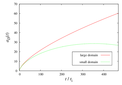
Figure 1: The effective scale factors for the spherical domains are plotted as functions of time. The solid line is for the large domain, and the dashed one for the small domain.

We also present the time evolution of the kinematical backreaction term divided by its initial value for the large and small domains in Fig. 2. In both cases, the backreaction term has, in fact, negative values through the evolution, and thus we find that the results shown in Fig. 2 are consistent with those given in Fig 1.

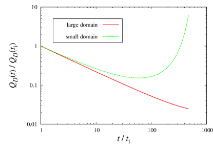
Figure 2: The time evolution of the backreaction term divided by its initial value is plotted. The solid line is for the large domain, and the dashed one for the small domain.

Next we show the time evolution of the time derivative of the entropy, $\dot{\mathcal{S}}(t)$, in Figs. 3 (for the large domain) and 4 (for the small domain). It should be emphasized that $\dot{\mathcal{S}}$ is positive in both cases throughout the evolution in our investigation. In the case of the large domain, however, the $\dot{\mathcal{S}}$ decreases with time temporarily, meaning that the second time derivative $\ddot{\mathcal{S}}$ is negative at early times. We presume that this result is caused by the vacuum region contained in the large domain, because the vacuum is a completely nonlinear structure where the linear perturbation theory does not apply, while the behavior of nonlinear clumps is somewhat similar to that of the linear perturbation at the early stage of the evolution. Detailed investigation is needed on this point.

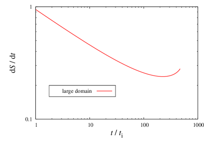
Figure 3: The time derivative of the entropy for the large domain is plotted as a function of time.

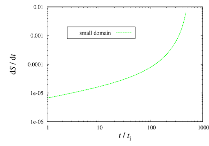
Figure 4: The same as Fig. 3, but for the small domain.

6 Summary and Outlook

In this paper, we study the time evolution of the Kullback-Leibler relative information entropy for cosmic matter distribution which was proposed as a measure of cosmic inhomogeneity in our previous work hbm2004 . Intuitively this entropy is likely to possess the time-increasing nature, but it generally depends on initial conditions. We employ the linear perturbation of a spatially flat FLRW universe and the LTB model to demonstrate that the relative information entropy is convex and increases in time.

We obtain explicit forms of the time derivative and the second time derivative of the entropy through the linear perturbation calculation. They tell us that in the linear regime of cosmic structure formation, the entropy is shown to be an increasing function of time at least for sufficiently late times, even if the entropy decreases temporarily at early times. We also give an illustrative example of the time evolution of the entropy with a nonlinear LTB solution. This illustration also supports the time-increasing nature of the entropy although it shows that the entropy is not always time-convex. It seems from the example whether or not the measure is time-convex depends on the fraction of devoid regions within the averaging domain, i.e. on whether the universe is void-dominated. This will be further investigated in detail in a forthcoming publication.

References

• (1) G. F. R. Ellis, “Relativistic cosmology – Its nature, aims and problems,” in General Relativity and Gravitation, edited by B. Bertotti et al., D. Reidel Publishing Co., Dordrecht, 1984, pp. 215–288.
• (2) T. Futamase, Phys. Rev. Letters 61, 2175–2178 (1988).
• (3) T. Futamase, Phys. Rev. D 53, 681–689 (1996).
• (4) E. W. Kolb, S. Matarrese, and A. Riotto, New J. Phys. 8, 322 (2006), arXiv:astro-ph/0506534.
• (5) S. Räsänen, J. Cosmol. Astropart. Phys. 11 (2006) 003, arXiv:astro-ph/0607626.
• (6) T. Buchert, Gen. Relativ. Gravit. 40, 467–527 (2008), arXiv:0707.2153.
• (7) T. M. Cover and J. A. Thomas, Elements of Information Theory, Wiley-Interscience, New York, 1991.
• (8) A. Hosoya, T. Buchert, and M. Morita, Phys. Rev. Letters 92, 141302-1–4 (2004), arXiv:gr-qc/0402076.
• (9) T. Buchert, Gen. Relativ. Gravit. 32, 105–125 (2000), arXiv:gr-qc/9906015.
• (10) G. F. R. Ellis and T. Buchert, Phys. Letters A 347, 38–46 (2005), arXiv:gr-qc/0506106.
• (11) T. Buchert, Gen. Relativ. Gravit. 33, 1381–1405 (2001), arXiv:gr-qc/0102049.
• (12) T. Buchert and J. Ehlers, Astron. Astrophys. 320, 1–7 (1997), arXiv:astro-ph/9510056.
• (13) H. Russ, M. H. Soffel, M. Kasai, and G. Börner, Phys. Rev. D 56, 2044–2050 (1997), arXiv:astro-ph/9612218.
• (14) N. Li and D. J. Schwarz, Phys. Rev. D 76, 083011-1–15 (2007), arXiv:gr-qc/0702043.
• (15) P. J. E. Peebles, The Large-Scale Structure of the Universe, Princeton University Press, Princeton, NJ, 1980.
• (16) A. Krasiński, Inhomogeneous Cosmological Models, Cambridge University Press, Cambridge, UK, 1997, pp. 100–141.
• (17) K. Enqvist, Gen. Relativ. Gravit. 40, 451–466 (2008), arXiv:0709.2044.
• (18) C. Hellaby, “Modelling Inhomogeneity in the Universe,” in Fifth International School on Field Theory and Gravitation, Proceedings of Science PoS(ISFTG)005, SISSA, Trieste, 2009, arXiv:0910.0350.
• (19) M.-N. Célérier, AIP Conf. Proc. 1241, 767–775 (2010), arXiv:0911.2597.
• (20) M. Morita, K. Nakamura, and M. Kasai, Phys. Rev. D 57, 6094–6103 (1998); Erratum 58, 089903-1 (1998), arXiv:astro-ph/9711026.
• (21) D. R. Matravers and N. P. Humphreys, Gen. Relativ. Gravit. 33, 531–552 (2001), arXiv:gr-qc/0009057.