Electric field induced inversion of the sign of half-integer disclinations in 2D nematic liquid crystals

Abstract

We study the effect of the rotation of an external electric field on the dynamics of half-integer disclination networks in two dimensional nematic liquid crystals with a negative dielectric anisotropy using LICRA, a LIquid CRystal Algorithm developed by the authors. We show that a rotation of $\pi$ of the electric field around an axis of the liquid crystal plane continuously transforms all half-integer disclinations of the network into disclinations of opposite sign via twist disclinations. We also determine the evolution of the characteristic length scale, thus quantifying the impact of the external electric field on the coarsening of the defect network.

I INTRODUCTION

Topological defects play a fundamental role in condensed matter physics de Gennes and Prost (1995); Kleman and Lavrentovich (2003) and cosmology Vilenkin and Shellard (1994). Liquid crystals are an example of a very rich environment where the dynamics of topological defects can be realized experimentally at relatively low costs, making them ideal laboratories for testing different scenarios for defect formation and evolution Chuang et al. (1991, 1993); Zapotocky et al. (1995); Digal et al. (1999); Denniston et al. (2001); Dutta and Roy (2005); de Lózar et al. (2005); Mukai et al. (2007); Bhattacharjee et al. (2008). External fields, such as electric and magnetic fields, can have a significant impact on the orientational order of liquid crystals Kitzerow (1991); Dierking et al. (2005); Alexander and Marenduzzo (2008); Fukuda et al. (2009); Fukuda (2010); de Oliveira et al. (2010) thus affecting the coarsening dynamics of disclination networks. Recently it was shown that the orientation of the applied electric field and the sign of the LC dielectric anisotropy may be used to control the type and topological charge of disclination networks de Oliveira et al. (2010). In Fukuda (2010) a continuous transformation of some $-1/2$ wedge disclination lines into $1/2$ ones was numerically simulated on a cholesteric blue phase of a chiral liquid crystal, through the application of a constant electric field oblique to the line wedge. This provided a numerical realization of a continuous transformation between half-integer disclinations with topological charge of opposite sign Kleman and Lavrentovich (2003).

In the present work we provide a numerical realization of the inversion of the sign of all half-integer disclinations on a 2D nematic LC with a negative dielectric constant induced by the rotation of an external electric field. In our implementation all half-integer disclinations of the network transform into disclinations of opposite sign via twist disclinations. We also consider other dynamical effects associated with the application of the extern electric field on the nematic, by comparing the coarsening of the network under the rotation of the electric field with its evolution under a transformation of the director profile implemented by hand.

The paper is organized as follows. In Sec. II, the equations describing the relaxational dynamics of nematic LC, in terms of a symmetric, traceless order parameter $Q_{\alpha\beta}$, are presented. The numerical techniques are discussed in Sec. III. In Sec. IV the effect of the rotation of an external electric field on the evolution of half-integer disclination networks on a two-dimensional nematic LC with a negative dielectric anisotropy is studied in detail. The conclusions and final remarks are presented in Sec. V

II THE MODEL

The orientational order of a nematic LC without intrinsic biaxiality is described by a symmetric traceless tensor, $Q_{\alpha\beta}$, at every point in space, whose components are given by de Gennes and Prost (1995)

$$Q_{\alpha\beta}=\frac{3}{2}S(n_{\alpha}n_{\beta}-\frac{1}{3}\delta_{\alpha\beta})+\frac{1}{2}T\left(l_{\alpha}l_{\beta}-m_{\alpha}m_{\beta}\right)\,,$$ (1)

where the unit vector ${\bf n}$ is the director, determining the local average orientation of the molecules, ${\bf l}$ is the codirector, associated with the direction of orientational order perpendicular to ${\bf n}$ and ${\bf m}={\bf n}\times{\bf l}$. The variables $S$ and $T$ represent the strength of uniaxial and biaxial ordering, respectively. The values of $S$ and $T$ may be found by the diagonalization of the matrix

$$Q_{\alpha\beta}=\left(\begin{array}[]{ccc}-(S+T)/2&0&0\\ 0&-(S-T)/2&0\\ 0&0&S\end{array}\right)\,,$$ (2)

in a coordinate system where ${\bf n}=(0,0,1)$, ${\bf l}=(0,1,0)$ and ${\bf m}=(1,0,0)$.

Static equilibrium can only be reached for a minimum value of the free energy ($\delta F/\delta Q_{\alpha\beta}=0$). However, the evolution of the order parameter $Q_{\alpha\beta}$ from a given set of initial conditions is not fully specified by the free energy functionals, and further assumptions have to be made on how the minimization process will take place. In the absence of thermal fluctuations and hydrodynamic flow, the time evolution of the order parameter is given by de Gennes (1971)

$${\dot{Q}}_{\alpha\beta}({\bf r},t)=-\Gamma_{\alpha\beta\mu\nu}\frac{\delta F}{\delta Q_{\mu\nu}}\,.$$ (3)

Here the dot represents derivative with respect to the physical time, $t$, and the tensor

$$\Gamma_{\alpha\beta\mu\nu}=\Gamma\left(\delta_{\alpha\mu}\delta_{\beta\nu}+\delta_{\alpha\nu}\delta_{\beta\mu}-\frac{2}{3}\delta_{\alpha\beta}\delta_{\mu\nu}\right)\,,$$ (4)

satisfies $\Gamma_{\alpha\beta\mu\nu}=\Gamma_{\beta\alpha\mu\nu}=\Gamma_{\mu\nu\alpha\beta}$ and $\Gamma_{\alpha\alpha\mu\nu}=0$ thus ensuring that the order parameter $Q_{\alpha\beta}$ remains symmetric and traceless. In the following we shall assume that the kinetic coefficient, $\Gamma$, is a constant.

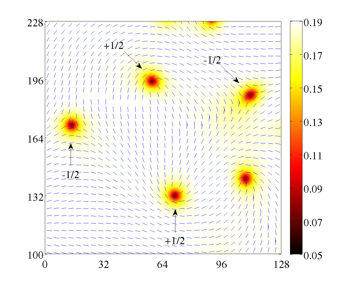
Figure 1: (Color online) Projection of the director ${\bf n}$ onto the two dimensional grid along with the value of the parameter $S$ at every grid point, at $t=499$. Only half-integer disclinations remain due to application of an external electric field along the $z$ direction.

The free energy can be written as

$$F=\int d^{3}{\bf r}\left(\mathcal{F}_{b}+\mathcal{F}_{el}+\mathcal{F}_{E}\right)\,.$$ (5)

The first term, $\mathcal{F}_{b}$, is the bulk free energy density. It describes the nematic-isotropic phase transition and it may be obtained form a local expansion in rotationally invariant powers of the order parameter

$$\mathcal{F}_{b}=\frac{A}{2}\,{\rm Tr}Q^{2}+\frac{B}{3}\,{\rm Tr}Q^{3}+\frac{C}{4}\,({\rm Tr}Q^{2})^{2}\,.$$ (6)

The second term, $\mathcal{F}_{el}$, is the elastic free energy density. Using the one elastic constant approximation the elastic free energy density is given by

$$\mathcal{F}_{el}=\frac{R}{2}\,\partial_{\alpha}Q_{\beta\gamma}\,\partial_{\alpha}Q_{\beta\gamma}\,,$$ (7)

where the constant $R$ is the single elastic constant. The last term in the free energy functional, $\mathcal{F}_{E}$, is the contribution of the effect of an external electric field ${\bf E}$,

$$\mathcal{F}_{E}=-\frac{\tau_{E}}{2}Q_{\alpha\beta}E_{\alpha}E_{\beta}\,,$$ (8)

where $\tau_{E}=2\Delta\epsilon$ and $\Delta\epsilon$ is the dielectric anisotropy. The molecules of a LC with positive dielectric constant, $\Delta\epsilon>0$, tend to orient parallel to the external electric field, ${\bf E}$. On the other hand, if the LC has a negative dielectric constant, $\Delta\epsilon<0$, then the molecules tend to be align perpendicularly to ${\bf E}$.

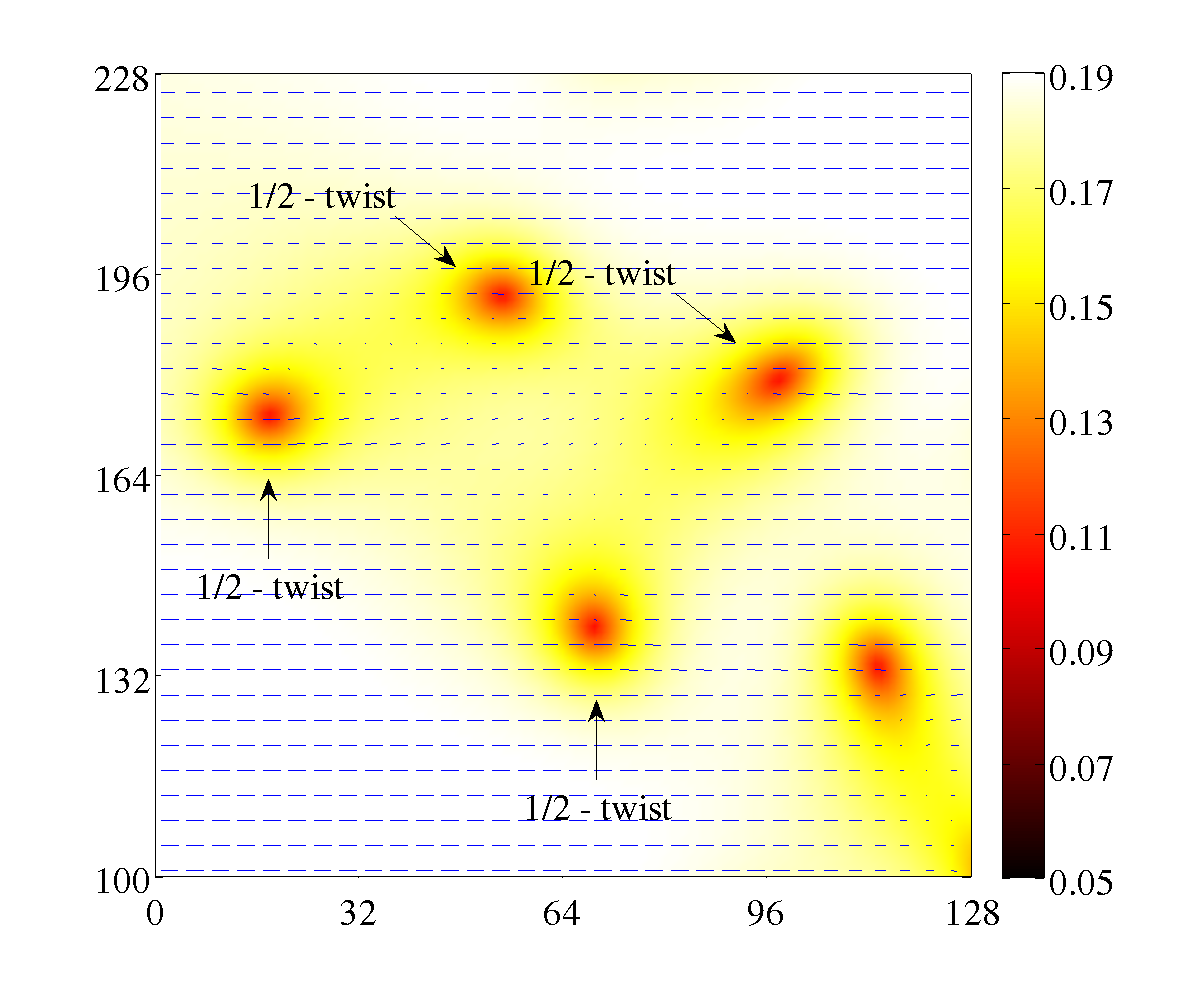
Figure 2: (Color online) Projection of the director ${\bf n}$ onto the two dimensional grid along with the value of the parameter $S$ at every grid point for a single snapshot of simulation $B$ at $t=650$, after the rotation of the electric field by an angle of $\pi/2$. Only half-integer twist disclinations appear in this snapshot.

With this free energy the equation of motion can be written more explicitly as

$${\dot{Q}}_{\alpha\beta}= -\Gamma\left[\right.(A+C\,{\rm Tr}Q^{2})Q_{\alpha\beta}+B\,\mbox{$\hskip 1.00006pt\stackrel{{\scriptstyle\rule{0.4pt}{0.8288pt}\hskip 2.79996pt\!\!\!\overline{\hskip 0.41998pt\vphantom{\rule{0.4pt}{0.0pt}}\hphantom{\mbox{$\displaystyle Q_{\alpha\gamma}Q_{\gamma\beta}$}}\hskip 0.41998pt}\!\!\!\hskip 2.79996pt\rule{0.4pt}{0.8288pt}}}{{Q_{\alpha\gamma}Q_{\gamma\beta}}}\hskip 1.99997pt$ }$$ (9)

$$-R\,Q_{\alpha\beta,\gamma\gamma}-\tau_{E}\mbox{$\hskip 1.00006pt\stackrel{{\scriptstyle\rule{0.4pt}{0.8288pt}\hskip 2.79996pt\!\!\!\overline{\hskip 0.41998pt\vphantom{\rule{0.4pt}{0.0pt}}\hphantom{\mbox{$\displaystyle E_{\alpha}E_{\beta}$}}\hskip 0.41998pt}\!\!\!\hskip 2.79996pt\rule{0.4pt}{0.8288pt}}}{{E_{\alpha}E_{\beta}}}\hskip 1.99997pt$ }\left.\right]\,,$$

where a comma denotes a partial derivative and $\hskip 1.00006pt\stackrel{{\scriptstyle\rule{0.4pt}{0.8288pt}\hskip 2.79996pt\!\!\!\overline{\hskip 0.41998pt\vphantom{\rule{0.4pt}{0.0pt}}\hphantom{\mbox{$\displaystyle X_{\alpha\beta}$}}\hskip 0.41998pt}\!\!\!\hskip 2.79996pt\rule{0.4pt}{0.8288pt}}}{{X_{\alpha\beta}}}\hskip 1.99997pt$ setting an arbitrary real matrix, $X_{\alpha\beta}$, to be a symmetric traceless matrix by the following procedure

$$\mbox{$\hskip 1.00006pt\stackrel{{\scriptstyle\rule{0.4pt}{0.8288pt}\hskip 2.79996pt\!\!\!\overline{\hskip 0.41998pt\vphantom{\rule{0.4pt}{0.0pt}}\hphantom{\mbox{$\displaystyle X_{\alpha\beta}$}}\hskip 0.41998pt}\!\!\!\hskip 2.79996pt\rule{0.4pt}{0.8288pt}}}{{X_{\alpha\beta}}}\hskip 1.99997pt$ }=\frac{1}{2}(X_{\alpha\beta}+X_{\beta\alpha})-\frac{1}{3}\delta_{\alpha\beta}X_{\gamma\gamma}\,.$$ (10)

III NUMERICAL IMPLEMENTATION

All the numerical simulations were performed with LICRA (LIquid CRystal Algorithm), a publicly available set of C codes and MATLAB/OCTAVE routines used to solve Eq. (9) using a standard second-order finite difference algorithm for the spatial derivatives and a second order Runge-Kutta method for the time integration. This software is free and it is available at http://faraday.fc.up.pt/licra de Oliveira et al. (2010).

The order parameter ${\bf Q}$ has 5 degrees of freedom associated with $S$, $T$, $\bf n$ and $\bf l$ ($\bf n$ accounts for two degrees of freedom). The initial conditions for $S$ and $T$ are randomly generated, at every grid point, from uniform distributions in the intervals $[0,2/3]$ and $[0,3S]$, respectively. The director, ${\bf n}$, is also randomly generated, at every grid point, using the spherical vector distribuitions routines in the GNU Scientific Library (GSL) and the codirector, $\bf l$ , was calculated by randomly choosing a direction perpendicular to ${\bf n}$. The eigenvalues and eigenvectors in LICRA are computed using the library GSL.

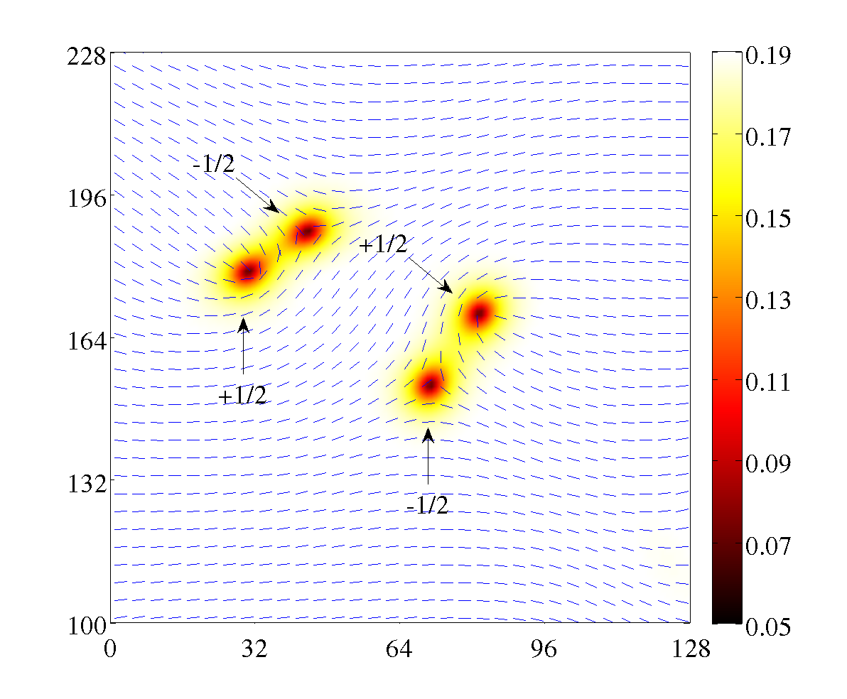
Figure 3: (Color online) Similar to Figs. 2 and 1 but now at $t=900$, ($t>t_{\rm off}$). The sign of all topological charges were inverted with respect to Fig. 1.

In order to determine the evolution of the characteristic scale of the network LICRA numerically calculates the correlation function in Fourier space

$$P({\bf k},t)=\frac{Q_{\alpha\beta}({\bf k},t)Q_{\beta\alpha}({\bf-k},t)}{\int{d^{3}{\bf k}\;Q_{\alpha\beta}({\bf k},t)Q_{\beta\alpha}({\bf-k},t)}}\,,$$ (11)

after setting the infinite wavelength mode $Q_{\alpha\beta}({\bf 0})$ to zero. Here $Q_{\alpha\beta}({\bf k})$ is the Fourier transform of $Q_{\alpha\beta}({\bf r})$ (${\bf k}$ is the wavenumber) and was calculated by using the library Fastest Fourier Transform in the West. The characteristic scale, $L$, can then be defined as

$$\frac{1}{L^{2}}=\langle k^{2}\rangle=\sum_{{\bf k}}k^{2}P({\bf k},t)/\sum_{{\bf k}}P({\bf k},t)\,.$$ (12)

In this paper we have used LICRA to perform high resolution numerical simulations of the dynamics of a texture network in a uniaxial nematic two-dimensional LC under an external electric field. All simulations were performed on a $2048^{2}$ grid (in the $xy$ plane) with parameters $\Delta x=\Delta y=1$, $\Delta t=0.1$, $A=-0.1$, $B=-0.5$, $C=2.67$, $R=1.0$, $\Gamma=1.0$, $|{\bf E}|=0.2/{\sqrt{|\Delta\epsilon|}}$ and $\Delta\epsilon=-0.04$.

IV RESULTS

The evolution of $Q_{\alpha\beta}$ starts with the external electric field switched off. An electric field perpendicular to the plane of the simulation (along the $z$ direction) is connected at $t=300$ and disconnected at $t=350$. This procedure ensures that only half-integer disclinations remain in the simulation de Oliveira et al. (2010). After that, three different simulations have been performed: simulation $A$ with no external electric field, simulation $B$ where a rotating external electric field has been applied between $t_{\rm on}=500$ and $t_{\rm off}=800$ and simulation $C$ where a modification by hand of the director and co-director profiles was made at $t=500$. Fig. 1 shows the value of the order parameter $S$ and the projection of the director ${\bf n}$ onto the two dimensional grid for $t=499$, which is equivalent for simulation $A$, $B$ and $C$.

Figure 4: (Color online) Projection of the director ${\bf n}$ onto the two dimensional grid along with the value of the parameter $S$ at every grid point of a single snapshot of simulation $C$ at $t=900$, after changing the director configuration profile by hand according to Eq. (16). The sign of all topological charges were inverted with respect to Fig. 1.

In simulation $B$ the components of the electric field are given by

$$E_{x} = 0\,,$$

$$E_{y} = |{\bf E}|\sin(\varphi)\,,$$

$$E_{z} = |{\bf E}|\cos(\varphi)\,,$$ (13)

with

$$\varphi=\frac{\pi}{300}\left(t-500\right)\,.$$ (14)

The electric field was applied at $t_{\rm on}=500$ along the $z$ direction and then rotates around the $x$ direction by an angle of $\varphi$, on the $yz$ plane. At each time step ($\Delta t=0.1$) the angle, $\varphi$, was increased by $\pi/3000$ radians until a total angle of $\pi$ (at $t_{\rm off}=800$). The negative dielectric anisotropy, $\Delta\epsilon<0$, ensures that the director remains perpendicular to the field ensuring that ${\bf n}\cdot{\bf E}=0$. If the defect centers were static then, at each time-step, the components of the director would be equal to

$$n_{x} = n_{x_{0}}\,,$$

$$n_{y} = n_{y_{0}}\cos(\varphi)\,,$$

$$n_{z} = -n_{y_{0}}\sin(\varphi)\,,$$ (15)

where $(n_{x_{0}},n_{y_{0}},0)$ are the components of the director at $t=500$ in simulation $A$. In practice this result must be complemented with the coarsening dynamics of the network.

Fig. 2 presents the order parameter $S$ and the projection of the director, ${\bf n}$, onto the two dimensional grid for a snapshot taken from simulation $B$, at $t=650$, when $\varphi=\pi/2$. In this case, the director is given by ${\bf n}=(n_{x_{0}},0,-n_{y_{0}})$ and twist disclinations are formed on the $xz$ plane. Note that the presence of the electric field increases the size of the defect cores.

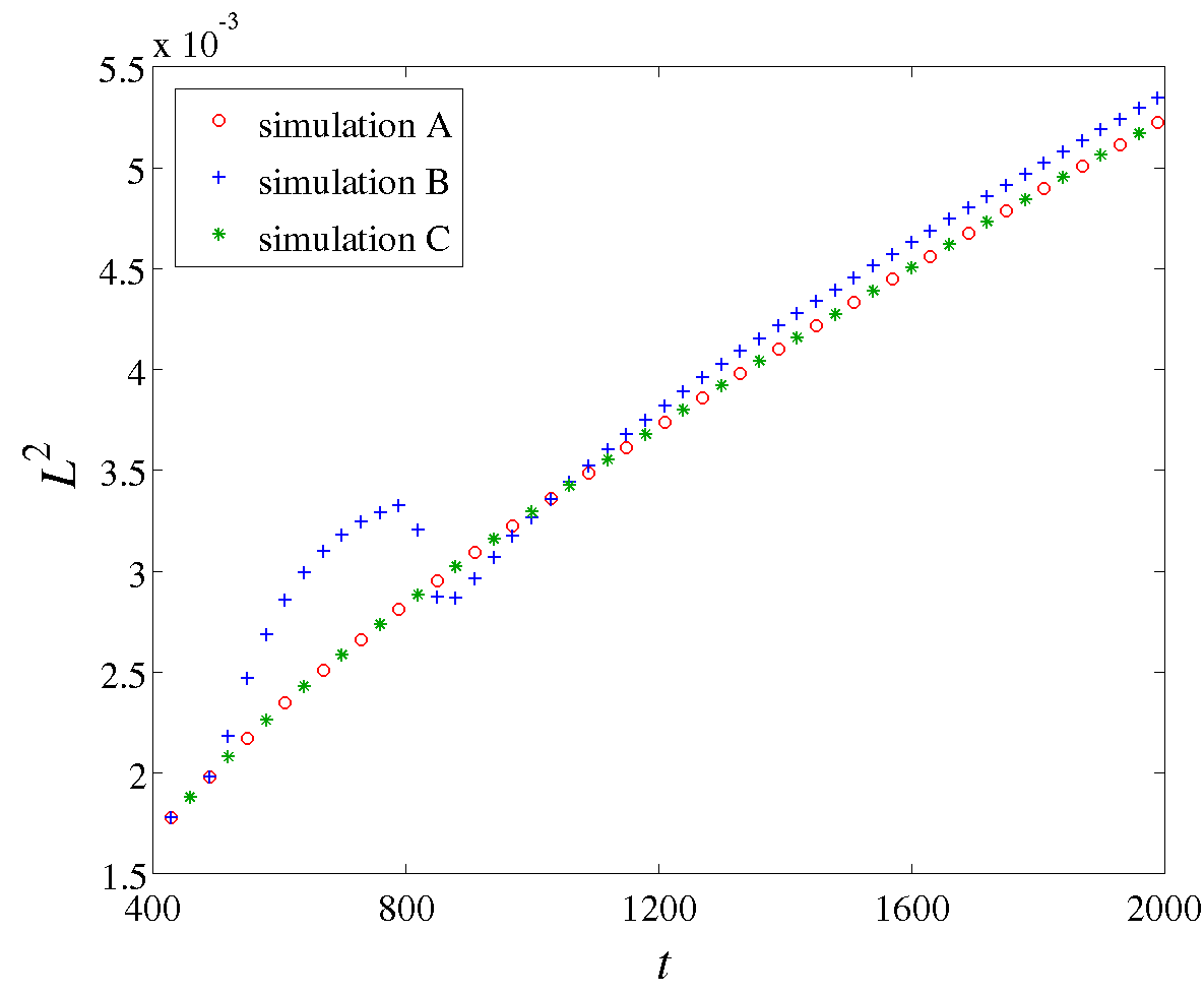
Figure 5: (Color online) Evolution of the characteristic length, $L(t)$, for simulations $A$, $B$ and $C$. Since the curves for simulations $A$ and $C$ are almost indistinguishable we intercalate the corresponding datapoints in order to improve the visualization.

Fig. 3 shows a snapshot of simulation $B$ for $t=900$ after the electric field has been rotated by an angle of $\pi$ and then switched off when at $t=800$. In this case, the components of the director are given by ${\bf n}=(n_{x_{0}},-n_{y_{0}},0)$ and all the half-integer disclinations are back into the $xy$ plane, with an opposite topological charge to the one they had in Figure 1. A similar realization of the exchange of sign of all half-integer disclinations network is possible through the rotation of the electric field around any other axis of the simulation plane. Besides this transformation of the topological charge, the electric field produces other effects on the network coarsening that need to be addressed in more detail.

In simulation $C$ we have implemented by hand the modification of the director and co-director profiles corresponding to a rotation of $\pi$ of an external electric field. This transformation was performed with the purpose of isolating the effect of the inversion of the sign of the half-integer disclinations from the modification of the coarsening dynamics associated with the presence of an external electric field. We have modified the components of ${\bf n}$ and ${\bf l}$ of the configuration at $t=500$, shown in Fig. 1, so that

$${n}_{x} = n_{x0}\,,\qquad{n}_{y}=-n_{y0}\,,$$

$${l}_{x} = n_{y0}\,,\qquad{l}_{y}=n_{x0}\,,$$ (16)

where ($n_{x_{0}}$, $n_{y_{0}}$, 0) are the components of the director ${\bf n}$ presented in Fig. 1. The results for the projection of the director onto the lattice plane are presented in Fig. 4 along with the order parameter $S$ for a snapshot of simulation $C$ at $t=900$. Fig. 4 is very similar to Fig. 1, except for the inversion of the sign of the topological charges and the coarsening which took place between $t=499$ and $t=900$.

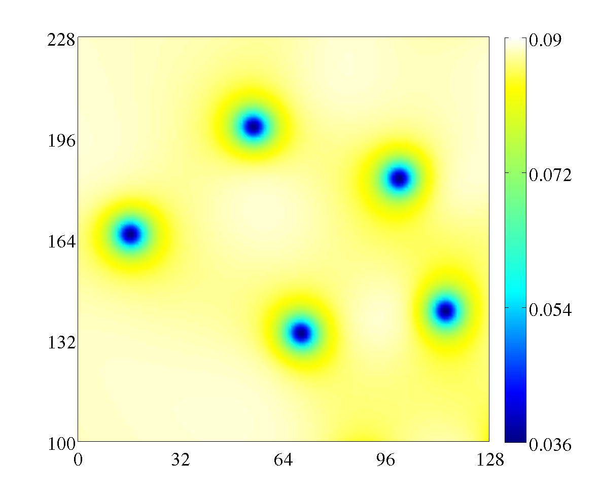
Figure 6: (Color online) Total free energy, given by Eq. (5), for a snapshot of simulation $A$ at $t=900$. The corresponding image for simulation $C$ is identical.

The evolution of the characteristic length, $L(t)$, of simulations $A$, $B$ and $C$ is presented in Figure 5. Given that the curves for simulations $A$ and $C$ are almost indistinguishable we intercalate the corresponding datapoints in order to improve the visualization. The effect of the rotation of the electric field is visible in simulation $B$, between $t=500$ and $t=800$. An acceleration of the coarsening, reflected in the larger slope of $L^{2}(t)$ may be observed between $t=500$ ($\varphi=0$) and $t=650$ ($\varphi=\pi/2$). It is also clear that the memory of the connection of the field is preserved by the coarsening dynamics in simulation $B$, even after the electric field is disconnected. This is reflected in the larger value of the characteristic length scale of the network at late time, compared to simulations $A$ and $C$.

The comparison of the evolution of $L^{2}(t)$ for simulations $A$ and $C$ demonstrates that modifying the director and co-director profiles by hand using Eq. (16) does not modify the coarsening dynamics. This happens because the bulk and elastic components of the free energy defined by Eqs. (6) and (7), are invariant by a rotation of the directors around an arbitrary axis. Such rotation originates a rotated director and co-director network profile with the same free energy at every point in space. This result can be confirmed in Fig. 6 which shows the total free energy, given by Eq. (5), for a snapshot of simulation $A$ at $t=900$ (the corresponding image for simulation $C$ is identical). As expected, the free energy profile is axially symmetric around the defect centers. Hence, the acceleration of the defect coarsening due to the application of an external electric field is associated with the modification of the degree of alignment of the molecules, reflected in the modification of the values of the order parameters $S$ and $T$, and it is therefore insensitive to the inversion of the sign of the topological charges.

V CONCLUSION

In this work we have numerically demonstrated that a rotation by $\pi$ of an external electric field around an axis of the plane of a 2D nematic liquid crystal induces an inversion of the sign of all half-integer disclinations, when a negative dielectric anisotropy is considered. We have further analysed the the impact of the exernal electric field on the coarsening dynamics.

The inversion of the topological charge investigated in the present paper may be realized experimentally in a simple setup. The topological arguments do not depend on the model parameters and apply to the different phases of a liquid crystal. Although we have assumed that the inversion was induced by the rotation of an external electric field, a magnetic field induced transition is also possible in the case of negative diamagnetic anisotropy.

References

- de Gennes and Prost (1995) P. G. de Gennes and J. Prost, The Physics of Liquid Crystals (Clarendon Press, Oxford, 1995), 2nd ed.
- Kleman and Lavrentovich (2003) M. Kleman and O. D. Lavrentovich, Soft Matter Physics: An Introduction (Springer, 2003).
- Vilenkin and Shellard (1994) A. Vilenkin and E. P. S. Shellard, Cosmic Strings and Other Topological Defects (Cambridge University Press, Cambridge, 1994).
- Chuang et al. (1991) I. Chuang, R. Durrer, N. Turok, and B. Yurke, Science 251, 1336 (1991), ISSN 0036-8075.
- Chuang et al. (1993) I. Chuang, B. Yurke, A. N. Pargellis, and N. Turok, Phys. Rev. E 47, 3343 (1993).
- Zapotocky et al. (1995) M. Zapotocky, P. M. Goldbart, and N. Goldenfeld, Phys. Rev. E 51, 1216 (1995).
- Digal et al. (1999) S. Digal, R. Ray, and A. M. Srivastava, Phys. Rev. Lett. 83, 5030 (1999).
- Denniston et al. (2001) C. Denniston, E. Orlandini, and J. M. Yeomans, Phys. Rev. E 64, 021701 (2001).
- Dutta and Roy (2005) S. Dutta and S. K. Roy, Phys. Rev. E 71, 026119 (2005).
- de Lózar et al. (2005) A. de Lózar, W. Schöpf, I. Rehberg, D. Svenšek, and L. Kramer, Phys. Rev. E 72, 051713 (2005).
- Mukai et al. (2007) H. Mukai, P. R. G. Fernandes, B. F. de Oliveira, and G. S. Dias, Phys. Rev. E 75, 061704 (2007).
- Bhattacharjee et al. (2008) A. K. Bhattacharjee, G. I. Menon, and R. Adhikari, Phys. Rev. E 78, 026707 (2008).
- Kitzerow (1991) H. S. Kitzerow, Mol. Cryst. Liq. Cryst. 202, 51 (1991).
- Dierking et al. (2005) I. Dierking, O. Marshall, J. Wright, and N. Bulleid, Phys. Rev. E 71, 061709 (2005).
- Alexander and Marenduzzo (2008) G. P. Alexander and D. Marenduzzo, EPL 81, 66004 (2008).
- Fukuda et al. (2009) J.-i. Fukuda, M. Yoneya, and H. Yokoyama, Phys. Rev. E 80, 031706 (2009).
- Fukuda (2010) J.-i. Fukuda, Phys. Rev. E 81, 040701 (2010).
- de Oliveira et al. (2010) B. F. de Oliveira, P. P. Avelino, F. Moraes, and J. C. R. E. Oliveira, Phys. Rev. E 82, 041707 (2010).
- de Gennes (1971) P. G. de Gennes, Mol. Cryst. Liq. Cryst. 12, 193 (1971).