Dissimilar bouncy walkers

Abstract

We consider the dynamics of a one-dimensional system consisting of dissimilar hardcore interacting (bouncy) random walkers. The walkers’ (diffusing particles’) friction constants $\xi_{n}$, where $n$ labels different bouncy walkers, are drawn from a distribution $\varrho(\xi_{n})$. We provide an approximate analytic solution to this recent single-file problem by combining harmonization and effective medium techniques. Two classes of systems are identified: when $\varrho(\xi_{n})$ is heavy-tailed, $\varrho(\xi_{n})\simeq\xi_{n}^{-1-\alpha}\ (0<\alpha<1)$ for large $\xi_{n}$, we identify a new universality class in which density relaxations, characterized by the dynamic structure factor $S(Q,t)$, follows a Mittag-Leffler relaxation, and the the mean square displacement of a tracer particle (MSD) grows as $t^{\delta}$ with time $t$, where $\delta=\alpha/(1+\alpha)$. If instead $\varrho$ is light-tailed such that the mean friction constant exist, $S(Q,t)$ decays exponentially and the MSD scales as $t^{1/2}$. We also derive tracer particle force response relations. All results are corroborated by simulations and explained in a simplified model.

I Introduction

The staggering motion of a lone drunk has, since the classic correspondence Pearson ; Lord_Rayleigh between Karl Pearson and Lord Rayleigh in 1905, been a well established metaphor for a random walk. This view was embraced in a celebrated work Fisher_84 by Michael E. Fisher in which he discussed statistical aspects of many drunks. In particular, Fisher introduced the notion of harmless drunks for identical non-interacting walkers, vicious drunks representing the motion of antagonists, and bouncy walkers exhibiting hardcore repulsive interactions in one dimension.

The bouncy walker problem, which we here revisit, finds a number of experimental realizations: transport in microporous materials KKDGPRSUK ; meersmann00 ; hahn96 (e.g. zeolites), colloidal systems WBL , molecular sieves gupta95 and biological pores HOKE . Hard core repulsion of binding proteins diffusing along DNA was recently suggested to be important in transcription. Elf_09

On the theoretical side, the many-body problem of identical bouncy walkers in one dimension, also referred to as single-file diffusion LE or symmetric exclusion Arratia_83 , has received considerable attention since it was introduced by HarrisHA in 1965. The main result for thermal initial conditions is that a tracer particle exhibits sub-diffusion LE ; HA ; Alexander_Pincus_78 ; Kollmann_03 ; barkai2009theory ; the tracer mean square displacement (MSD) is proportional to $t^{1/2}$ even though the collective behavior is diffusive (the structure factor $S(Q,t)$ decays exponentially LIAM2 ). In this study, we ask: what are corresponding expressions for the MSD and $S(Q,t)$ for a system of dissimilar bouncy walkers? We show that this question can be answered in closed form, using harmonization lizana_10 and effective medium approaches landauer52 ; kirkpatrick71 ; alexander81 . The analytic predictions are corroborated by extensive simulations. Our results extend, in ways described throughout the study, a very limited number of previous studies Jara_Gonzalves ; TA_etal ; Jara_09 ; Flomenbom of bouncy walkers of different type.

II Equations of motion

We consider strongly overdamped motion of Brownian particles, in an infinite one dimensional system, interacting via a two-body short-range repulsive potential. The nearest neighbor potential ${\cal V}(|x_{n}(t)-x_{n^{\prime}}(t)|)$, where $x_{n}(t)$ is the position of the $n$th particle, has a hard-core part which excludes particles from overtaking each other. The Langevin equations of motion are thus

$$\xi_{n}\dot{x}_{n}(t)=\sum_{n^{\prime}}\mathfrak{f}[x_{n}(t)-x_{n^{\prime}}(t)]+\eta_{n}(t)+f_{n}(t),$$ (1)

where a dot denotes time derivative, $\mathfrak{f}=-\partial{\cal V}/\partial x_{n}$, $\eta_{n}(t)$ is a Gaussian zero-mean noise, $\mathbf{<}\eta_{n}(t)\mathbf{>}=0$, with correlations that are determined by the fluctuation-dissipation theorem kubo66 to be $\mathbf{<}\eta_{n}(t)\eta_{n^{\prime}}(t^{\prime})\mathbf{>}=2k_{B}T\xi_{n}\delta(t-t^{\prime})\delta_{n,n^{\prime}}$, where $k_{B}$ is the Boltzmann constant and $T$ the temperature. $f_{n}(t)$ is an external force and particle $n$ has the friction constant $\xi_{n}$. In Sec. IV where the system’s collective behavior is considered we take $f_{n}(t)\equiv 0$. At the end of Sec. V and in Sec. VI we assume $f_{n}(t)$ to be a static force turned on at $t=0$ or an oscillating force acting only on the tracer particle.

The dissimilarity of the random walkers enter through their different friction constants, $\xi_{n}$, which here are assumed to be identically distributed random variables taken from a probability density $\varrho(\xi_{n})$. Eq. (1), the noise correlation and $\varrho(\xi_{n})$ defines the dissimilar bouncy walkers problem which we deal with by using two non-equilibrium statistical physics methods outlined below and elaborated in appendix A.

We complement all analytic results by stochastic simulations for hardcore interacting particles in a box with reflecting boundary conditions, detailed in appendix G. The box size is chosen sufficiently large such that boundary effects are negligible for the center particle within the duration of the simulation run.

A prototypical system where Eq. (1) is applicable is protein diffusion on DNA moleculesElf_09 , where the heterogeneity in friction constants originate from the different proteins varying binding strength to the DNA molecule.

III Harmonization and effective medium theory

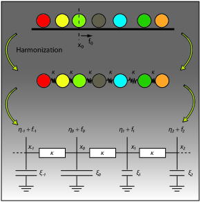
Figure 1: Two mappings bring the bouncy walker problem (top) on a tractable form. Harmonization maps the system onto that of harmonically coupled, Rouse chain type Khokhlov , beads (middle). The corresponding Eq. (2) has the same form as the equation appearing in resistor-capacitor network theory where $x_{n}$ represent the node potentials, $\xi_{n}$ are capacitances, $\kappa$ is the conductance of the resistors and $\eta_{n}+f_{n}$ is an external current entering the circuit at node $n$ (bottom). This analogy allow us to derive an effective medium Eq. (3) of the type originally used to calculate conductances of binary metallic mixtures landauer52 and later extended to resistor networks kirkpatrick71 and applied to diffusion in random media alexander81 .

Our first step towards bringing the dissimilar walker problem on a tractable form is to generalize the harmonization approach lizana_10 to the case when the particles have different friction constants. In the long time limit this allows us to map the equations of motion (1) onto that for a linear chain of interconnected springs

$$\xi_{n}\frac{dx_{n}(t)}{dt}=\kappa\left[x_{n+1}(t)+x_{n-1}(t)-2x_{n}(t)\right]+\eta_{n}(t)+f_{n}(t),$$ (2)

corresponding to harmonically coupled beads, see Fig. 1. The effective nearest neighbor spring constant $\kappa$ is calculated by demanding that the change in free energy for small particle displacements in the original system equals the free energy change in the spring system. For hardcore interacting particles of size $b$ (used in our simulations) this harmonization procedure yields lizana_10 $\kappa=\rho^{2}k_{B}T(1-\rho b)^{-2}$, where $\rho$ is the particle density. The harmonization approach relies on the assumption that local equilibration is faster than tracer particle dynamics, for sufficiently long times. We find self-consistently that this holds since, as we will see, the MSD for a single particle is proportional to $t^{\delta}$ with $\delta\leq 1/2$ [see Eq. (11)], i.e., the particle cross a distance of length $L$ in a time on the order of $L^{2/\delta}$. At long distances this is indeed slower than the corresponding density relaxation time which scales as $L^{1/\delta}$ [see Eq. (9)].

Second, applying an effective medium approach landauer52 ; kirkpatrick71 ; alexander81 to the harmonized equations yields a set of generalized Langevin equations containing a time dependent, but $n$ independent, memory kernel $\xi_{\rm eff}(t)$. This method is based on an analogy of our system with that of resistor networks, see Fig. 1. In the continuum limit (in the long-wavelength limit $n$ can be treated as a continuum variablelizana_10 ) the effective medium harmonized equations are

$$\int_{-\infty}^{\infty}\xi_{\rm eff}(t-t^{\prime})\dot{x}_{n}(t^{\prime})\,dt^{\prime}=\kappa\frac{\partial^{2}x_{n}(t)}{\partial n^{2}}+\eta_{n}^{\rm eff}(t)+f_{n}(t).$$ (3)

The lower integration limit being $-\infty$ physically corresponds to the system dynamics being “turned on” in the infinite past, thereby effectively bring the system to equilibrium at any finite time $t$. As shown below $\xi_{\rm eff}(t-t^{\prime})=0$ for $t^{\prime}>t$, as required by causality. The fluctuation-dissipation theorem enforces a relation between the memory kernel and the effective noise $\eta_{n}^{\rm eff}(t)$ kubo66 :

$$\left<\eta_{n}^{\rm eff}(t)\eta_{n^{\prime}}^{\rm eff}(t^{\prime})\right>=k_{B}T\xi_{\rm eff}(|t-t^{\prime}|)\delta(n-n^{\prime}),$$ (4)

where the brackets $\langle..\rangle$ represent an implicit average over quenched friction constants, besides averages over different realization of the noise and random initial positions. We label this average the heterogeneity-averaged case Jara_Gonzalves , which is contrasted by the non-averaged case (represented by $\mathbf{<}..\mathbf{>}$) where an average over the probability density of friction constants is not performed. In the simulations for the non-averaged case the same $\xi_{n}$’s are used when averaging over thermal noise (i.e., for each simulation run). For the heterogeneity averaged case we draw new friction constants whenever we make a new initial particle positioning.

The memory kernel, $\xi_{\rm eff}(t)$, in Eq. (3) is determined by imposing a self-consistency criterion (see appendix A). We identify two classes of systems: For light-tailed (LT) systems with a probability density $\varrho(\xi)$ such that the mean friction $\bar{\xi}=\int_{0}^{\infty}\xi\varrho(\xi)d\xi$ exists, we obtain, in the long time limit, a memoryless kernel

$$\xi_{\rm eff}(t)\sim{\bar{\xi}}\delta(t),$$ (5)

where $\delta(z)$ is the Dirac delta-function. Thus, LT systems are in the same universality class as that of identical bouncy walkers lizana_10 . In contrast, we find that heavy-tailed (HT) systems, where $\varrho(\xi)=A\xi^{-1-\alpha}$ for large $\xi$, with $0<\alpha<1$ ($A$ is a normalization constant), belong to a new universality class where the memory kernel has a power-law decay with time

$$\xi_{\rm eff}(t)\sim\chi\frac{t^{-2\delta}}{\Gamma(1-2\delta)}\theta(t)$$ (6)

where $\Gamma(z)$ is the gamma function, $\theta(z)$ is the Heaviside step function, $\chi=(4\kappa)^{1-2\delta}(A\pi/\sin[\delta\pi/(1-\delta)])^{2(1-\delta)}$ and

$$\delta=\frac{\alpha}{1+\alpha}.$$ (7)

We point out that for HT systems it is only the tail of the distribution [the detailed structure of $\varrho(\xi)$ for small $\xi$ is not important] which determines the long-time dynamics. The equations (3)-(6) in this section allow us to calculate explicit long-time expressions for observables in dissimilar bouncy walker systems [i.e., systems described by Eq. (1)].

IV Collective behavior

Let us now consider the collective behavior of dissimilar bouncy walker systems, using the analytic approach in Sec. III and the simulation scheme from appendix G. A quantity capturing the collective motion and easily accessible in experiments Berne_Pekora is the dynamic structure factor $S(Q,t)$. For translationally invariant systems we use $S(Q,t)=\sum_{n}\langle e^{iQ[x_{n}(t)-x_{0}(0)]}\rangle$ where the summation index runs over all particles. For LT systems we find from Eq. (3) (see appendix C), in the limit of small wavevectors $Q\neq 0$ and long times, that

$$S(Q,t)\sim S(Q,0)\exp(-D_{c}Q^{2}t)$$ (8)

with the static structure factor $S(Q,0)=k_{B}T\rho^{2}/\kappa$ and the collective diffusion constant $D_{c}=\kappa/(\rho^{2}\bar{\xi})$. Density relaxations are thus exponential as for a system of harmless drunks Berne_Pekora or identical bouncy walkers TA_etal . For HT systems we find a collective behavior which is drastically different:

$$S(Q,t)\sim S(Q,0)E_{2\delta}(-\lambda_{c}Q^{2}t^{2\delta}),\qquad Q\neq 0$$ (9)

where $E_{\alpha}(z)$ is the Mittag-Leffler function MEKL1 and $\lambda_{c}=\kappa/(\rho^{2}\chi)$ is a generalized collective diffusion constant. Here, the density relaxations exhibit anomalously slow power-law decay with time. The anomalous decay of $S(Q,t)$ is illustrated in Fig. 2 together with simulation results for the non-averaged case.

From Eq. (9) and Onsager’s regression hypothesis onsager31 it follows that perturbations of the concentration $c(X,t)=\langle\sum_{m}\delta(X-x_{m}(t))\rangle$ around its equilibrium value $\rho$ decay according to the fractional diffusion equation $\partial c(X,t)/\partial t=\lambda_{c}D^{1-2\delta}_{t}\partial^{2}c(X,t)/\partial X^{2}$ where ${}_{0}D^{1-2\delta}_{t}$ is the fractional Riemann-Liouville operator. This equation describes also the subdiffusive motion of non-interacting continuous time random walkers (CTRW) with a power-law waiting time density MEKL1 . However, the nature of the process is here very different. In particular, our system has a stationary fluctuating equilibrium state, since the underlying many-body dynamics is Markovian with a well-defined equilibrium (two point correlation functions only depend on the time difference, i.e., the system do not age). In contrast, CTRWs do not have a stationary state (their two point correlation functions age). Therefore, to the best of our knowledge, dissimilar bouncy walkers are the first example of a stationary physical system obeying (to a good approximation) the fractional diffusion equation for density relaxations. The fact that our HT bouncy walkers belong to a different universality class than CTRW systems is also captured by the difference in tracer particle behavior.

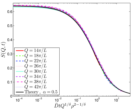
Figure 2: Dynamic structure factor. Collapse-plot for $S(Q,t)$ for different wavevectors $Q$ as a function of time, illustrating anomalous decay. The black solid curve is the analytic prediction, Eq. (9). Simulations are non-averaged results from 32000 noise realizations with $N=501$ particles in a system of length L=2501b ($b$ is the particle size) with $\alpha=0.5$. The average diffusion constant is denoted $\bar{D}$. Note that, in contrast to tracer particle observables (see inset of Fig. 3) $S(Q,t)$ is a sum over all particles and therefore display self-averaging.

V Tracer particle dynamics, heterogeneity-averaged case

We now address tracer particle dynamics in the absence of an external force (see appendix D for details) using Eqs. (3)-(6) . For LT systems we find the MSD

$$\langle\delta x_{\mathcal{T}}^{2}(t)\rangle\sim k_{B}T\sqrt{\frac{4t}{\pi\kappa\bar{\xi}}}\propto t^{1/2},$$ (10)

for particle $\mathcal{T}(=0)$. Thus, the MSD for LT systems take the same form as for identical walkerslizana_10 , but with the friction constant for the homogeneous case replaced by the mean friction constant $\bar{\xi}$. The same $t^{1/2}$-scaling was recently obtained for dissimilar walkers on a lattice. Jara_Gonzalves ; TA_etal A very different MSD exponent is found for HT systems where instead

$$\langle\delta x_{\mathcal{T}}^{2}(t)\rangle\sim\frac{k_{B}T}{\sqrt{\kappa\chi}}\frac{t^{\delta}}{\Gamma(1+\delta)}\propto t^{\delta}$$ (11)

with $\delta<1/2$ [see Eq. (7)] indicating ultra-slow dynamics for the tracer particle. Heterogeneity-averaged simulations show excellent agreement with this result, see Fig. 3. The MSD exponent $\delta=\alpha/(1+\alpha)$ has also recently been derived for lattice systems in a rather technical mathematical study by Jara Jara_09 and obtained through scaling arguments in Ref. Flomenbom, . Besides providing a simplified derivation for continuum systems, we extend Jara’s result by also obtaining an explicit expression for the MSD prefactor. The probability density function (PDF) for the tracer particle position is a Gaussian (since the noise is taken from a multi-variate normal distribution) with a width described by Eq. (11), see appendix G for corroborating simulations.

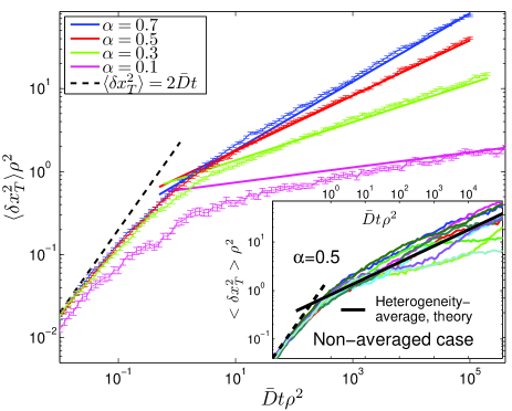
Figure 3: Tracer particle mean square displacement. MSD as a function of time for the heterogeneity-averaged and non-averaged (inset) cases. The straight solid lines are the asymptotic analytic prediction, Eq. (11), and the dashed lines are the result for an independent random walker. In the heterogeneity-averaged case the simulations are averages over 2400 realizations, and the center particle is taken as tracer particle. We used a box size $L=10001b$ ($b$ is the particle size) and $N=1001$ particles for $\alpha=0.7$ and $\alpha=0.5$. For $\alpha=0.3$ ($\alpha=0.1$) we had $N=501$ and $L=5001b$ ($N=251$ and $L=2501b$). The average diffusion constant is $\bar{D}$. Inset: Non-averaged MSD simulations for $\alpha=0.5$ and 800 noise realizations for each curve. Notice the spread around the analytic result.

In the presence of a external force on the tracer particle we calculate force-response relations (see Appendices E and F). For the case of a static force $f_{n}(t)=\delta_{n,0}F_{0}\theta(t)$ with magnitude $F_{0}$, we show by explicit calculation that the generalized Einstein relation $\langle x_{\mathcal{T}}(t)\rangle_{f}=\langle\delta x_{\mathcal{T}}^{2}(t)\rangle F_{0}/(k_{B}T)$ is satisfied for both LT and HT systems. The bracket $\langle..\rangle_{f}$ denotes an average in the presence of $f_{n}(t)$. For an oscillatory force $f_{n}(t)=\delta_{n,0}F_{0}\cos(\omega_{0}t)$ with angular velocity $\omega_{0}$ we get $\langle x_{\mathcal{T}}(t)\rangle_{f}=[F_{0}/(2\sqrt{\kappa\bar{\xi}\omega_{0}})]\cos(\omega_{0}t-\phi)$ where $\phi=\pi/4$ for LT systems. For HT systems we find

$$\langle x_{\mathcal{T}}(t)\rangle_{f}=\frac{F_{0}}{2\sqrt{\kappa\chi}\omega_{0}^{\delta}}\cos(\omega_{0}t-\phi)$$ (12)

with the non-trivial phase-shift $\phi=\delta\pi/2<\pi/4$, which compactly quantifies the subtle interplay between bounciness and the degree of friction dissimilarity. Eq. (12) is compared to simulations for the heterogeneity-averaged case in Fig. 4.

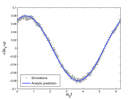
Figure 4: Mean displacement for a tracer particle in the presence of a time-varying force. Simulations for the average displacement of a tracer particle as a function of time within a single period of a harmonically oscillating external force, heterogeneity-averaged case. Parameters are $\alpha=0.5$, $N=501$, $L=5001b$ ($b$ is the particle size), $\alpha_{0}=0.002$ and $\omega_{0}/(2\pi)=10^{-5}$. The average is over last 100 periods of the force for 1280 noise realizations each lasting 200 periods. The blue solid curve is the analytic prediction, Eq. (12). Notice the excellent agreement between theory and simulations.

VI Self-averaging

Let us comment on the difference between the non-averaged and heterogeneity-averaged cases. From simulations for both cases we found that $S(Q,t)$ and the MSD are self-averaging quantities for the LT class, as has been previously shown for lattice systems Jara_Gonzalves ; TA_etal . For HT systems $S(Q,t)$ self-averages while the MSD does not (see Figs. 2 and 3). In order to understand this in more detail, we put forward a simplified model for tracer particle dynamics in the non-averaged case: under the influence of a constant force, $F_{0}$, we write $\xi_{\rm tot}d\mathbf{<}\delta x_{\mathcal{T}}\mathbf{>}_{F_{0}}/dt=F_{0}$. We use brackets $\mathbf{<}..\mathbf{>}$ to denote averages over thermal noise and random initial positions for the non-averaged case. The quantity $\xi_{\rm tot}$ represents the total friction experienced by the particle which is not only its own, but also that of an approximate number $N$ of its neighbors on which it is “pushing”, i.e. $\xi_{\rm tot}=\xi_{0}+\xi_{1}+\xi_{2}+...+\xi_{N}$. Within the harmonization approach lizana_10 we have approximately that the effective spring constant for $N$ serially connected springs is $\kappa/N$, i.e., we have $F_{0}=(\kappa/N)\mathbf{<}\delta x_{\mathcal{T}}\mathbf{>}_{F_{0}}$, from which $N=\kappa\mathbf{<}\delta x_{\mathcal{T}}\mathbf{>}_{F_{0}}/F_{0}$; the larger the displacement the larger is the number of particles contributing to $\xi_{\rm tot}$. Using this result and multiplying and dividing the equation of motion above by $N^{1/\alpha}$ we arrive at

$$\underbrace{\frac{\xi_{1}+\xi_{2}+...+\xi_{N}}{N^{1/\alpha}}}_{\zeta}(\kappa\mathbf{<}\delta x_{\mathcal{T}}\mathbf{>}_{F_{0}}/F_{0})^{1/\alpha}\frac{d\mathbf{<}\delta x_{\mathcal{T}}\mathbf{>}_{F_{0}}}{dt}=F_{0},$$

where $\zeta$ is a random variable with an $N$-independent distribution $\psi(\zeta)$ for $N\rightarrow\infty$. Solving the equation above and employing the fluctuation-dissipation theorem in the form of the generalized Einstein relation, $k_{B}T\mathbf{<}\delta x_{\mathcal{T}}\mathbf{>}_{F_{0}}/F_{0}=\mathbf{<}\delta x_{\mathcal{T}}^{2}\mathbf{>}$, we find the MSD for the non-averaged case:

$$\mathbf{<}\delta x_{\mathcal{T}}^{2}\mathbf{>}\propto\frac{k_{B}T}{\zeta^{\delta}\kappa^{1-\delta}}t^{\delta}.$$ (13)

In agreement with the non-averaged case simulations (inset Fig. 3), the MSD prefactor is a random variable $\zeta$. Thus, HT systems do not show self-averaging, rather each new realization of $\xi_{n}$’s gives a different fluctuating prefactor for the MSD (but with the same scaling with time). The very simplistic argument here predicts that for HT systems $\psi(\zeta)$ is a one-sided Lévy stable distribution MEKL1 , but further work is needed to pinpoint the correct functional form for $\psi(\zeta)$. We point out that the non-averaged HT case has not been investigated in previous studies Jara_09 . Using the fact that $\langle\zeta^{-\delta}\rangle\propto A^{-(1-\delta)}$ for the power-law distribution of friction constants considered here, our simplified model recovers Eq. (11), up to a dimensionless $\alpha$-dependent prefactor for the heterogeneity-averaged case. For LT systems ($\alpha=1$) the central limit theorem gives $\psi(\zeta)=\delta(\zeta-\bar{\xi})$ as $N\rightarrow\infty$, i.e., the argument above predicts that LT systems possess the self-averaging property as indeed found in our simulations.TA_etal

VII Summary and outlook.

We investigated the dynamics of a one-dimensional system consisting of dissimilar bouncy random walkers, with friction constants drawn from a probability density. Two classes of systems were identified: those with heavy-tailed (HT) probability densities in which density relaxations, characterized by the dynamic structure factor $S(Q,t)$, follows a Mittag-Leffler relaxation. The mean square displacement of a tracer particle (MSD) grows as $t^{\delta}$ with time $t$, where $\delta<1/2$, and we find a phase-shift $\phi=\delta\pi/2$ in the force-response relation for such systems. For light-tailed (LT) probability densities, $S(Q,t)$ decay exponentially, the MSD scales as $t^{1/2}$ and a phase-shift $\phi=\pi/4$ in the force response is obtained. We also introduced a simplified model which allowed us to address the problem of self-averaging for LT and HT systems. All results were corroborated by extensive simulations.

Prior to this study, dissimilar hardcore interacting diffusing particles have been investigated only in a few publications, see Refs. Jara_Gonzalves, ; TA_etal, ; Flomenbom, ; Jara_09, . Using harmonization and effective medium approaches we here extended previous results by providing: (i) an explicit expression for the structure factor $S(Q,t)$; (ii) an explicit prefactor for the MSD for HT systems; (iii) force-response relations for a tracer particle; (iv) insights concerning the difference between non-averaged and heterogeneity-averaged cases for HT systems; (v) extensive simulation results. We further provided a much simplified framework, Eqs. (3)-(6), within which further observables, such as correlation functions between particles (see Ref. lizana_10, ), can be calculated.

Solvable many-body problems have served as important models for real systems over the last century. The problem of dissimilar bouncy walkers is expected to find applications in systems such as passive diffusion of proteins along DNA or particles diffusing in nanochannels. Further, often the dynamics of macromolecules in living cells is found to be subdiffusive weiss_09 . The techniques developed in this study may be of use also in such higher dimensional heterogeneous systems.

VIII Acknowledgment

We are grateful to Mehran Kardar and Eli Barkai for discussions and Milton Jara for helpful correspondence regarding Ref. Jara_09, . T.A. and L.L. acknowledges funding from the Knut & Alice Wallenberg Foundation. T.A. is grateful for funding from the Swedish Research Council. Computer time was provided by the Danish Center for Scientific Computing.

Appendix A Effective medium approach.

Our second step in deriving a set of manageable equations for the dissimilar bouncy walker problem is to introduce an effective medium approximation known for instance from the theory of resistor networks kirkpatrick73 , see Fig. 1. In the language of single-file motion the approximation consists of replacing the different frictions $\xi_{n}$ in Eq. (2) with an effective friction, or memory kernel, $\xi_{\rm eff}(t)$, which is identical for all the particles, but instead has a memory. The memory kernel $\xi_{\rm eff}(t)$ is chosen such that if one takes a random particle from the harmonized system with friction constant $\xi_{n}$ and place it among particles characterized by $\xi_{\rm eff}(t)$, then the mobility of this particle is, on average [averaged using $\varrho(\xi_{n})$], required to be identical to the mobility of a tracer particle in the system where all particles had friction $\xi_{\rm eff}(t)$. A detailed calculation of $\xi_{\rm eff}(t)$ is given below.

Let us, as our starting point, consider the harmonized equation (2), which we write:

$$\xi_{n}\frac{dy_{n}(t)}{dt}=\kappa\left[y_{n+1}(t)+y_{n-1}(t)-2y_{n}(t)\right]+\eta_{n}(t)+f_{n}(t)$$ (14)

where we introduced $y_{n}(t)=x_{n}(t)-n\rho^{-1}$, which eliminates the average values so that $\mathbf{<}y_{n}(t)\mathbf{>}=0$. Our goal here is to find the friction kernel $\xi_{\rm eff}(t)$ entering the effective medium harmonization equation of motion

$$\int_{-\infty}^{\infty}\xi_{\rm eff}(t-t^{\prime})\frac{dy_{n}(t^{\prime})}{dt^{\prime}}dt^{\prime} = \kappa\left[y_{n+1}(t)+y_{n-1}(t)-2y_{n}(t)\right]$$ (15)

$$+\eta_{n}^{\rm eff}(t)+f_{n}(t)$$

which in the continuum limit with respect to $n$ becomes Eq. (3) in the main text. We introduce the frequency-dependent generalized friction constants

$$\gamma^{(\pm)}_{n}(\omega)\equiv-\frac{F_{n\pm 1\to n}(\omega)}{\mathbf{<}v_{n}(\omega)\mathbf{>}}$$ (16)

where $v_{n}(\omega)=-i\omega y_{n}(\omega)$ is the Fourier transform of the velocity, and $F_{n\to n+1}=-\kappa(y_{n+1}-y_{n})$ is the force from particle $n$ on particle $n+1$ within the harmonization approach. The quantity $\gamma^{(+)}_{n}$ ($\gamma^{(-)}_{n}$) can be thought of as a generalized friction of particle $n$ due to the part of the harmonic chain lying to right (left) of particle $n$. We here define the Fourier-transform with respect to time of a function $A(t)$ according to: $A(\omega)=\int_{-\infty}^{\infty}e^{i\omega t}A(t)dt$, with inverse transform $A(t)=\int_{-\infty}^{\infty}e^{-i\omega t}A(\omega)d\omega/(2\pi)$. Using the generalized frictions introduced above and setting $f_{n}(t)=f_{0}(t)\delta_{n,0}$ one readily obtains, from the Fourier-transform of Eq. (2), the mobility of particle 0

$$\mu_{0}(\omega)\equiv\frac{\langle v_{0}(\omega)\rangle}{f_{0}(\omega)}=\frac{1}{\xi_{0}+\gamma^{(+)}_{0}(\omega)+\gamma^{(-)}_{0}(\omega)},$$ (17)

as well as the recursion relations

$$\gamma^{(+)}_{n}(\omega)=\frac{\xi_{n+1}+\gamma^{(+)}_{n+1}(\omega)}{1-i\omega\left[\xi_{n+1}+\gamma^{(+)}_{n+1}(\omega)\right]/\kappa}\;,\quad n\geq 0$$ (18)

and

$$\gamma^{(-)}_{n}(\omega)=\frac{\xi_{n-1}+\gamma^{(-)}_{n-1}(\omega)}{1-i\omega\left[\xi_{n-1}+\gamma^{(-)}_{n-1}(\omega)\right]/\kappa}\;,\quad n\leq 0$$ (19)

So far everything is only a reformulation of Eq. (14) for the case $f_{n}(t)=f_{0}(t)\delta_{n,0}$. We point out that we could equally well have reformulated Eq. (14) by using Laplace-transformed quantities $A(s)=\int_{0}^{\infty}e^{-st}A(t)dt$; the corresponding recursion relations would then take the same form as in Eqs. (18) and (19), with $s=-i\omega$. However, for the purpose of avoiding to explicitly compute averages over initial positions using Fourier-transforms is more convenient, and we therefore employ Fourier-transform techniques throughout this study.

Let us now turn to the problem of computing $\xi_{\rm eff}(t)$ in the effective medium Eq. (15). We invoke the following procedure: (A) Fourier-transform Eq. (14), and replace all friction constants for $n\neq 0$ by an $n$ independent but frequency dependent effective friction, i.e. we let

$$\xi_{n}\rightarrow(1-\delta_{n,0})\xi_{\rm eff}(\omega)+\xi_{0}\delta_{n,0}.$$ (20)

From these equations the mobility $\mu_{0}(\xi_{0})$ for particle $0$ is determined. (B) We then obtain $\xi_{\rm eff}(\omega)$ by imposing the self-consistency requirement that $\mu_{0}(\xi_{0})$ averaged over different realizations of $\xi_{0}$,

$$\bar{\mu}_{0}=\int_{0}^{\infty}\mu_{0}(\xi_{0})\varrho(\xi_{0})d\xi_{0},$$ (21)

is equal to the tracer particle mobility, $\mu_{\rm eff}(\omega)$, obtained from the effective medium Eq. (15), i.e., when also $\xi_{0}$ is replaced by $\xi_{\rm eff}(\omega)$.

Let us now carry out the scheme above. (A) From Eqs. (18), (19) and (20)

$$\gamma_{\rm eff}=\frac{\xi_{\rm eff}+\gamma_{\rm eff}}{1-i\omega\left[\xi_{\rm eff}+\gamma_{\rm eff}\right]/\kappa}.$$ (22)

where we left arguments implicit, and $\gamma_{\rm eff}=\gamma^{(+)}_{n}=\gamma^{(-)}_{n}$ (independent of $n$). Thus,

$$\gamma_{\rm eff}=-\frac{\xi_{\rm eff}}{2}+\Big{(}\frac{\kappa\xi_{\rm eff}}{-i\omega}\Big{)}^{1/2}\Big{(}1-\frac{i\omega\xi_{\rm eff}}{\kappa}\Big{)}^{1/2},$$ (23)

where we used the fact that the real part of $\gamma_{\rm eff}$ needs to be positive (so the friction will dissipate energy) to choose the correct root of the quadratic Eq. (22). For small frequencies (long times) we have

$$\gamma_{\rm eff}\sim\Big{(}\frac{\kappa\xi_{\rm eff}}{-i\omega}\Big{)}^{1/2}.$$ (24)

(B) From the self-consistency criterion we now determine $\xi_{\rm eff}$. Setting $n=0$ in Eqs. (18) and (19) we obtain the generalized friction $\gamma_{0}^{(\pm)}=(\xi_{\rm eff}+\gamma_{\rm eff})/(1-i\omega\left[\xi_{\rm eff}+\gamma_{\rm eff}\right]/\kappa)$ for particle 0. Combining this result with Eqs. (17), (21) and the self-consistency criterion, $\bar{\mu}_{0}=\mu_{\rm eff}(\omega)$, we get:

$$\int_{0}^{\infty}\frac{\varrho(\xi_{0})d\xi_{0}}{\xi_{0}+2\gamma_{\rm eff}}=\frac{1}{\xi_{\rm eff}+2\gamma_{\rm eff}}$$ (25)

where the right-hand side is the mobility obtained through the effective medium equations [simply replace $\xi_{0}\rightarrow\xi_{\rm eff}$ and $\gamma_{0}^{(\pm)}\rightarrow\gamma_{\rm eff}$ in Eq. (17)]. Eq. (25) can be rewritten:

$$\xi_{\rm eff}\int_{0}^{\infty}\frac{\varrho(\xi_{0})d\xi_{0}}{\xi_{0}+2\gamma_{\rm eff}}=\int_{0}^{\infty}\xi_{0}\frac{\varrho(\xi_{0})d\xi_{0}}{\xi_{0}+2\gamma_{\rm eff}}$$ (26)

where the normalization condition $1=\int_{0}^{\infty}\varrho(\xi_{0})d\xi_{0}$ was used. To summarize briefly, the effective friction $\xi_{\rm eff}(\omega)$ is uniquely determined by Eqs. (23) [Eq. (24) for small frequencies)] and (26) for a given choice of $\varrho(\xi_{0})$.

Now we have to distinguish two cases: (LT) the distribution $\varrho(\xi_{0})$ has a finite first moment, $\bar{\xi}=\int\xi_{0}\varrho(\xi_{0})d\xi_{0}<\infty$. In this case the $\xi_{0}$’s in the denominators on both sides of Eq. (26) can be discarded for large $\omega$ since we expect (and find self-consistently) that $\gamma_{\rm eff}(\omega)\to\infty$ as $\omega\to 0$. For LT systems we therefore have:

$$\xi_{\rm eff}(\omega)\sim\bar{\xi}.$$ (27)

which in the time-domain agrees with the result in the main text. A more detailed analysis shows the result above applies for small frequencies in the sense that $\omega\bar{\xi}/\kappa\ll 1$. (HT) in the case of $\varrho(\xi_{0})$ not possessing a finite first moment we assume a power-law tail $\varrho(\xi_{0})\sim A\xi_{0}^{-1-\alpha}$ for large $\xi_{0}$ ($0<\alpha<1$). In this case the $\xi_{0}$ in the denominator on the left hand side of Eq. (26) can again be neglected at small $\omega$. In contrast, on the right hand side of Eq. (26) the tail of $\varrho(\xi_{0})$ dominates the integral at small $\omega$; this integral therefore needs to be evaluated. We then find, using Eq. (24), that Eq. (26) becomes:

$$\xi_{\rm eff}\Big{(}\frac{4\kappa\xi_{\rm eff}}{-i\omega}\Big{)}^{-1/2}=\frac{A\pi}{\sin(\pi\alpha)}\Big{(}\frac{4\kappa\xi_{\rm eff}}{-i\omega}\Big{)}^{-\alpha/2},$$ (28)

so that for HT systems the effective friction, for small frequencies, decays according to a power-law:

$$\xi_{\rm eff}(\omega)\sim\frac{\chi}{(-i\omega)^{1-2\delta}}$$ (29)

with a prefactor $\chi=(4\kappa)^{1-2\delta}(A\pi/\sin[\delta\pi/(1-\delta)])^{2(1-\delta)}$ and where $\delta=\alpha/(1+\alpha)$. The result above applies for the case that $\omega|\xi_{\rm eff}(\omega)|/\kappa\ll 1$. Fourier-transforming to the time-domain we obtain Eq. (6) in the main text.

Let us finally, for completeness, also give the expressions for the tracer particle mobility $\mu_{0}(\omega)$. Combining Eqs. (17) and (24) and taking the $\omega\rightarrow 0$ limit, we get $\mu_{0}(\omega)\sim(-i\omega)^{1/2}/[2(\kappa\bar{\xi})^{1/2}]$ for LT probability densities, and

$$\mu_{0}(\omega)\sim\frac{(-i\omega)^{1-\delta}}{2(\kappa\chi)^{1/2}}$$ (30)

for HT systems.

Appendix B Solution of the effective medium equations.

Taking the Fourier-transform with respect to $n$ and $t$, the solution to Eq. (3) in the main text is

$$y(q,\omega)=\frac{\eta^{\rm eff}(q,\omega)+f(q,\omega)}{\kappa q^{2}-i\omega\xi_{\rm eff}(\omega)}$$ (31)

where $y_{n}(t)=x_{n}(t)-n\rho^{-1}$, and the Fourier-transforms of with respect to $n$ of a function $B(n)$ is defined: $B(q)=\int_{-\infty}^{\infty}e^{-iqn}B(n)dn$ with inverse $B(n)=\int_{-\infty}^{\infty}e^{iqn}B(q)dq/(2\pi)$. Also Fourier-transforming Eq. (4) of the main text leads to

$$\langle\eta^{\rm eff}(q,\omega)\eta^{\rm eff}(q^{\prime},\omega^{\prime})\rangle = (2\pi)^{2}k_{B}T[\xi_{\rm eff}(\omega)+\xi_{\rm eff}(\omega^{\prime})]$$ (32)

$$\times\delta(\omega+\omega^{\prime})\delta(q+q^{\prime}),$$

which together with

$$\langle\eta^{\rm eff}(q,\omega)\rangle=0$$ (33)

provides a general solution to the effective medium harmonization equations. Using Eq. (31) we find

$$\langle y_{n}(t)y_{n^{\prime}}(t^{\prime})\rangle = \int_{-\infty}^{\infty}\frac{dq}{2\pi}\int_{-\infty}^{\infty}\frac{dq^{\prime}}{2\pi}\int_{-\infty}^{\infty}\frac{d\omega}{2\pi}\int_{-\infty}^{\infty}\frac{d\omega^{\prime}}{2\pi}$$ (34)

$$\times\frac{e^{i(qn+q^{\prime}n^{\prime})}e^{i(\omega t+\omega^{\prime}t^{\prime})}\langle\eta^{\rm eff}(q,\omega)\eta^{\rm eff}(q^{\prime},\omega^{\prime})\rangle}{[\kappa q^{2}-i\omega\xi_{\rm eff}(\omega)][\kappa q^{\prime 2}-i\omega^{\prime}\xi_{\rm eff}(\omega^{\prime})]}$$

so that with the help of Eq. (32) and some simple algebraic manipulations we obtain

$$\langle y_{n}(t)y_{n^{\prime}}(t^{\prime})\rangle = \frac{k_{B}T}{\kappa}\int_{-\infty}^{\infty}\frac{dq}{2\pi}e^{iq(n-n^{\prime})}\int_{-\infty}^{\infty}\frac{d\omega}{2\pi}e^{-i\omega(t-t^{\prime})}$$ (35)

$$\times[\frac{1}{i\omega}\frac{1}{q^{2}-i\omega\xi_{\rm eff}(\omega)/\kappa}+\textrm{c.c.}]$$

where c.c. denoted the complex conjugate. The relation above will be used in subsequent sections.

Appendix C Dynamic structure factor

The dynamic structure factor is defined: $S(Q,t)=\sum_{n,m}\langle e^{iQ[x_{n}(t)-x_{m}(0)]}\rangle/N$, where the sums extend over all particle labels Berne_Pekora . For an infinite, translationally invariant system one can immediately perform one of the sums and get

$$S(Q,t)=\sum_{n=-\infty}^{\infty}\langle e^{iQ[x_{n}(t)-x_{0}(0)]}\rangle.$$ (36)

Furthermore, assuming that the process is Gaussian one knows the characteristic function and can therefore evaluate the average over noise to find

$$S(Q,t)=\sum_{n=-\infty}^{\infty}e^{iQ\mu_{n}(t)-Q^{2}\sigma_{n}^{2}(t)/2}$$ (37)

where we have introduced the average and variance

$$\mu_{n}(t) = \langle x_{n}(t)-x_{0}(0)\rangle=n\rho^{-1},$$ (38)

$$\sigma_{n}^{2}(t) = \langle[x_{n}(t)-x_{0}(0)-\mu_{n}(t)]^{2}\rangle$$ (39)

$$= \langle[y_{n}(t)-y_{0}(0)]^{2}\rangle.$$

The variance $\sigma_{n}^{2}(t)$ can be evaluated using Eq. (35) as

$$\sigma_{n}^{2}(t) = \int\frac{dq}{2\pi}\int\frac{d\omega}{2\pi}\left(1-e^{iqn-i\omega t}\right)$$ (40)

$$\times\left(\frac{k_{B}T}{\kappa q^{2}}\frac{1}{\kappa q^{2}/\xi_{\rm eff}(\omega)-i\omega}+\textrm{c.c.}\right)$$

At this point we introduce a collective diffusion constant $\lambda_{c}$ by writing $\xi_{\rm eff}(\omega)=\kappa\lambda_{c}^{-1}(-i\omega)^{2\delta-1}/\rho^{2}$. For LT systems we see from Eq. (27) that $\delta=1/2$ and $\lambda_{c}=\kappa/(\rho^{2}{\bar{\xi}})$, and for HT systems Eq. (29) gives $\lambda_{c}=\kappa/(\rho^{2}\chi)$. Now we perform the $\omega$-integration by changing variable $-i\omega\to s$ and using that a definition of the Mittag-Leffler function $E_{\alpha}(\cdot)$ is

$$\int_{0}^{\infty}E_{\alpha}(-\theta t^{\alpha})e^{-st}dt=\frac{s^{\alpha-1}}{s^{\alpha}+\theta},$$ (41)

to find

$$\sigma_{n}^{2}(t)=2\int\frac{dq}{2\pi}\frac{k_{B}T}{\kappa q^{2}}(1-e^{iqn}E_{2\delta}(-\rho^{2}\lambda_{c}q^{2}|t|^{2\delta})).$$ (42)

This result can also be written

$$\sigma_{n}^{2}(t)=\frac{k_{B}T}{\kappa}\left(|n|+{\rho\sqrt{\lambda_{c}}|t|^{\delta}}h(n/(\rho\sqrt{\lambda_{c}}|t|^{\delta}))\right),$$ (43)

where we have introduced the function

$$h(z)=2\int\frac{dq}{2\pi}\cos(qz)[1-E_{2\delta}(-q^{2})]/q^{2}.$$ (44)

Note that $h(z)$ is bounded from above by $h(0)$.

To get further, we are now going to take the hydrodynamic limit of $Q\to 0$ and $t\to\infty$. In taking this limit we keep $Qt^{\beta}$ fixed, where $\beta$ is an exponent which will be chosen such that we get a non-trivial result. If we make the ansatz that $\beta>\delta/2$ then $Q^{2}t^{\delta}\to 0$ and since $h(z)$ was bounded from above we have then to first order in $Q^{2}t^{\delta}$

$$e^{-\frac{1}{2}Q^{2}\sigma_{n}^{2}(t)}\sim e^{-\frac{1}{2}Q^{2}\frac{k_{B}T}{\kappa}|n|}$$ (45)

$$\times\left(1-\frac{1}{2}Q^{2}\frac{k_{B}T}{\kappa}\rho\sqrt{\lambda_{c}}|t|^{\delta}h(n/(\rho\sqrt{\lambda_{c}}|t|^{\delta})\right).$$ (46)

If we insert this into the expression for $S(Q,t)$ and take the continuum limit by replacing the sum $\sum_{n}$ with an integral $\int dn$ then the expression for $S(Q,t)$ can now be evaluated. For $\beta<\delta$ one gets $S(Q,t)\sim 0$ while for $\beta>\delta$: $S(Q,t)\sim k_{B}T\rho^{2}/\kappa$. The non-trivial result appears for $\beta=\delta$ where one finds

$$S(Q,t)\sim\frac{k_{B}T\rho^{2}}{\kappa}E_{2\delta}(-\lambda_{c}Q^{2}|t|^{2\delta}).$$ (47)

This is the expression for $S(Q,t)$ used in the main text.

As mentioned in the text, the Mittag-Leffler decay of the structure factor implies, by Onsager’s regression hypothesis onsager31 , that perturbations of the concentration $c(X,t)=\langle\sum_{n}\delta(X-x_{n}(t)\rangle$ decay according to the fractional diffusion equation (FDE). To see this note that the structure factor is the Fourier transform of density-density correlations. Onsager’s regression hypothesis (alternatively the fluctuation-dissipation theorem) implies that perturbations in the density decay in the same way as correlations. Thus we have for the Fourier transform $c(Q,t)=\int dX\,e^{-iQX}c(X,t)$ that it decays according to $c(Q,t)=c(Q,t=0)\times E_{2\delta}(-\lambda_{c}Q^{2}|t|^{2\delta})$ ($Q>0$). This implies that it obeys a fractional relaxation equation

$$\frac{\partial}{\partial t}c(Q,t)=-\lambda_{c}Q^{2}{}_{0}D_{t}^{1-2\delta}c(Q,t),$$ (48)

where the fractional Riemann-Liouville operator ${}_{0}D_{t}^{\alpha}$ is defined for $0<\alpha<1$ by

$${}_{0}D_{t}^{\alpha}c(Q,t)=\frac{1}{\Gamma(1-\alpha)}\frac{\partial}{\partial t}\int_{0}^{t}dt^{\prime}\frac{c(Q,t^{\prime})}{(t-t^{\prime})^{\alpha}}.$$ (49)

Taking the inverse Fourier transform of Eq. (48) one arrives at the FDE

$$\frac{\partial}{\partial t}c(X,t)=\lambda_{c}\,{}_{0}D_{t}^{1-2\delta}\frac{\partial^{2}}{\partial X^{2}}c(X,t).$$ (50)

given in the main text.

Appendix D Tracer particle mean square displacement.

Let us now derive an expression for the MSD in the absence of an external force. We have

$$\langle\delta x_{\mathcal{T}}(t)^{2}\rangle = \langle[y_{0}(t)-y_{0}(0)]^{2}\rangle$$ (51)

$$= 2[\langle y_{0}(0)^{2}\rangle-\langle y_{0}(t)y_{0}(0)\rangle]$$

due to stationarity. Here $\mathcal{T}=0$ has been chosen without lack of generality. Using Eq. (35) and the integral $\int_{-\infty}^{\infty}(q^{2}+C)^{-1}dq=\pi/\sqrt{C}$ for ${\rm Re}[C]>0$, we can express the time-derivative of the MSD according to:

$$\frac{d}{dt}\langle\delta x_{\mathcal{T}}^{2}\rangle = \frac{k_{B}T}{2\sqrt{\kappa}}\int_{-\infty}^{\infty}d\omega e^{-i\omega t}$$ (52)

$$\times\Big{(}\frac{1}{[-i\omega\xi_{\rm eff}(\omega)]^{1/2}}-\textrm{c.c.}\Big{)}$$

Finally, rewriting the expression above as a sine-transform, inserting Eqs. (27) and (29) and integrating [using the fact that $\langle\delta x_{\mathcal{T}}(0)^{2}\rangle=0$] we recover the MSDs given in the main text.

The noise is assumed to be Gaussian distributed, and therefore the tracer particle PDF is a Gaussian with zero mean and a width determined by the MSDs given in Sec. V; Fig. 5 compares heterogeneity-averaged simulation results for the PDF to this prediction, finding excellent agreement.

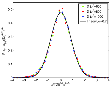
Figure 5: Collapse-plot for the tagged particle probability density function at different times. The solid black curve is a zero-mean Gaussian with a width given by Eq. (11). The symbols correspond to heterogeneity-averaged simulations over 8000 noise realizations with $N=501$ particles in a system of length L=5001b ($b$ is the particle size) with $\alpha=0.7$.

Appendix E Tracer particle dynamics in the presence of a time-varying external force.

To test the effective medium harmonization approach further we have considered the response of a tagged particle to an external force. For this purpose let us assume that a harmonically oscillating force $f_{n}(t)=\delta_{n,0}F_{0}\cos(\omega_{0}t)$ acts on particle $0$, where $\omega_{0}$ is the angular velocity and $F_{0}$ the force amplitude. From the formal solution Eq. (31) and Eq. (33) we find:

$$y(q,\omega)=\frac{\pi F_{0}[\delta(\omega-\omega_{0})+\delta(\omega+\omega_{0})]}{\kappa q^{2}-i\omega\xi_{\rm eff}(\omega)}.$$ (53)

Further, by performing the inverse Fourier-transform with respect to $q$, and setting $n=0$, we get

$$\langle y_{0}(t)\rangle_{f}=\frac{F_{0}}{2\kappa}{\rm Re}\left(\frac{e^{i\omega_{0}t}}{[-i\omega_{0}\xi_{\rm eff}(\omega_{0})/\kappa]^{1/2}}\right),$$ (54)

where ${\rm Re}\{..\}$ denotes the real part and the subscript indicates an average in the presence of a force. For a LT [HT] system we use the friction constant in Eq. (27) [Eq. (29)] in the expression above. Switching to the real tagged particle coordinate $x_{\mathcal{T}}$ assuming $\langle x_{\mathcal{T}}(t=0)\rangle=0$ we get $\langle x_{\mathcal{T}}(t)\rangle_{f}=[F_{0}/(2\sqrt{\kappa\bar{\xi}\omega_{0}})]\cos(\omega_{0}t-\phi)$ where $\phi=\pi/4$ for LT systems. For HT systems we find

$$\langle\delta x_{\mathcal{T}}(t)\rangle_{f}=\frac{F_{0}}{2\sqrt{\kappa\chi}\omega_{0}^{\delta}}\cos(\omega_{0}t-\phi)$$ (55)

with the non-trivial phase-shift $\phi=\delta\pi/2<\pi/4$.

Appendix F Generalized Einstein relation.

Suppose a static force $F_{0}$ is applied to particle $0$ at time $t=0$, i.e. $f_{n}(t)=F_{0}\delta_{n,0}\theta(t)$. From the fluctuation-dissipation theorem kubo66 , we have that the following simple relation holds between the tagged particle mean square displacement in the absence of the force $\langle\delta x_{\mathcal{T}}^{2}(t)\rangle$, and the mean displacement in the presence of the force $\langle\delta x_{\mathcal{T}}(t)\rangle_{F}$

$$\langle\delta x_{\mathcal{T}}(t)\rangle_{f}=\frac{F_{0}}{2k_{B}T}\langle\delta x_{\mathcal{T}}^{2}(t)\rangle$$ (56)

which is referred to as the generalized Einstein relation. A consistency check of the effective medium-harmonization formalism is thus to check that this relation holds. From Eq. (31) we straightforwardly compute the average velocity (in frequency space): $\langle v_{n}(\omega)\rangle=-i\omega\langle y_{n}(\omega)\rangle$ for the type of force considered here. Further, by Fourier-inverting and setting $n=\mathcal{T}=0$, and using Eq. (29) we find

$$\langle v_{\mathcal{T}}(t)\rangle=\frac{F_{0}}{2\sqrt{\kappa\chi}}\frac{t^{\delta-1}}{\Gamma(\delta)}\theta(t)$$ (57)

for HT systems. By integrating the expression above over time and comparing with the MSD in the main text we find that Eq. (56) is satisfied for $t>0$. A similar calculation for LT systems shows that indeed the generalized Einstein relation is satisfied also then.

Appendix G Simulation scheme

We consider $N$ hardcore particles of linear size $b$ in a box of length $L$ (the box extends from $-L/2$ to $L/2$). At random times the particles performs hops with the jump length taken from a Gaussian distribution of width $a$. Particle $n$ ($n=1,...,N$) has a hop rate $q_{n}$, where $q_{n}$ is related to the friction constant $\xi_{n}$ by $q_{n}=2k_{B}T/(\xi_{n}a^{2})$. We are interested in the stochastic dynamics of the center positions $X_{n}$ of all particles, when we have the single-file constraint $X_{n+1}-X_{n}>b$ at all times. Also, particles cannot move out of the box: $X_{1}>-(L-b)/2$ and $X_{N}<(L-b)/2$. Our numerical approach detailed below, builds on a previous scheme for lattice simulations called the trial-and-error Gillespie algorithm TA_etal . Our continuum version of that algorithm is:

1. Generate the cumulative sums of the free total rate constants

   $$p_{0} = 0,$$

   $$p_{n} = \sum_{m=1}^{n}q_{m},\qquad n=1,...,N.$$ (58)

2. Generate a random initial configuration of particle positions $X_{n}(0)$ ($n=1,...,N$). This step requires some care, see next section.

3. Set the time equal to zero, $t=0$.

4. Draw a uniform random number $r$ ($0<r<1$). Construct a waiting time $\tau$ according to:

   $$\tau=\frac{1}{p_{N}}\log\left(\frac{1}{r}\right),$$ (59)

   i.e. $\tau$ is taken from an exponential distribution $\Phi(\tau)\propto\exp(-\tau\sum_{n=1}^{N}q_{n})$. Update the time $t\rightarrow t+\tau$.

5. Draw a new uniform random number $r$ ($0<r<1$). A trial particle $n$ is determined by the $n$ which satisfies

   $$p_{n-1}\leq rp_{N}<p_{n}$$ (60)

   i.e., particle $n$ is chosen with a probability $\propto q_{n}$.

6. Draw a random attempt jump length $l$ from the Gaussian distribution of width $a$: $P(l)=(2\pi a^{2})^{-1/2}\exp[-(l-\mu)^{2}/(2a^{2})]$. For the case of a harmonically oscillating external force on the tracer particle $f_{n}(t)=\delta_{n,0}F_{0}\cos(\omega_{0}t)$, $\mu=\alpha_{0}\cos[\omega_{0}t])$ for the tracer particle with $\alpha_{0}=F_{0}/(\xi_{0}q_{0})$, otherwise $\mu=0$.

7. Loop over the neighboring particles in the direction of the attempted jump, and find the number $M$ of particles which have their center positions within a distance $l-b$ of their previous neighbor.

8. Draw a uniform random number $r$ and move particle $n$ and the $M$ neighbor particles a distance $l$ if $r<\xi_{n}/\sum_{m=n}^{n\pm M}\xi_{m}$ (the sum ranges from $n$ to $n+M$ if the attempted jump is to the right, otherwise the range is $n-M$ to $n$), and there is no wall preventing the move. If the move occurs then update the particle positions.

9. Return to step (4).

The scheme above produces a stochastic time series $X_{n}(t)$, and if steps (2)-(9) are repeated many times, ensemble averages can be computed. Note that step (1) does not have to be repeated for each simulation run (each realization of the noise) for the non-averaged case, i.e. if the free total hop rates are the same for all simulation runs. For the heterogeneity-averaged case, where we assign new hop rates for the particles for every new simulation run, step 1 has to be repeated for each one of them. An efficient method for performing the search for the $n$ satisfying the inequality in Eq. (60) was presented previously TA_etal . We here point out that in our previous study TA_etal we instead of Eq. (60) used $p_{n-1}<rp_{N}\leq p_{n}$. This criterion for choosing a trial particle causes the algorithm to get stuck for the (exceptional) case that $p_{n-1}\equiv rp_{N}$ if combined with the search algorithm in appendix B of Ref. TA_etal, . We are grateful to Karl Fogelmark for pointing this out to us.

In step 2 in our algorithm, we set the initial positions randomly (with the possible additional constraint of a fixed position for a tracer particle). For point-particles this present no problem - for completely random initial positioning one simply needs to draw $N$ uniform random numbers between $-L/2$ and $L/2$, which are then sorted and assigned as initial positions. For finite size particles one must make sure that there is no overlap of the particles. The same procedure as used above, with the additional step to discard configurations where two or more particle overlap, is very inefficient for large $N$. We instead use the following mapping between the finite-size particle problem [initial positions $X_{n}(0)$, $n=1,...,N$] and a point-particle problem [initial positions $\tilde{X}_{n}(0)$] LIAM1 ; LIAM2

$$L = l+Nb,$$

$$X_{n}(0) = \tilde{X}_{n}(0)+nb-\frac{N+1}{2}b.$$ (61)

Step 2 in the simulation scheme then becomes: draw random numbers between $-l/2$ and $l/2$ which, after sorting, gives $\tilde{X}_{n}(0)$. Then use the relation above to determine $X_{n}(0)$. This procedure is used in the simulations providing the dynamic structure factor. For the tracer particle simulations we fix the initial position of a tracer particle at the center of the system with equally many particles to the left and right. The procedure above then has to be done separately for the particles to the left and right of the tracer particle.

Step 7 and 8 constitute our rule for handling collisions between particles. These rules are based on the idea of having momentum conservation on average in collisions while at the same time fulfilling detailed balance. The total momentum dissipated to the surrounding medium if particle $n$ moves a distance $l$ is $l\xi_{n}$. When the $M+1$ particles move the dissipated momentum is $l\sum_{m=n}^{n\pm M}\xi_{m}$. Carrying out the later move with a probability $\xi_{n}/\sum_{m=n}^{n\pm M}\xi_{m}$ makes the dissipated momentum independent, on average, of whether collisions happen or not. Detailed balance is satisfied, because the rate for the attempted move of the $M+1$ particles is $q_{n}\propto 1/\xi_{n}$. Thus the rate at which the particles actually move will be proportional to $1/\xi_{n}\times\xi_{n}/\sum_{m=n}^{n\pm M}\xi_{m}=1/\sum_{m=n}^{n\pm M}\xi_{m}$, and identical to the rate with which the reverse move (particle $n\pm M$ initiating the reverse move of the $M+1$ particles in the opposite direction) occurs, since in equilibrium all allowed positions of the hard-core interacting particles are equally probable. Detailed balance is therefore satisfied by the above algorithm.

In the simulations of HT systems we draw the friction constants $\xi_{n}$ from the density [$0<\alpha<1$]

$$\varrho(\xi_{n})=A\xi_{n}^{-1-\alpha}\ {\rm for}\ \xi\geq\xi_{c}$$ (62)

and $\varrho(\xi_{n})=0$ for $\xi_{n}<\xi_{c}$. The normalization constant is $A=\alpha\xi_{c}^{\alpha}$. In order to generate a random friction constant $\xi_{n}$ according to the density above, in a standard fashion gillespie76 , we set the cumulative distribution $C(\xi_{n})=\int_{0}^{\xi_{n}}\varrho(\xi^{\prime})d\xi^{\prime}$ equal to a uniform random number $r$ between 0 and 1, $C(\xi_{n})=r$. Explicitly we then get

$$\xi_{n}=\xi_{c}(1-r)^{-1/\alpha}.$$ (63)

In each simulation we determine a random friction constant $\xi_{n}$ for each particle using Eq. (63). Then, using the fact that the free particle diffusion constant $D_{n}$ is related to the friction and hop rates as $D_{n}=q_{n}a^{2}/2=k_{B}T/\xi_{n}$, we get random hop rates: $q_{n}=2k_{B}T/(\xi_{n}a^{2})$ used in the simulations. We fix the normalization constant $A$ by setting the average diffusion constant $\bar{D}=k_{B}T\int\xi_{n}^{-1}\varrho(\xi_{n})d\xi_{n}=\alpha k_{B}T/[(1+\alpha)\xi_{c}]$ to unity in the simulations.

In all simulations except those for the structure factor $S(Q,t)$ we have used a width $a=1$ for the jump length distribution. For the structure factor simulations $a=0.25$ was used due to a higher choice of density $\rho$. Ideally $a$ should be as small as possible compared with the average distance between particles $\rho^{-1}$ to approximate the diffusive limit of moving particles in a spatial continuum.

References

- (1) K. Pearson. Nature, 72(1865):294, 1905.
- (2) L. Rayleigh. Nature, 72(1866):318, 1905.
- (3) M.E. Fisher. Journal of Statistical Physics, 34(5):667–729, 1984.
- (4) V. Kukla, J. Kornatowski, D. Demuth, I. Girnus, H. Pfeifer, L.V.C. Rees, S. Schunk, K.K. Unger, and J. Kärger. Science, 272(5262):702, 1996.
- (5) T. Meersmann, J.W. Logan, R. Simonutti, S. Caldarelli, A. Comotti, P. Sozzani, L.G. Kaiser, and A. Pines. J. Phys. Chem. A, 104(50):11665–11670, 2000.
- (6) K. Hahn, J. Kärger, and V. Kukla. Physical Review Letters, 76(15):2762–2765, 1996.
- (7) Q.H. Wei, C. Bechinger, and P. Leiderer. Science, 287(5453):625, 2000.
- (8) V. Gupta, S.S. Nivarthi, A.V. McCormick, and H. Ted Davis. Chemical Physics Letters, 247(4-6):596–600, 1995.
- (9) AL Hodgkin and RD Keynes. The Journal of Physiology, 128(1):28, 1955.
- (10) G.W. Li, O.G. Berg, and J. Elf. Nature Physics, 5(4):294–297, 2009.
- (11) D.G. Levitt. Physical Review A, 8(6):3050–3054, 1973.
- (12) R. Arratia. The Annals of Probability, 11(2):362–373, 1983.
- (13) T.E. Harris. Journal of Applied Probability, 2(2):323–338, 1965.
- (14) S. Alexander and P. Pincus. Physical Review B, 18(4):2011–2012, 1978.
- (15) M. Kollmann. Physical Review Letters, 90(18):180602, 2003.
- (16) E. Barkai and R. Silbey. Physical Review Letters, 102(5):50602, 2009.
- (17) L. Lizana and T. Ambjörnsson. Physical Review E, 80:051103, 2008.
- (18) L. Lizana, T. Ambjörnsson, A. Taloni, E. Barkai, and M.A. Lomholt. Physical Review E, 81:051118, 2010.
- (19) A.Y. Grosberg and A.R. Khokhlov. Statistical Physics of Macromolecules, AIP Press, New York, 1994.
- (20) R. Landauer. Journal of Applied Physics, 23:779, 1952.
- (21) S. Kirkpatrick. Physical Review Letters, 27(25):1722–1725, 1971.
- (22) S. Alexander, J. Bernasconi, WR Schneider, and R. Orbach. Reviews of Modern Physics, 53(2):175–198, 1981.
- (23) P. Gonçalves and M. Jara. Journal of Statistical Physics, 132(6):1135–1143, 2008.
- (24) O. Flomenbom, Phys. Rev. E 82, 031126 (2010).
- (25) T. Ambjörnsson, L. Lizana, M.A. Lomholt, and R.J. Silbey. The Journal of Chemical Physics, 129:185106, 2008.
- (26) M. Jara. E-print: arXiv:0901.0229, 2009.
- (27) R. Kubo. Rep. Prog. Phys., 29:255, 1966.
- (28) B.J. Berne and R. Pecora. Dynamic Light Scattering with applications to chemistry, biology and physics, Dover Pubns, 2000.
- (29) R. Metzler and J. Klafter. Physics Reports, 339(1):1–77, 2000.
- (30) L. Onsager. Phys. Rev., 37:405, 1931.
- (31) J. Szymanski and M. Weiss. Physical Review Letters, 103(3):38102, 2009.
- (32) S. Kirkpatrick. Percolation and Conduction, 45:574–588, 1973.
- (33) L. Lizana and T. Ambjörnsson. Physical Review Letters, 100(20):200601, 2008.
- (34) D.T. Gillespie. J. Comp. Phys., 22:403, 1976.