Dynamics of bubbles in a two-component Bose-Einstein condensate

Abstract

The dynamics of a phase-separated two-component Bose-Einstein condensate are investigated, in which a bubble of one component moves through the other component. Numerical simulations of the Gross–Pitaevskii equation reveal a variety of dynamics associated with the creation of quantized vortices. In two dimensions, a circular bubble deforms into an ellipse and splits into fragments with vortices, which undergo the Magnus effect. The Bénard–von Kármán vortex street is also generated. In three dimensions, a spherical bubble deforms into toruses with vortex rings. When two rings are formed, they exhibit leapfrogging dynamics.

I Introduction

A droplet of ink falling into water deforms from a sphere to a toroidal shape due to the formation of a vortex ring Thomson ; Yajima . An air bubble rising in water exhibits complicated dynamics such as zigzag and spiral motion Haberman ; Saffman . Such phenomena are caused by the interaction between the droplet (ink) or the bubble (air) with the medium (water), where the former moves through the latter. The subject of the present paper is the dynamics of phase-separated two-component superfluids in similar situations, that is, a bubble of one component moving through the other component.

A variety of dynamical properties have been observed in two-component Bose–Einstein condensates (BEC) Myatt . Two immiscible components prepared in a spatially overlapped state separate dynamically Hall and develop into a domain structure Miesner . A similar structure is observed in a miscible system with counterflow Hoefer . In rotating two-component BECs, a square vortex lattice has been observed Schweik . These dynamical properties of two-component BECs have been studied theoretically Chui ; Kasamatsu1 ; Law ; Ishino ; Mueller ; Kasamatsu2 . Theoretical predictions have been made on various structures in two-component BECs; for example, Skyrmions Ruo , solitary wave complexes Berloff , and vortex bright solitons KJHLaw . Various interface instabilities known in classical fluid mechanics are predicted to emerge in two-component BECs with an interface, namely the Rayleigh–Taylor instability Sasaki ; Gautam , the Kelvin–Helmholtz instability Takeuchi ; Suzuki , and the Richtmyer–Meshkov instability Bezett . The behavior of two-component BECs strongly depends on the miscibility, which is determined by the intra- and inter-component interactions. Recently, these interactions in two-component systems have been controlled using the Feshbach resonance Thal , and phase separation dynamics have been studied in a controlled manner Papp ; Tojo .

In the present paper, we investigate the dynamics of a bubble in a phase-separated two-component BEC, where a small fraction of one component moves through the other component. We show that the system exhibits a rich variety of dynamics depending on the parameters and dimensionality. In two dimensions (2D), a circular bubble at rest deforms into an ellipse as it accelerates and breaks into pieces with quantized vortices. For strong phase separation, a vortex street is formed in the wake of the moving bubble, as in the Bénard–von Kármán vortex street in a single-component BEC SasakiL . In three dimensions (3D), a spherical bubble deforms into a torus, as in classical fluids Thomson ; Yajima . The significant difference from classical fluids is that the toroidal bubble is accompanied by a quantized vortex ring. When two or more rings are generated, they leapfrog each other.

This paper is organized as follows. Section II provides a formulation of the problem. Section III.1 numerically demonstrates the dynamics of a 2D system and Sec. III.2 analyzes the deformation of a bubble. Section IV performs full 3D numerical simulations. Section V gives conclusions to this study.

II Formulation of the problem

We study the dynamics of a two-component BEC using the zero-temperature mean-field theory. The dynamics of the system are described by the Gross–Pitaevskii (GP) equation given by

$$i\hbar\frac{\partial\psi_{1}}{\partial t} = \left(-\frac{\hbar^{2}}{2m_{1}}\nabla^{2}+V_{1}\right)\psi_{1}+g_{11}|\psi_{1}|^{2}\psi_{1}$$ (1a)

$$+g_{12}|\psi_{2}|^{2}\psi_{1},$$

$$i\hbar\frac{\partial\psi_{2}}{\partial t} = \left(-\frac{\hbar^{2}}{2m_{2}}\nabla^{2}+V_{2}\right)\psi_{2}+g_{22}|\psi_{2}|^{2}\psi_{2}$$ (1b)

$$+g_{12}|\psi_{1}|^{2}\psi_{2},$$

where $\psi_{j}$ is the macroscopic wave function, $m_{j}$ is the atomic mass, and $V_{j}$ is the external potential for the $j$th component ($j=1,2$). The interaction parameters $g_{jj^{\prime}}$ are defined as

$$g_{jj^{\prime}}=2\pi\hbar^{2}a_{jj^{\prime}}(m_{j}^{-1}+m_{j^{\prime}}^{-1}),$$ (2)

where $a_{jj^{\prime}}$ is the $s$-wave scattering length between the atoms in the $j$th and $j^{\prime}$th components.

We assume that the interaction parameters satisfy

$$g_{11}g_{22}>g_{12}^{2},$$ (3)

and therefore the two components are phase separated Pethick . We also assume that the external potentials for both components are initially absent, $V_{1}=V_{2}=0$. We consider an initial state in which a small fraction of component 2 is localized and surrounded by component 1, and $\psi_{1}$ is uniform far from component 2. The ground state is therefore a circular (2D) or spherical (3D) “bubble” of component 2 located in the sea of component 1. At $t=0$, we start to exert a force $F$ on the bubble by applying a potential $V_{2}=Fx$ to component 2. The bubble then moves in the $-x$ direction. This is done, e.g., by applying a magnetic field gradient to a system in which the atoms in component 2 have a magnetic dipole moment in the direction of the magnetic field while those in component 1 do not.

We numerically solve Eq. (1) by the pseudo-spectral method. The initial state is the ground state for $V_{1}=V_{2}=0$ obtained by the imaginary-time propagation method. We add a small amount of white noise to the initial state to break the numerically exact symmetry. The boundary in the numerical calculation is set far from the relevant region so that the periodic boundary condition does not affect the results. In the following analysis, we assume $m_{1}=m_{2}\equiv m$ and $g_{11}=g_{22}\equiv g$ to reduce the number of parameters.

III Two-dimensional system

III.1 Dynamics

We first demonstrate the numerical results for the 2D system. The wave function is assumed to have the form $\psi_{j}(\bm{r},t)=\psi_{j\perp}(x,y,t)\phi(z)$, where the dynamics of the normalized wave function $\phi(z)$ are frozen. Integrating the GP equation with respect to $z$, the effective interaction strength is found to be $g_{jj^{\prime}}\int|\phi|^{4}dz$. Hence, the healing length is $\xi_{\rm 2D}=\hbar/(mgn_{\rm 2D}\int|\phi|^{4}dz)^{1/2}$ and the sound velocity is $v_{\rm s}^{\rm 2D}=(gn_{\rm 2D}\int|\phi|^{4}dz/m)^{1/2}$, where $n_{\rm 2D}$ is the 2D density $|\psi_{1\perp}|^{2}$ far from the bubbles. Normalizing length and time by $\xi_{\rm 2D}$ and $\xi_{\rm 2D}/v_{\rm s}^{\rm 2D}$, the intra-component interaction parameter in the GP equation becomes unity and the relevant interaction parameter is only $g_{12}/g$.

Figure 1: (Color online) Time evolution of the normalized density distribution $\tilde{n}_{j}=|\psi_{j\perp}|^{2}/n_{\rm 2D}$ for $g_{12}/g=1.25$. From $\tilde{t}=tv_{\rm s}^{\rm 2D}/\xi_{\rm 2D}=0$ to $\tilde{t}=200$, the force $\tilde{F}=F\xi_{\rm 2D}^{2}/(\hbar v_{\rm s}^{\rm 2D})=1.58\times 10^{-3}$ is exerted on component 2 in the $-x$ direction. The amount of component 2 is $\int|\psi_{2}|^{2}dxdy/(n_{\rm 2D}\xi_{\rm 2D}^{2})=205$. The field of view is $158\times 126$ in units of $\xi_{\rm 2D}$.

Figure 1 shows the time evolution of the density distribution. The initial state is a circular bubble as shown in Fig. 1 (a). At $t=0$, we apply a potential $V_{2}=Fx$ to component 2, and the bubble is accelerated in the $-x$ direction. We find that the bubble is deformed in an elliptic shape as shown in Fig. 1 (b). After the potential $V_{2}$ is switched off at $\tilde{t}=tv_{\rm s}^{\rm 2D}/\xi_{\rm 2D}=200$, the bubble moves at a constant velocity keeping the elliptic shape as shown in Fig. 1 (c). Such elliptic deformation of a bubble is known in classical fluid mechanics Haberman and will be analyzed in Sec. III.2.

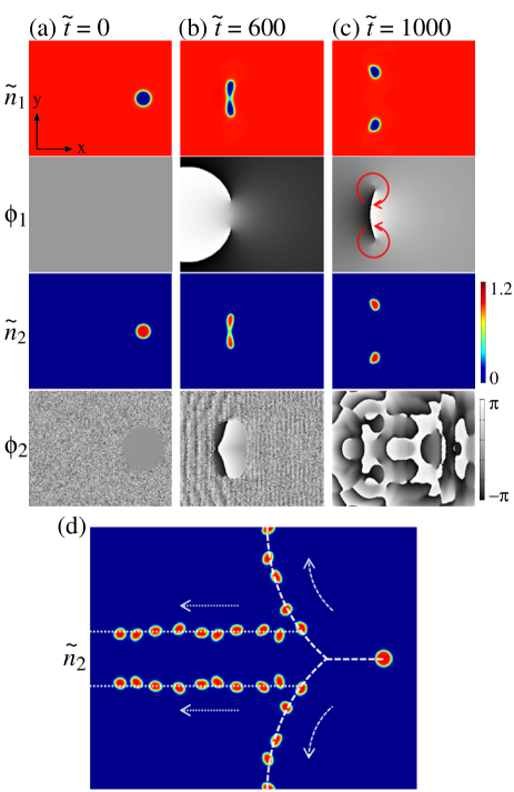
Figure 2: (Color online) (a)-(c) Time evolution of the density $\tilde{n}_{j}$ and phase $\phi_{j}={\rm arg}\psi_{j}$ profiles. The force $\tilde{F}=1.58\times 10^{-3}$ is kept constant for $t>0$. Other parameters are the same as those in Fig. 1. The arrows indicate the directions of circulation of the vortices. (d) Stroboscopic trajectories of component 2, where the images are taken at an interval of $\delta\tilde{t}=1000$. The force is constant for the images lying on the dashed lines, and the force is switched off at $\tilde{t}=1000$ for the images lying on the dotted lines. The field of view is $158\times 126$ in (a)-(c) and $316\times 253$ in (d) in units of $\xi_{\rm 2D}$.

Figures 2 (a)-2 (c) show the dynamics for the same parameters as those in Fig. 1, where the force is exerted for $t>0$. The bubble is first deformed elliptically as in Fig. 1 (b) and then splits into two bubbles [Figs. 2 (b) and 2 (c)]. We note that component 1 contains singly-quantized vortices with opposite circulations at the split bubbles as indicated by the arrows in Fig. 2 (c). After the split, the two bubbles move away from each other as shown by the dashed lines in Fig. 2 (d), and eventually move in the directions perpendicular to the force. This behavior is due to the Magnus force on the vortices given by

$$\bm{F}_{\rm M}=\rho\bm{\kappa}\times\bm{v},$$ (4)

where $\rho$ is the mass density, $\bm{\kappa}$ is the vorticity, and $\bm{v}$ is the velocity of the vortex. In this case, $\rho\simeq mn_{\rm 2D}$ and $\kappa=2\pi\hbar/m$. The velocity of the bubbles in the $\pm y$ directions is estimated by equating the Magnus force in the $+x$ direction and the external force on the bubble in the $-x$ direction as

$$mn_{\rm 2D}\frac{2\pi\hbar}{m}v_{y}=F\int|\psi_{2\perp}|^{2}dxdy,$$ (5)

where the integration is taken within one of the bubbles. For the parameters in Fig. 2, the velocity is estimated from Eq. (5) to be $v_{y}/v_{\rm s}^{2D}\simeq 0.026$, which is in good agreement with the velocity $\simeq 0.026$ along the dashed line in Fig. 2 (d). If the external potential for component 2 is switched off after the bubble splits, the two bubbles move in the $-x$ direction at a constant velocity $\simeq\kappa/(2\pi d)$ with a constant distance $d$ maintained between the bubbles, as shown by the dotted lines in Fig. 2 (d). Such a two-component vortex is suitable for studying the Magnus effect, since we can exert a force on the vortex in a controlled manner.

Figure 3: (Color online) (a)-(f) Time evolution of the density profile of component 1, where the force $\tilde{F}=4.74\times 10^{-3}$ is exerted on component 2 from $\tilde{t}=0$ to $\tilde{t}=500$. The other conditions are the same as those in Fig. 1. The two vortex pairs are marked by black and white circles to follow their motion. (g) Phase profile of component 1 at $\tilde{t}=500$. The field of view in (a)-(g) is $316\times 126$ in units of $\xi_{\rm 2D}$.

Figures 3 (a)-3 (f) shows the time evolution of the density profile of component 1, where the force is stronger than that in Figs. 1 and 2. At $\tilde{t}=300$, the bubble releases two fragments, at which point component 1 has a vortex-antivortex pair [two white circles in Fig. 3 (a)]. The preceding bubble then splits into two, at which point a vortex-antivortex pair is also contained in component 1 [black circles in Fig. 3 (b)]. After that, the pair marked by the white circles passes through that marked by the black circles, and the two pairs leapfrog each other back and forth as shown in Figs. 3 (c)-3 (f).

Figure 4: (Color online) Snapshots of the density and phase profiles for $g_{12}/g=3.3$. The force on component 2 is $\tilde{F}=6.96\times 10^{-3}$ in (a) and $\tilde{F}=6.01\times 10^{-3}$ in (b). The black crosses in (a) indicate the positions of the bubble at an interval of $\Delta\tilde{t}=200$. The field of view is $-869\xi_{\rm 2D}<x<-474\xi_{\rm 2D}$ and $-158\xi_{\rm 2D}<y<158\xi_{\rm 2D}$ in (a) and $-869\xi_{\rm 2D}<x<-474\xi_{\rm 2D}$ and $-63\xi_{\rm 2D}<y<63\xi_{\rm 2D}$ in (b), where the initial spherical bubble is located at $x=y=0$. The amount of component 2 is the same as that in Fig. 1.

Figure 4 shows the cases for strong force and strong phase separation. Since the interface tension is large for strong phase separation Barankov ; Schae , the bubble is hard to split as in Fig. 2. Consequently, the bubble is accelerated beyond the critical velocity for vortex creation and the vortices are shed in the wake as shown in Fig. 4. Figure 4 (a) shows a typical behavior of the bubble, in which the Magnus force bends the trajectory of the bubble while it contains vortices and then the bubble moves in a winding fashion since the vorticity contained in the bubble changes in time. Occasionally, vortices are shed in pairs periodically as shown in Fig. 4 (b), which is reminiscent of the Bénard–von Kármán vortex street in a single-component BEC SasakiL . Unlike vortex shedding in a single-component BEC, the bubble gradually diminishes because the cores of the released vortices are occupied by component 2 as shown in the bottom panel of Fig. 4 (b). The condition thus continuously changes and the vortex street generation does not last long, since the parameter region for the vortex street generation is narrow SasakiL .

III.2 Analysis of bubble deformation

To understand the elliptic deformation of the 2D bubble shown in Fig. 1, we perform a simple analysis.

In this subsection, we assume that the thickness of the interface between the two components is negligible due to the strong phase separation, and the effect of the interface is expressed only by an interface tension coefficient $\alpha$. The wave function of the stationary state of component 1 outside the bubble is written as $\psi_{1}(\bm{r},t)=n_{1}^{1/2}(\bm{r})\exp[i\theta_{1}(\bm{r})-i\mu_{1}t/\hbar]$, where we consider the problem in the frame moving with the bubble. Substituting this expression into the GP equation (1), we obtain

$$\nabla\cdot[n_{1}(\bm{r})\bm{v}_{1}(\bm{r})] = 0,$$ (6)

$$-\frac{\hbar^{2}}{2m}\frac{\nabla^{2}\sqrt{n_{1}(\bm{r})}}{\sqrt{n_{1}(\bm{r})}}+\frac{1}{2}mv_{1}^{2}(\bm{r})+g_{11}n_{1}(\bm{r}) = \mu_{1},$$ (7)

where $\bm{v}_{1}=\hbar\nabla\theta_{1}/m$. We also assume that the system is almost incompressible, i.e., $n_{j}(\bm{r})=\bar{n}_{j}+\delta n_{j}(\bm{r})$ with $\delta n_{j}(\bm{r})\ll\bar{n_{j}}$. Equations (6) and (7) then become

$$\nabla\cdot\bm{v_{1}}(\bm{r}) \simeq 0,$$ (8)

$$P_{1}(\bm{r})+\frac{1}{2}\bar{n}_{1}mv_{1}^{2}(\bm{r}) \simeq {\rm const.},$$ (9)

where $P_{1}(\bm{r})=g_{11}n_{1}^{2}(\bm{r})/2$ is the pressure. Equation (9) corresponds to Bernoulli’s equation in classical fluid mechanics.

The shape of the bubble is approximated to be an ellipse given by $x^{2}/a^{2}+y^{2}/b^{2}=1$, and we estimate $a$ and $b$ considering the pressure inside and outside the bubble at $\bm{r}_{a}=(a,0)$ and $\bm{r}_{b}=(b,0)$. Since $v_{1}=0$ at the stagnation point $\bm{r}_{a}$, Eq. (9) gives

$$P_{1}(\bm{r}_{a})=P_{1}(\bm{r}_{b})+\frac{1}{2}\bar{n}_{1}mv_{1}^{2}(\bm{r}_{b}).$$ (10)

For inviscid and incompressible flow, the velocity on either side of an elliptic obstacle is $v_{1}(\bm{r}_{b})=v_{0}(a+b)/a$ Lamb , where $v_{0}$ is the velocity at infinity. Applying Laplace’s formula Landau to the inner pressure at $\bm{r}_{a}$ and $\bm{r}_{b}$, we have

$$P_{1}(\bm{r}_{a})+\alpha\frac{a}{b^{2}}=P_{1}(\bm{r}_{b})+\alpha\frac{b}{a^{2}},$$ (11)

where $a/b^{2}$ and $b/a^{2}$ are the curvatures of an ellipse at $\bm{r}_{a}$ and $\bm{r}_{b}$, respectively. Using Eqs. (10) and (11), we obtain an expression that estimates the oblateness of the bubble as

$$\frac{m\bar{n}_{1}v_{0}^{2}}{2\alpha}\sqrt{\frac{A}{\pi}}=\sqrt{\beta}\frac{1-\beta^{3}}{(1+\beta)^{2}},$$ (12)

where $A=\pi ab$ is the area of the ellipse and $\beta=a/b$. The left-hand side of Eq. (12) corresponds to the Weber number in fluid mechanics.

Figure 5: (Color online) Oblateness $\beta$ of an elliptic bubble as a function of the velocity $v_{0}$. The solid curve shows Eq. (12) with the interface tension coefficient $\alpha$ in Eq. (13). The dotted curve shows Eq. (12) with the left-hand side multiplied by 1.2. The circles are numerically obtained from the GP equation. The inset shows an example of the density distribution of component 2 for a stationary state.

We compare Eq. (12) with the numerical calculation. We numerically solve Eq. (1) with $V_{1}=V_{2}=0$ and $-iv_{0}\partial_{x}\psi_{j}$ added to the right-hand side. The imaginary time propagation of this equation gives the stationary state in the frame moving in the $-x$ direction with velocity $v_{0}$. The circles in Fig. 5 plot the ratio of the size of the bubble in the minor axis to that in the major axis as a function of the velocity. The solid curve in Fig. 5 shows Eq. (12) with the interface tension coefficient Barankov ; Schae ,

$$\alpha=\frac{\hbar\bar{n}_{1}^{3/2}}{\sqrt{2m}}\sqrt{g_{12}-g}.$$ (13)

We find that the solid curve deviates from the circles. The deviation of the analytic result from the numerical result may be due to the approximations and assumptions made in the analysis. This deviation can be compensated if we modify Eq. (12). The dotted curve in Fig. 5 shows Eq. (12) with the left-hand side multiplied by 1.2, which is in good agreement with the circles in Fig. 5.

IV Three dimensional system

In the numerical simulations in 3D, we normalize length and time by $\xi=\hbar/(mgn_{\rm 3D})^{1/2}$ and $\xi/v_{\rm s}$, where $n_{\rm 3D}$ is the atom density far from the bubbles and $v_{\rm s}=(gn_{\rm 3D}/m)^{1/2}$ is the sound velocity.

Figure 6: (Color online) (a)-(d) Time evolution of the isodensity surface of component 2 in the 3D simulation. The size of the frame is $178\times 63\times 63$ in units of $\xi$. (e) Density $\tilde{n}_{1}=|\psi_{1}|^{2}/n_{\rm 3D}$ and phase $\phi_{1}={\rm arg}\psi_{1}$ profiles of component 1 on the $z=0$ cross section at $\tilde{t}=tv_{\rm s}/\xi=560$. The field of view is $178\times 63$ in units of $\xi$. The parameters are $g_{12}/g=1.1$, $\tilde{F}=F\xi^{2}/(\hbar v_{\rm s})=3.2\times 10^{-3}$, and $\int|\psi_{2}|^{2}d\bm{r}/(n_{\rm 3D}\xi^{3})=3.2\times 10^{3}$.

Figures 6 (a)-6 (d) show typical dynamics of a bubble in 3D. The initial state is a spherical bubble [Fig. 6 (a)], which deforms into a ellipsoidal shape as it is accelerated [Fig. 6 (b)]. The bubble then takes a toroidal shape [Fig. 6 (c)], whose radius increases in time [Fig. 6 (d)]. Since the amount of component 2, $\int|\psi_{2}|^{2}d\bm{r}$, is conserved, the torus becomes thin as its radius increases. Figure 6 (e) shows the density and phase profiles on the cross section of $z=0$ at $\tilde{t}=tv_{\rm s}/\xi=560$. We find that component 1 contains a quantized vortex ring along the torus of component 2. If the force on component 2 is switched off after the ring is formed, the ring propagates in the $-x$ direction at a constant velocity without expansion of the radius. The velocity roughly agrees with $v\simeq\hbar/(2mR)\ln(8R/a)$ Fetter , where $R$ is the radius of the torus and $a$ is the radius of the vortex core.

In contrast to a vortex ring in a single component superfluid Rayfield , we can manipulate the vortex ring by applying a potential to the torus of component 2 using a magnetic field gradient or laser field. We also note that a Skyrmion Ruo can be created if we imprint the phase ${\rm arg}(z\pm iy)$ on the torus of component 2 using, e.g., the Raman transition with Laguerre–Gaussian beams Andersen .

Figure 7: (Color online) Time evolution of the isodensity surface of component 2 in the 3D simulation. The force is $\tilde{F}=9.5\times 10^{-3}$ and the other parameters are the same as those in Fig. 6. The two objects are color coded for clarity. The size of the frame is $221\times 63\times 63$ in units of $\xi$.

When the force $F$ is strong, we can create multiple rings as shown in Fig. 7, where the two rings are color coded to distinguish them. The initial state is the same as that in Fig. 6 (a). The bubble first releases a ring backwards [Fig. 7 (a)] and then the front bubble also deforms into a ring [Fig. 7 (b)], resulting in double vortex rings with the same circulation. After that, the rear ring passes through the front ring [Figs. 7 (c) and 7 (d)], and this overtaking is repeated [Figs. 7 (d) and 7 (f)], which is the 3D version of the behavior in Fig. 3. Such a leapfrogging behavior of vortex rings was first predicted in Ref. Helmholtz .

V Conclusions

We have investigated the dynamics of phase-separated two-component BECs, in which a “bubble” of one component propagates in the other component. We studied 2D systems in Sec. III. When the velocity of the bubble is small, the circular bubble deforms into an elliptic shape, which travels with a constant velocity if the force is switched off (Fig. 1). The elliptic deformation of the bubble was analyzed in Sec. III.2. For a large velocity, the bubble of component 2 splits into two or more fragments, where component 1 contains quantized vortices (Figs. 2 and 3). The trajectories of bubbles containing vortices are then affected by the Magnus force [Fig. 2 (d)]. When the force and phase separation are strong, vortex shedding occurs instead of the split. The bubble drifts due to the Magnus force and sometimes generates the Bénard–von Kármán vortex street (Fig. 4). For the 3D system studied in Sec. IV, we found that the spherical bubble changes to a toroidal shape, where component 1 contains a quantized vortex ring (Fig. 6). When two vortex pairs or two vortex rings are created, they exhibit a leapfrog behavior (Figs. 3 and 7).

We have thus shown that bubbles in two-component BECs exhibit a rich variety of phenomena. When the bubble of component 2 splits in 2D or becomes a torus in 3D, quantized vortices are generated in component 1, whose cores are occupied by component 2. We can therefore exert a force on the vortices in component 1 in a controlled manner through the force on component 2, which may allow manipulation of vortices in a BEC.

- (1) J. J. Thomson and H. F. Newall, Proc. Roy. Soc. London 39, 417 (1885).
- (2) S. Yajima, Nature (London) 133, 414 (1934).
- (3) W. L. Haberman and R. K. Morton, David Taylor Model Basin Report No. 802 (1953).
- (4) P. G. Saffman, J. Fluid Mech. 1, 249 (1956).
- (5) C. J. Myatt, E. A. Burt, R. W. Ghrist, E. A. Cornell, and C. E. Wieman, Phys. Rev. Lett. 78, 586 (1997).
- (6) D. S. Hall, M. R. Matthews, J. R. Ensher, C. E. Wieman, and E. A. Cornell, Phys. Rev. Lett. 81, 1539 (1998).
- (7) H. -J. Miesner, D. M. Stamper-Kurn, J. Stenger, S. Inouye, A. P. Chikkatur, and W. Ketterle, Phys. Rev. Lett. 82, 2228 (1999).
- (8) M. A. Hoefer, C. Hamner, J. J. Chang, and P. Engels, arXiv:1007.4947.
- (9) V. Schweikhard, I. Coddington, P. Engels, S. Tung, and E. A. Cornell, Phys. Rev. Lett. 93, 210403 (2004).
- (10) S. T. Chui, H. Chui, H. Shi, W. M. Liu, W. -M. Zheng, Physica B (Amsterdam) 329, 36 (2003).
- (11) K. Kasamatsu and M. Tsubota, Phys. Rev. Lett. 93, 100402 (2004).
- (12) C. K. Law, C. M. Chan, P. T. Leung, and M.-C. Chu, Phys. Rev. A 63, 063612 (2001).
- (13) H. Takeuchi, S. Ishino, and M. Tsubota, Phys. Rev. Lett. 105, 205301 (2010).
- (14) E. J. Mueller and T. -L. Ho, Phys. Rev. Lett. 88, 180403 (2002).
- (15) K. Kasamatsu, M. Tsubota, and M. Ueda, Phys. Rev. Lett. 91, 150406 (2003).
- (16) J. Ruostekoski and J. R. Anglin, Phys. Rev. Lett. 86, 3934 (2001).
- (17) N. G. Berloff, Phys. Rev. Lett. 94, 120401 (2005).
- (18) K. J. H. Law, P. G. Kevrekidis, and L. S. Tuckerman, Phys. Rev. Lett. 105, 160405 (2010).
- (19) K. Sasaki, N. Suzuki, D. Akamatsu, and H. Saito, Phys. Rev. A 80, 063611 (2009).
- (20) S. Gautam and D. Angom, Phys. Rev. A 81, 053616 (2010).
- (21) H. Takeuchi, N. Suzuki, K. Kasamatsu, H. Saito, and M. Tsubota, Phys. Rev. B 81, 094517 (2010).
- (22) N. Suzuki, H. Takeuchi, K. Kasamatsu, M. Tsubota, and H. Saito, Phys. Rev. A (in press).
- (23) A. Bezett, V. Bychkov, E. Lundh, D. Kobyakov, and M. Marklund, Phys. Rev. A 82, 043608 (2010).
- (24) G. Thalhammer, G. Barontini, L. De Sarlo, J. Catani, F. Minardi, and M. Inguscio, Phys. Rev. Lett. 100, 210402 (2008).
- (25) S. B. Papp, J. M. Pino, and C. E. Wieman, Phys. Rev. Lett. 101, 040402 (2008).
- (26) S. Tojo, Y. Taguchi, Y. Masuyama, T. Hayashi, H. Saito, and T. Hirano, Phys. Rev. A 82, 033609 (2010).
- (27) K. Sasaki, N. Suzuki, and H. Saito, Phys. Rev. Lett. 104, 150404 (2010).
- (28) C. J. Pethick and H. Smith, Bose-Einstein Condensation in Dilute Gases, 2nd ed. (Cambridge University Press, Cambridge, 2008).
- (29) R. A. Barankov, Phys. Rev. A 66, 013612 (2002).
- (30) B. Van Schaeybroeck, Phys. Rev. A 78, 023624 (2008); 80, 065601 (2009).
- (31) See, for example, H. Lamb, Hydrodynamics, 6th ed (Dover, New York, 1945).
- (32) See, for example, L. D. Landau and E. M. Lifshitz, Fluid Mechanics, 2nd ed. (Butterworth-Heinemann, Oxford, 1987).
- (33) A. L. Fetter, Phys. Rev. 151, 100 (1966).
- (34) G. W. Rayfield and F. Reif, Phys. Rev. 136, A1194 (1964).
- (35) M. F. Andersen, C. Ryu, P. Cladé, V. Natarajan, A. Vaziri, K. Helmerson, and W. D. Phillips, Phys. Rev. Lett. 97, 170406 (2006).
- (36) H. von Helmholtz, Crelle’s J. 55, 25 (1858) [Phil. Mag. Ser. 4 33, 485 (1867)].