HIP-2010-32/TH

Spatial scalar correlator in strongly coupled hot ${\cal N}=4$ Yang-Mills theory

K. Kajantie^a,b, M. Vepsäläinen^a

^aDepartment of Physics, P.O.Box 64, FI-00014 University of Helsinki, Finland
^bHelsinki Institute of Physics, P.O.Box 64, FI-00014 University of Helsinki, Finland

We use AdS/CFT duality to compute in ${\cal N}=4$ Yang-Mills theory the finite temperature spatial correlator $G(r)$ of the scalar operator $F^{2}$, integrated over imaginary time. The computation is carried out both at zero frequency and integrating the spectral function over frequencies. The result is compared with a perturbative computation in finite $T$ SU($N_{c}$) Yang-Mills theory.

1 Introduction

A project to numerically study spatial correlators $G(r)$ of the scalar and pseudoscalar operators ${\rm Tr\,}F^{2}$ and ${\rm Tr\,}F\tilde{F}$ in finite temperature gauge field theory has been initiated in [1, 2]. Analytic computations of this correlator in next-to-leading order QCD perturbation theory have been carried out in [3, 4]. The purpose of this note is to compute this imaginary-time integrated entirely static correlator in supersymmetric ${\cal N}=4$ Yang-Mills theory using AdS/CFT duality. There is a standard framework for this [5, 6, 7, 8, 9], but the computation of full $r$ dependence involves some subtleties in the subtraction of divergences in the $\omega,k$ plane so that it is perhaps motivated to report on the details of the computation.

Concretely, we want to compute the finite $T$ correlator, of dimension 7,

$$G(r)=\int_{0}^{\beta}d\tau\,\langle F^{2}(\tau,{\bf x})F^{2}(0,{\bf 0})\rangle_{T}=\int_{0}^{\beta}d\tau\,G(\tau,{\bf x}),\quad F^{2}\equiv\textstyle{\frac{1}{4}\,}F_{\mu\nu}^{a}F_{\mu\nu}^{a},\quad r=|{\bf x}|.$$ (1)

This correlator is purely static, $\omega=0$, and we shall determine it by first evaluating its 3d Fourier transform $G(k)$, of dimension 4, and then transforming to coordinate space:

$$G(r)={1\over 2\pi^{2}r}\int_{0}^{\infty}dk\,k\sin(rk)G(k).$$ (2)

Hereby it is essential to separate the vacuum part from the finite $T$ part:

$$G(k)=G_{\mbox{\scriptsize vac}}(k)+[G(k)-G_{\mbox{\scriptsize vac}}(k)]=G_{\mbox{\scriptsize vac}}(k)+G_{T}(k).$$ (3)

We shall include in $G_{\mbox{\scriptsize vac}}(k)$ all constant terms and evaluate them analytically. Transforming to coordinate space they lead to contact terms proportional to $\delta({\bf x})$, but they have to be subtracted in numerics and their precise value is important. Furthermore, we show that at large $k$, $G_{T}(k)$ can be expanded in powers of $1/k^{4}$ and evaluate analytically the terms up to order $1/k^{8}$.

Although the main result can be obtained by taking $\omega=0$, it is also of interest to see with what happens when the real time frequency $\omega$ is included. Computing $G(\omega,{\bf k})$ and, in particular, the spectral function $\rho(\omega,{\bf k})\equiv{\rm Im\,}G_{R}(\omega,{\bf k})$ using the methods of [5, 6, 7, 8], the coordinate space Green’s function is given by

$$G(\tau,{\bf x})=\int{d^{3}k\over(2\pi)^{3}}e^{i{\bf x}\cdot{\bf k}}\int_{0}^{\infty}{d\omega\over\pi}\rho(\omega,{\bf k}){\cosh(\textstyle{\frac{1}{2}\,}\beta-\tau)\omega\over\sinh\textstyle{\frac{1}{2}\,}\beta\omega}.$$ (4)

Integrating this over $\tau$ we see that the static correlator is also obtained by evaluating

$$G(r)={1\over 2\pi^{2}r}\int_{0}^{\infty}dk\,k\sin(rk)\int_{0}^{\infty}{d\omega\over\pi}{2\rho(\omega,k)\over\omega}.$$ (5)

We shall show that the same result is obtained via (2) and (5), though the path via (5) is much longer. An essential part of the computation is again correct identification and elimination of divergences. Furthermore, interesting special nonstatic cases are the zero momentum temporal correlator $G(\tau,{\bf k}=0)$ and the equal time correlator $G(\tau=0,r)$. We shall comment on these at the end. An AdS/CFT computation of $G(\tau,r)$ has been presented in [2].

2 Equations

In the standard framework [5, 6, 7, 8] and notation, one takes the background

$$ds^{2} = b^{2}(z)\left(-f(z)dt^{2}+d{\bf x}^{2}+{dz^{2}\over f(z)}\right),$$ (6)

$$b(z) = {{\cal L}\over z},\quad f(z)=1-{z^{4}\over z_{h}^{4}},\quad{{\cal L}^{3}\over 4\pi G_{5}}={N_{c}^{2}\over 2\pi^{2}},$$ (7)

and the scalar field equation therein:

$$\ddot{\phi}+\biggl{(}{3\dot{b}\over b}+{\dot{f}\over f}\biggr{)}\dot{\phi}+\biggl{(}{\omega^{2}\over f^{2}}-{k^{2}\over f}\biggr{)}\phi=0,$$ (8)

where $\phi\equiv\phi(z,\omega,k)\equiv\phi(z,K)$, $k=|{\bf k}|$ . Scaling all dimensionful quantities with $z_{h}$ the equation becomes

$$\ddot{\phi}-{3+z^{4}\over z(1-z^{4})}\dot{\phi}+\biggl{[}{\omega^{2}\over(1-z^{4})^{2}}-{k^{2}\over 1-z^{4}}\biggr{]}\phi=0,$$ (9)

where

$$\omega\to z_{h}\omega={\omega\over\pi T},\quad k\to z_{h}k={k\over\pi T}.$$ (10)

Since

$$P(z)\equiv{3\dot{b}\over b}+{\dot{f}\over f}={d\over dz}\log(b^{3}f)$$ (11)

the Wronskian of two any linearly independent solutions of (8) is, integrating $\dot{W}/W=-P$,

$$W(\phi_{1},\phi_{2})=\phi_{1}\phi_{2}^{\prime}-\phi_{2}\phi_{1}^{\prime}={\bar{W}_{0}\over b^{3}f}=W_{0}{z^{3}\over 1-z^{4}},$$ (12)

where $W_{0}$ is a $z$ independent constant (but will depend on $\omega,k$).

2.1 The static case, $\omega=0$

As explained in the introduction, our goal is to compute the correlator in the static limit $\omega=0$. In this case it is a purely Euclidean quantity, and the equation to be solved is simply

$$\ddot{\phi}-{3+z^{4}\over z(1-z^{4})}\dot{\phi}-{k^{2}\over 1-z^{4}}\phi=0\,,$$ (13)

with the boundary conditions $\phi(0)=1$ and $|\phi(1)|<\infty$. While the full solution of this equation is very complicated, its behavior at large $k$ can be extracted. The leading term will give the vacuum part of the correlator, which diverges as $k^{4}$ and has to be subtracted before Fourier transforming our numerical results into coordinate space. The subleading terms will enable us to analytically compare the short-distance limit of our result with that in perturbative QCD [4], and also to have better control over the numerics.

To find the $k\to\infty$ limit of (13), the simplest method is to scale the variable as $y=kz$ and expand in $1/k^{4}$. The resulting differential equations are then solved order by order in $k^{-4}$, with the requirement that the solution stay finite at $z\approx 1$. The leading terms and their expansion at small $z$ are

$$\phi(z,k) =\textstyle{\frac{1}{2}\,}y^{2}K_{2}(y)+{1\over k^{4}}\cdot{1\over 20}\bigl{[}y^{6}K_{2}(y)-y^{7}K_{1}(y))\bigr{]}+{\cal O}(k^{-8})$$

$$\approx 1-\textstyle{\frac{1}{4}\,}(kz)^{2}-\textstyle{\frac{1}{16}\,}k^{4}z^{4}(\ln{\textstyle{1\over 2}}k+\ln z+\gamma_{E}-\textstyle{\frac{3}{4}\,})+\textstyle{\frac{1}{10}\,}z^{4}+{\cal O}(z^{6}).$$ (14)

The constant term $1/10$ will be important in numerics.

This method, while intuitive, is hard to implement beyond this point, as each new order requires solving an inhomogeneous differential equation on the whole interval $0\leq y<\infty$ to keep track of the boundary conditions. In practice it is better to follow the method of Olver [5, 10]. First we take $u=z^{2}$ as a new variable and remove the first derivative by writing $\phi(u)=W(u)\sqrt{u/(1-u^{2})}$. The resulting equation for $W(u)$ reads

$$W^{\prime\prime}(u)=\biggl{[}\frac{k^{2}}{u(1-u^{2})}+\frac{3-6u^{2}-u^{4}}{4u^{2}(1-u^{2})^{2}}\biggr{]}W(u),$$ (15)

where, as always when the variable $u$ is used, $k\equiv k/(2\pi T)$.

Following [10], we then rewrite Eq. (15) in terms of $\zeta$ and $w(\zeta)$ given by

$$\zeta^{1/2}=\int_{0}^{u}\!\frac{\mathrm{d}t}{\sqrt{t(1-t^{2})}},\quad\zeta(u)=4(u+\textstyle{\frac{1}{5}\,}u^{3}+\textstyle{\frac{7}{75}\,}u^{5})+{\cal O}(u^{7}),\quad W(u)=\left(\frac{\mathrm{d}\zeta}{\mathrm{d}u}\right)^{-1/2}w(\zeta)$$ (16)

and obtain the equation

$$w^{\prime\prime}(\zeta)=\biggl{[}{k^{2}\over 4\zeta}+{3\over 4\zeta^{2}}+{\psi(\zeta)\over\zeta}\biggr{]}w(\zeta),$$ (17)

where

$$\psi(\zeta)=-\textstyle{\frac{1}{1280}\,}\zeta^{3}-\textstyle{\frac{17}{665600}\,}\zeta^{5}+\mathcal{O}(\zeta^{7})=-\textstyle{\frac{1}{20}\,}u^{3}-\textstyle{\frac{73}{1300}\,}u^{5}+{\cal O}(u^{7}).$$ (18)

The solution for $w(\zeta)$ can then be written as a series in inverse powers of $k^{2}$,

$$w(\zeta)=\zeta^{1/2}K_{2}(k\zeta^{1/2})\sum_{s=0}^{\infty}\frac{A_{s}(\zeta)}{k^{2s}}-\frac{\zeta}{k}K_{3}(k\zeta^{1/2})\sum_{s=0}^{\infty}\frac{B_{s}(\zeta)}{k^{2s}}\,,$$ (19)

where $A_{0}=2k^{2}$ and the other functions $A_{s}$ and $B_{s}$ are found using the recursion relations

$$B_{s}(\zeta) =-A_{s}^{\prime}(\zeta)+\frac{1}{\zeta^{1/2}}\int_{0}^{\zeta}\!\frac{\mathrm{d}v}{v^{1/2}}\Bigl{[}\psi(v)A_{s}(v)-\textstyle{\frac{5}{2}\,}A_{s}^{\prime}(v)\Bigr{]},$$ (20)

$$A_{s+1}(\zeta) =2B_{s}(\zeta)-\zeta B_{s}^{\prime}(\zeta)+\int_{0}^{\zeta}\!\mathrm{d}v\,\psi(v)B_{s}(v).$$ (21)

The leading term, given by $A_{0}$ alone, reproduces eq. (14). For the following terms we note that for the purposes of computing the correlator, it is sufficient to work out the power series of $\phi(u)$ around $u=0$ to order $u^{2}$ (see below). Using the small-$u$ expansions of $\zeta(u)$ and $\psi(\zeta)$ above we obtain recursively

$$A_{0} =\underline{2k^{2}} \Rightarrow B_{0} =-\textstyle{\frac{1}{35}\,}k^{2}u^{3}-\textstyle{\frac{667}{25025}\,}k^{2}u^{5}+{\cal O}(u^{7})$$

$$\Rightarrow A_{1} =\textstyle{\frac{1}{35}\,}k^{2}u^{3}+\textstyle{\frac{1143}{25025}\,}k^{2}u^{5}+{\cal O}(u^{7}) \Rightarrow B_{1} =\underline{-\textstyle{\frac{3}{70}\,}k^{2}u^{2}}-\textstyle{\frac{5452}{75075}\,}k^{2}u^{4}+{\cal O}(u^{6})$$

$$\Rightarrow A_{2} =\textstyle{\frac{238}{2145}\,}k^{2}u^{4}+{\cal O}(u^{6}) \Rightarrow B_{2} =-\textstyle{\frac{136}{715}\,}k^{2}u^{3}+{\cal O}(u^{5})$$

$$\Rightarrow A_{3} =\textstyle{\frac{136}{715}\,}k^{2}u^{3}+{\cal O}(u^{5}) \Rightarrow B_{3} =\underline{-\textstyle{\frac{204}{715}\,}k^{2}u^{2}}+{\cal O}(u^{4})\,.$$ (22)

Up to order ${\cal O}(u^{2})$, only the underlined terms contribute, finally giving

$$\phi(u)= 1-k^{2}u-{\textstyle{1\over 2}}k^{4}u^{2}\ln u$$

$$+\left[-k^{4}\left(\ln k+\gamma_{E}-\textstyle{\frac{3}{4}\,}\right)+\frac{1}{10}+\frac{3}{35k^{4}}+\frac{408}{715k^{8}}+\mathcal{O}(k^{-12})\right]u^{2}+\mathcal{O}(u^{3}).$$ (23)

2.2 The vacuum contribution

The $T\to 0$ limit amounts to neglecting the $z^{4}$ terms in Eq. (9). On the $k,\omega$ plane, below the light cone, the solution which is finite for $z\to\infty$ and normalised to 1 at $z=0$ is

$$\phi=\textstyle{\frac{1}{2}\,}(k^{2}-\omega^{2})z^{2}K_{2}(\sqrt{k^{2}-\omega^{2}}z).$$ (24)

Continuing across the light cone into $\omega>k$ this becomes

$$\textstyle{\frac{1}{4}\,}i\pi(\omega^{2}-k^{2})z^{2}H_{2}^{(1)}(\sqrt{\omega^{2}-k^{2}}z).$$ (25)

The retarded Green’s function following from these [6] is given below in (38).

2.3 The region around the light cone, $\omega\approx k$

The numerical results presented later show that the dominant contribution comes from the region around the light cone. To study this region, we take in (9) again $u=z^{2}$ as a new variable and remove the first derivative term by writing $\phi(u)=W(u)\sqrt{u/(1-u^{2})}$. The equation then becomes (whenever $u$ is used, $k\equiv k/(2\pi T)$)

$$W^{\prime\prime}(u)=\biggl{[}{-k^{2}\over(1-u^{2})^{2}}\biggl{(}u+{\omega^{2}-k^{2}\over k^{2}}{1\over u}\biggr{)}+{3\over 4u^{2}}-{u^{2}\over(1-u^{2})^{2}}\biggr{]}W(u).$$ (26)

To find the behavior for large $k$, we scale out $k$ by using $k^{2/3}u$ as the variable. This leads to the equation

$$W^{\prime\prime}(u)=\biggl{[}-\biggl{(}1+2\,{\omega^{2}-k^{2}\over k^{2}}\biggr{)}u+{\omega^{2}-k^{2}\over k^{2/3}}\,{1\over u}+{3\over 4u^{2}}+{\cal O}({1\over k^{8/3}})\biggr{]}W(u).$$ (27)

Exactly on the light cone this is simply

$$W^{\prime\prime}(u)=\left(-u+{3\over 4u^{2}}\right)W(u),$$ (28)

which is integrable in terms of Airy functions or Bessel functions of order $2/3$. The solution corresponding to waves infalling into the black hole is given by $H_{2/3}^{(1)}$ and the final solution, returning to $\phi$, is

$$\phi(u) = k^{2/3}u\,H_{2/3}^{(1)}(\textstyle{\frac{2}{3}\,}ku^{3/2})$$ (29)

$$= -i\,3^{2/3}\Gamma(\textstyle{\frac{2}{3}\,}){1\over\pi}\biggl{[}1+{(-1)^{1/3}\pi\over 3^{5/6}\Gamma^{2}(2/3)}\,k^{4/3}u^{2}+{\cal O}(u^{3})\biggr{]},$$

where $(-1)^{1/3}=\textstyle{\frac{1}{2}\,}(1+i\sqrt{3})$. As we shall see concretely, the $u^{2}$ term here gives directly the Green’s function on the light cone. Near the light cone, the term $(\omega^{2}-k^{2})/k^{2}\sim 2(\omega-k)/k$ is very small and $(\omega^{2}-k^{2})/k^{2/3}\sim 2k^{1/3}(\omega-k)$. Thus one predicts that the outcome will depend mainly on the combination $k^{1/3}(\omega-k)$. We shall confirm this numerically (see Fig. 4).

2.4 Method of numerical solution

The computation of the correlator begins by numerically finding solutions $\phi_{h}(z,K),\,\,K=(\omega,k)$ of (9) representing infalling waves, $\sim\exp(-i\omega t)(1-z)^{-i\omega/4}$. These satisfy $\phi_{h}^{*}(z,K)=\phi_{h}(z,-K)$. For $\omega=0$ the situation is particularly simple, one can choose a solution normalised to 1, the other is logarithmically divergent.

Because of the $1/(1-z^{4})$ factor, the integration cannot be started exactly at $z=1$. One then expands the solution around $z=1$. The expansion starts

$$\phi_{h}(z) = (1-z)^{-\frac{i\omega}{4}}\left[1+\frac{(1-z)\left(4k^{2}-3\omega(\omega-2i)\right)}{16-8i\omega}\right.$$ (30)

$$\left.-\frac{(1-z)^{2}\left(16k^{4}-24k^{2}\omega^{2}+\omega\left(9\omega^{3}+2i\omega^{2}+48\omega+32i\right)\right)}{128\left(\omega^{2}+6i\omega-8\right)}+...\right];$$

up to 20 terms were used. One then expands this solution in terms of the two independent solutions at the boundary $z=0$, the unnormalisable solution $\phi_{u}(z,K)$ and the normalisable solution $\phi_{n}(z,K)$:

$$\phi_{h}(z,K)=A(K)\phi_{u}(z,K)+B(K)\phi_{n}(z,K).$$ (31)

The expansions start (up to order $z^{40}$ were used) as

$$\phi_{u}(z,K) = 1+\frac{1}{4}z^{2}\left(\omega^{2}-k^{2}\right)+\frac{1}{288}z^{6}\left(k^{6}-3k^{4}\omega^{2}+3k^{2}\left(\omega^{4}-8\right)-\omega^{6}\right)+{\cal O}(z^{8})$$ (32)

$$-{(\omega^{2}-k^{2})^{2}\over 16}\log(z)\phi_{n}(z,K),$$

$$\phi_{n}(z,K) = z^{4}\left[1+\frac{1}{12}z^{2}\left(k^{2}-\omega^{2}\right)+\frac{1}{384}z^{4}\left(k^{4}-2k^{2}\omega^{2}+\omega^{4}+192\right)\right.$$ (34)

$$\left.+\frac{z^{6}\left(k^{6}-3k^{4}\omega^{2}+3k^{2}\omega^{4}+1344k^{2}-\omega^{6}-1728\omega^{2}\right)}{23040}\right]+{\cal O}(z^{12}).$$

Their Wronskian is $\phi_{u}\dot{\phi}_{n}-\phi_{n}\dot{\phi}_{u}=4z^{3}/(1-z^{4})$. Similarly, from (31), $W(\phi_{h},\phi_{n})=4A(K)z^{3}/(1-z^{4})$ and $W(\phi_{h},\phi_{u})=-4B(K)z^{3}/(1-z^{4})$.

For the Green’s function one needs [6], expanding near $z=0$,

$${1\over z^{3}}{\dot{\phi}_{h}(z,K)\over\phi_{h}(z,K)}={\omega^{2}-k^{2}\over 2z^{2}}-{(\omega^{2}-k^{2})^{2}\over 16}(4\log z+3)+4\cdot{B(K)\over A(K)}+{\cal O}(z^{2}).$$ (35)

The first two real terms are neglected as contact terms (and they anyway vanish on the light cone) and the result for the Green’s function is, including $1/(16\pi G_{5})$ from the gravity action

$$G(K)={{\cal L}^{3}\over 4\pi G_{5}}{B(K)\over A(K)},$$ (36)

where

$${B(K)\over A(K)}=-{\phi_{h}\dot{\phi}_{u}-\phi_{u}\dot{\phi}_{h}\over\phi_{h}\dot{\phi}_{n}-\phi_{n}\dot{\phi}_{h}}.$$ (37)

Since both Wronskians are $\sim z^{3}/(1-z^{4})$, the ratio is independent of $z$ and could, in principle, be evaluated at any $z$. In practice, the $z$-independence is limited by how many terms are included in the small-$z$ expansions of $\phi_{u},\,\phi_{n}$. Note that the dimensions of $B,\phi_{n}$ are $+4,-4$; $A,\phi_{u}$ are dimensionless. The neglect of the divergent real terms in the expansion (35) may seem somewhat surprising, without counter terms the result (36) only obviously holds for the imaginary part. We find that it also reproduces the real part correctly when it can be analytically computed.

As a first application [6], from the properly analytically continued vacuum solutions (24) and (25) one finds that

$$G_{\mbox{\scriptsize vac}}(\omega,k)=-{(\omega^{2}-k^{2})^{2}\over 32}\biggl{[}\log{-(\omega^{2}-k^{2})\over 4}+2\gamma_{E}-\textstyle{\frac{3}{2}\,}\biggr{]}.$$ (38)

Here and until further notice we omit the normalisation factor ${\cal L}^{3}/(4\pi G_{5})=N_{c}^{2}/(2\pi^{2})$.

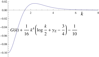
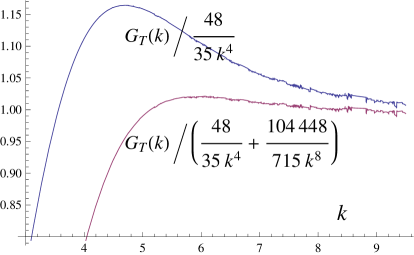
Figure 1: Left panel: Numerically computed finite $T$ part $G_{T}(k)$ of the correlator, the vacuum part (40) is subtracted. Right panel: Check of the analytic expressions (41) for the large-$k$ behavior of $G_{T}(k)$. The constants here were originally determined numerically, only later confirmed analytically.

3 Numerical results for $G(k)$

3.1 The static case $\omega=0$

Comparing Eqs. (23) and (31) and changing from $k\equiv k/(2\pi T)$ back to $k\equiv k/(\pi T)$ one sees that $A(k)=1$ and

$$B(k)=-\textstyle{\frac{1}{16}\,}k^{4}\left[\log\textstyle{\frac{1}{2}\,}k+\gamma_{E}-\textstyle{\frac{3}{4}\,}\right]+\textstyle{\frac{1}{10}\,}+{\cal O}(k^{-4}).$$ (39)

There thus is a diverging vacuum contribution plus a constant term $1/10$. Including this in $G_{\mbox{\scriptsize vac}}$ we write

$$G(k) = G_{\mbox{\scriptsize vac}}(k)+[G(k)-G_{\mbox{\scriptsize vac}}(k)]=G_{\mbox{\scriptsize vac}}(k)+G_{T}(k),$$

$$G_{\mbox{\scriptsize vac}}(k) = -\textstyle{\frac{1}{16}\,}k^{4}\left[\log\textstyle{\frac{1}{2}\,}k+\gamma_{E}-\textstyle{\frac{3}{4}\,}\right]+\textstyle{\frac{1}{10}\,}.$$ (40)

Furthermore, the large-$k$ behavior of $G_{T}$ is

$$G_{T}(k)={48\over 35k^{4}}+{104448\over 715k^{8}}+{\cal O}(k^{-12}).$$ (41)

In the numerical integration of (13) the initial condition is simply $\phi_{h}(1,0,k)=1$, the other solution diverges logarithmically. Because of the $1/(1-z^{4})$ factor the integration is started from $z=1-\epsilon^{\prime}$ ($\epsilon^{\prime}=0.2$), correcting the initial conditions of $\phi_{h}$ and $\dot{\phi}_{h}$ by the expansion (30) (up to $(1-z)^{20}$ was used). Eq. (37) is then evaluated at some $z=\epsilon$ ($\epsilon=0.2$) using the expansions (32) and (34) (up to $z^{40}$ was used). The finite $T$ part obtained after subtracting the vacuum part in (40) is plotted in Fig. 1. The figure also shows how well its large $k$ behavior in Eq. (14) is reproduced. One sees that this expansion converges rapidly, already at $k=6$ the error is $<1\%$. What is important is that there are no terms decreasing more slowly.

Fig. 1 gives the quantities in dimensionless units. If $G_{T}$ and $k$ are in physical units, Fig. 1 plots $G_{T}(k)/(\pi T)^{4}$ vs $k/(\pi T)$.

3.2 The case with $\omega\not=0$

The static correlator $G(r)$ is obtained by Fourier transforming $G(k)$ in the previous subsection, but it may be illuminating to see how the same result is obtained with full $\omega$ dependence, using Eq. (5).

To begin with, from (38) one finds that ($\omega>0$)

$${\rm Im\,}G_{\mbox{\scriptsize vac}}\equiv\rho_{\mbox{\scriptsize vac}}(\omega)={\pi\over 32}(\omega^{2}-k^{2})^{2}\Theta(\omega-k).$$ (42)

Fig. 2 shows how well the numerics approaches this vacuum spectral function. This divergence will be subtracted in what follows.

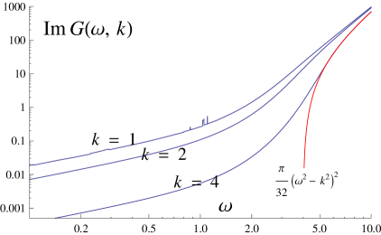
Figure 2: Data for $\rho(\omega)\equiv{\rm Im}G(\omega,k)$ for $k=1,2,4$ plotted vs $\omega$, The approach to the vacuum spectral function (42) is shown by the red curve for $k=4$.

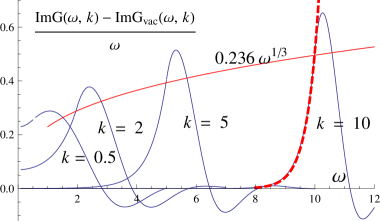
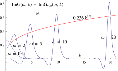
Figure 3: Data for $[\rho(\omega,k)-\rho_{\mbox{\scriptsize vac}}(\omega,k)]/\omega$, $\rho_{\mbox{\scriptsize vac}}=\pi/32\cdot(\omega^{2}-k^{2})^{2}\Theta(\omega-k)$, the left panel plots fixed values of $k$ as a function of $\omega$, the right panel the opposite. The red curve shows the result (43) exactly on the light cone, $\rho(k,k)/k$. The red dotted curve is an exponential fit $0.51e^{2.5(k-10)}$.

After vacuum subtraction one finds that $\rho-\rho_{\mbox{\scriptsize vac}}$ is non-zero essentially close to the light cone. The solution for $\phi$ exactly on the light cone is given by the Hankel function in (29). The Green’s function is evaluated from (37) or directly by computing $2/u\cdot\phi^{\prime}(u)/\phi(0)$ with the result

$$G(k,k)=(1+i\sqrt{3}){\Gamma(1/3)\over 8\cdot 6^{1/3}\Gamma(2/3)}\,k^{4/3}+{\cal O}(1)\approx(0.136092+i\,0.235718)\,k^{4/3}.$$ (43)

In transforming (29) one must remember that there $k\equiv k/(2\pi T)$ while in the numerics $k\equiv k/(\pi T)$. Also note that $\Gamma(\textstyle{\frac{2}{3}\,})\Gamma(\textstyle{\frac{1}{3}\,})=2\pi/\sqrt{3}$. Fig. 3 plots the vacuum-subtracted imaginary part either as a function of $\omega$ for various values of $k$ or as a function of $k$ for various values of $\omega$ and one sees that the analytic form (43) works very well at $\omega=k$ (note that this is not the top of the curves), even down to $k\raise 1.29167pt\hbox{$>$\kern-7.5pt\raise-4.73611pt\hbox{$\sim$}}2$. The left panel of Fig. 3 shows how the decrease off the peak is roughly exponential [6]. For the real part (not shown) the agreement is similar, though the $k^{4/3}$ behavior sets in at somewhat larger values of $k\raise 1.29167pt\hbox{$>$\kern-7.5pt\raise-4.73611pt\hbox{$\sim$}}10$.

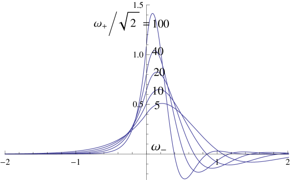
Figure 4: Data for $[\rho(\omega,k)-\rho_{\mbox{\scriptsize vac}}(\omega,k)]/\omega$ when crossing the light cone in a perpendicular direction, i.e., in the direction of $\omega_{-}$, $\omega_{\pm}=(\omega\pm k)/\sqrt{2}$, plotted for increasing values of $\omega_{+}$. Note how the peak gets narrower with increasing $\omega_{+}$, the curves are of the form $k^{1/3}\,F(k^{1/3}\omega_{-}$). The real part has a similar structure, but the positive peak is at $\omega_{-}<0$ and the dips at $\omega_{-}>0$ are deeper.

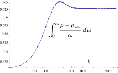
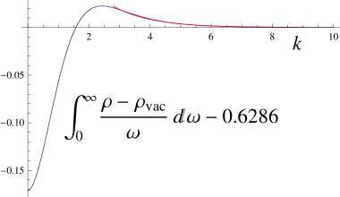
Figure 5: Data for the integral (44) as a function of $k$. The limits for $k\to 0$ and $k\to\infty$ are $3\pi/20$ and $4\pi/20$.The right panel has the numerically obtained asymptotic value $0.6286$ subtracted.

To study in more detail the region around the light cone, Fig. 4 shows the variation when one crosses the light cone perpendicularly to it, in the direction of $\omega_{-}=(\omega-k)/\sqrt{2}$ at fixed $\omega_{+}=(\omega+k)/\sqrt{2}$. One sees that the prediction made after Eq. (29) is confirmed: the quantity in Fig. 4 depends essentially on the combination $k^{1/3}(\omega-k)$, it is of the form $k^{1/3}F(k^{1/3}\omega_{-})$, where $F(0)$ can be read from (43). Thus while the peak height increases, its width decreases. A consequence of this is that the integral over the peak,

$$\int_{0}^{\infty}d\omega\,{\rho(\omega,k)-\rho_{\mbox{\scriptsize vac}}(\omega,k)\over\omega},$$ (44)

approaches a constant at large $k$, see Fig. 5. The accuracy is such that within the range 10…80 the last digit in 0.6286 varies between 3…8. Subtracting this constant one obtains the right panel of Fig. 5. After multiplication by $2/\pi$ this curve is, within numerical accuracy, the same as in the left panel of Fig. 1. One has, along a rather roundabout way on the $k,\omega$ plane, shown that Eqs. (2) and (5) lead to the same result.

That this numerically obtained constant is actually $\pi/5$ can be derived as follows by first deriving its value at $k=0$. A properly subtracted dispersion relation is (at any $k$)

$$G(\omega)-G_{\mbox{\scriptsize vac}}(\omega)-\bigl{[}G(\omega\to\infty)-G_{\mbox{\scriptsize vac}}(\omega\to\infty)\bigr{]}=\int_{-\infty}^{\infty}{d\,\omega^{\prime}\over\pi}{\rho(\omega^{\prime})-\rho_{\mbox{\scriptsize vac}}(\omega^{\prime})\over\omega^{\prime}-\omega}.$$ (45)

For $k=0$ one can work out the $\omega\to\infty$ limit of $G(\omega,k=0)$ exactly as the $k\to\infty$ limit of $G(\omega=0,k)$ was worked out in subsection 2.1, with the result $G(\omega\to\infty)-G_{\mbox{\scriptsize vac}}(\omega\to\infty)=-3/10+{\cal O}(1/\omega^{4})$ [9]. This constant $-3/10$ is the analogue of the constant 1/10 in Eq. (14). If one now takes $\omega=0$ in (45), the LHS leaves just the constant $3/10$ and the RHS is $2/\pi\times$ (44) at $k=0$: the value of (44) at $k=0$ is $3\pi/20$. Since the $k$ dependence has to be the same as that in the static case, Fig. 1, the value of (44) at $k=\infty$ is $4\pi/20$.

4 $G(r)$

4.1 The static case $\omega=0$

To finally get the correlator in coordinate space we have to compute the integral (the normalisation ${\cal L}^{3}/(4\pi G_{5})$ will be appended later)

$$G(r)=\int{d^{3}k\over(2\pi)^{3}}e^{i{\bf k}\cdot{\bf x}}\left[G_{\mbox{\scriptsize vac}}(k)+G_{T}(k)\right].$$ (46)

In the Fourier transform of $G_{\mbox{\scriptsize vac}}$ all terms but the $\log k$ term in (40) are contact terms, proportional to $\delta({\bf x})$ or derivatives thereof, and can be neglected. Using

$$\log k=\int_{0}^{\infty}{dt\over t}\left(e^{-t}-e^{-kt}\right)$$ (47)

the $\log k$ term becomes

$$\int{d^{3}k\over(2\pi)^{3}}e^{i{\bf k}\cdot{\bf x}}G_{\mbox{\scriptsize vac}}(k)=-\infty\,{\rm contact\,\,term}+{1\over 32\pi^{2}r}\int_{0}^{\infty}{dt\over t}\int_{0}^{\infty}dk\,k^{5}\sin(rk)e^{-kt}={15\over 8\pi r^{7}}.$$ (48)

If we introduce ${\cal L}^{3}/(4\pi G_{5})=N_{c}^{2}/(2\pi^{2})$, as is appropriate for ${\cal N}=4$ conformal field theory, and restore physical units by appropriate powers of $z_{h}$, the final result can be written as

$${G(r)\over N_{c}^{2}(\pi T)^{7}}={15\over 16\pi^{3}\bar{r}^{7}}+{1\over 4\pi^{4}\bar{r}}\int_{0}^{\infty}dk\,k\sin(\bar{r}k)G_{T}(k),\quad\bar{r}\equiv\pi Tr.$$ (49)

Comparing with the next-to-leading order computation in SU($N_{c}$) Yang-Mills theory [4] one notes that the leading UV terms are the same if one corrects for an obvious factor of 16. This arises since [3] studies correlators of $F_{\mu\nu}^{a}F_{\mu\nu}^{a}$ while in AdS/CFT duality the scalar couples to the operator $\textstyle{\frac{1}{4}\,}F^{2}$ with the factor $\textstyle{\frac{1}{4}\,}$.

The finite $T$ part of the full result in (49), multiplied by 16, is compared with the NLO computation in [4] in Fig. 6; the leading $1/r^{7}$ terms are the same. One observes that in the finite $T$ part there is a similar region of negative correlator around $\pi Tr=1$, but there is one crucial difference, the QCD result contains terms $\sim(\epsilon+p)/r^{3}$ and $(\epsilon-3p)/r^{3}$ while there are no terms $\sim 1/r^{3}$ nor other terms diverging for $r\to 0$ in the finite $T$ AdS result. The NLO QCD result turns positive at $\pi Tr\approx 2.6$, we do not see this in the AdS result.

The relative magnitudes of the vacuum and finite $T$ parts of (49) are compared in Fig. 7. One sees that the vacuum part dominates for $\pi Tr<1$, the finite $T$ part grows in relative importance for $1<\pi Tr<4$ and for $\pi Tr>4$ both terms essentially cancel each other.

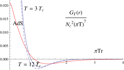
Figure 6: Comparison of the result $G_{T}$ for the finite $T$ part in (49) (multiplied by 16 to get a correlator of $F^{2}$) with the NLO computation in SU($N_{c}$) Yang-Mills theory in [4] for $T=3T_{c}$ and $T=12T_{c}$ (dashed). The right panel shows the large $k$ region. The leading $1/r^{7}$ divergence at small $r$ (not shown) is the same for the two computations.

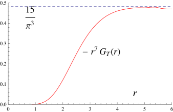
Figure 7: Comparison of the relative magnitudes of the vacuum and finite $T$ parts of (49) (multiplied by 16 to get a correlator of $F^{2}$). Both terms are multiplied by $r^{7}$, $r\equiv\pi Tr$.

4.2 The case with $\omega\not=0$

In this case one can write, from Eq. (5),

$$G(r) = {1\over 2\pi^{2}r}\int_{0}^{\infty}dk\,k\sin(rk)\biggl{[}\int_{-\infty}^{\infty}{d\omega\over\pi}{\rho_{\mbox{\scriptsize vac}}(\omega,k)\over\omega}+\int_{-\infty}^{\infty}{d\omega\over\pi}{\rho(\omega,k)-\rho_{\mbox{\scriptsize vac}}(\omega,k)\over\omega}\biggr{]}$$ (50)

$$= {1\over 2\pi^{2}r}{2\over\pi}\int_{0}^{\infty}dk\,k\sin(rk)\times$$

$$\hskip 60.00009pt\biggl{[}\int_{k}^{\infty}{d\omega\over\omega}{\pi\over 32}(\omega^{2}-k^{2})^{2}e^{-\tau\omega}+\int_{0}^{\infty}d\omega{\rho-\rho_{\mbox{\scriptsize vac}}\over\omega}-0.6286+0.6286\biggr{]}$$

$$= {1\over\pi^{3}r}\biggl{\{}{15\pi^{2}\over 8r^{6}}+\int_{0}^{\infty}dk\,k\sin(rk)\biggl{[}\int_{0}^{\infty}d\omega{\rho-\rho_{\mbox{\scriptsize vac}}\over\omega}-0.6286\biggr{]}\biggr{\}}+{\rm const}\cdot\delta({\bf x}).$$

Here the Fourier transform of the vacuum contribution is computed by introducing a convergence improving factor $e^{-\tau\omega}$. The vacuum integrals over $\omega$ and $k$ can then be done analytically and the limit $\tau\to 0$ leads to the expression in (50) above. Since the square bracket in the integrand in the RHS, after multiplication with $2/\pi$, coincides with $G_{T}(k)$, this result is the same as in (49).

5 $G(\tau,{\bf k}=0)$ and $G(\tau=0,r)$

Various $\tau$ dependent correlators can also be computed using the spectral representation (4). A particularly simple case is the $\tau$ dependent correlator at zero spatial momentum, obtained by summing over spatial volume. Using the spectral representation (4) and the explicit form (42) one has, within the range $0<\tau<1/(2T)$,

$$G(\tau,{\bf k}=0) = \int_{0}^{\infty}d\omega\biggl{[}\textstyle{\frac{1}{32}\,}\omega^{4}+\textstyle{\frac{1}{\pi}\,}(\rho(\omega,0)-\rho_{\mbox{\scriptsize vac}}(\omega,0))\biggr{]}{\cosh[(1-2T\tau)\textstyle{\frac{\pi}{2}\,}\omega]\over\sinh\textstyle{\frac{\pi}{2}\,}\omega}$$ (51)

$$= {3\over 4\pi^{5}}[\zeta(5,T\tau)+\zeta(5,1-T\tau)]+G_{2}(T\tau),$$

where one has noted that in the dimensionless units used here $\beta\omega\to\pi\omega$ and where $G_{2}$ has to be integrated numerically. The integrand is similar to the $k=0.5$ curve in Fig. 3, multiplied by $\omega$. For small $x$,

$$\zeta(5,x)+\zeta(5,1-x)={1\over x^{5}}+2\zeta(5)+30\zeta(7)x^{2}+{\cal O}(x^{4}).$$ (52)

Physical dimensions of $G$ are restored by multiplying by $(\pi T)^{5}$ so that the first term produces the $T$ independent UV divergence $3/(4\tau^{5})$. Again, there are no further divergent terms. One finds that the component $G_{2}$ is numerically insignificant even at $T\tau=\textstyle{\frac{1}{2}\,}$, where it is largest relative to the $\zeta$ function terms.

A more complicated case is $G(\tau,r)$. We give, for completeness, only the part obtained by inserting to (4) the vacuum spectral function (42):

$$G_{\mbox{\scriptsize vac}}(\tau,r)={6\over\pi^{2}r^{8}}\sum_{0}^{\infty}\biggl{\{}{1\over[\pi^{2}(n+T\tau)^{2}/r^{2}+1]^{4}}+{1\over[\pi^{2}(n+1-T\tau)^{2}/r^{2}+1]^{4}}\biggr{\}}.$$ (53)

The sum can be expressed in terms of derivatives of the gamma function, but this is not very illuminating. For equal $\tau$ correlators one has

$$G_{\mbox{\scriptsize vac}}(\tau=0,r)={6\over\pi^{2}r^{8}}\left[\frac{1}{24}r^{4}\text{csch}^{4}(r)+\frac{1}{12}r^{4}\coth^{2}(r)\text{csch}^{2}(r)+\frac{1}{4}r^{3}\coth(r)\text{csch}^{2}(r)+\right.$$

$$\left.\frac{5}{16}r^{2}\text{csch}^{2}(r)+\frac{5}{16}r\coth(r)\right],$$ (54)

where the quantity in the brackets $=1+r^{8}/4725+{\cal O}(r^{10})$. Including the factor $N_{c}^{2}/(2\pi^{2})$ and multiplying by 16 to get correlators of $F^{2}$, the leading singular term $\sim 48N_{c}^{2}/(\pi^{4}r^{8})$ is seen to agree with that in [3].

6 Conclusions

Motivated by needs of lattice work [1], we have in this article computed the $r$ dependence of the $\tau$ integrated finite temperature correlator $\langle F^{2}(\tau,{\bf x})F^{2}(0,{\bf 0})\rangle$ and compared it with the same in SU($N_{c}$) Yang-Mills theory [4]. Our computation based on AdS/CFT duality applies to ${\cal N}=4$ conformal strongly coupled theory and there is no reason for the results to coincide. The leading UV vacuum part $\sim 1/r^{7}$, $r\to 0$, coincides since it is independent of the coupling. However, the leading finite $T$ parts differ, in the QCD-like case there are terms $\sim(\epsilon+p)/r^{3}$ and $\sim(\epsilon-3p)/r^{3}$, while for AdS/CFT we find no terms $\sim T^{4}/r^{3}$ nor other finite $T$ terms diverging for $r\to 0$. $G_{T}$ is just some function $G_{T}(\pi Tr)$, finite for $r\to 0$. In the range $r\sim{\rm few}\,\,1/(\pi T)$ both finite $T$ correlators are negative. For $r>4/(\pi T))$ the AdS finite $T$ correlator essentially cancels the vacuum one.

The computation was carried out both taking $\omega=0$ from the outset, but also by integrating the weighted spectral function over $\omega$. These results coincide due to observed structure near the light cone, $\omega=k$. It would be interesting to have analytic control of observed scaling as a function of $k^{1/3}(\omega-k)$.

An obvious task for the future would be carrying out a similar computation for holographic QCD models [11, 12] breaking conformal invariance. This will also shed light on the difference between $\langle F^{2}(x)F^{2}(0)\rangle$ and $\langle F^{2}(x)\tilde{F}^{2}(0)\rangle$ correlators.

Acknowledgements. KK thanks J. Alanen, Sean Nowling, Aleksi Vuorinen and, in particular, Jorge Casalderrey-Solana for discussions and advice. The work of MV has been supported by Academy of Finland, contract no. 128792.

References

- [1] H. B. Meyer, “Energy-momentum tensor correlators and spectral functions,” JHEP 0808, 031 (2008) [arXiv:0806.3914 [hep-lat]].
- [2] N. Iqbal and H. B. Meyer, “Spatial correlators in strongly coupled plasmas,” JHEP 0911, 029 (2009) [arXiv:0909.0582 [hep-lat]].
- [3] M. Laine, M. Vepsalainen and A. Vuorinen, “Ultraviolet asymptotics of scalar and pseudoscalar correlators in hot Yang-Mills theory,” JHEP 1010, 010 (2010) [arXiv:1008.3263 [hep-ph]].
- [4] M. Laine, M. Vepsalainen and A. Vuorinen, “Intermediate distance correlators in hot Yang-Mills theory,” arXiv:1011.4439 [hep-ph].
- [5] G. Policastro and A. Starinets, “On the absorption by near-extremal black branes,” Nucl. Phys. B 610, 117 (2001) [arXiv:hep-th/0104065].
- [6] D. T. Son and A. O. Starinets, “Minkowski-space correlators in AdS/CFT correspondence: Recipe and applications,” JHEP 0209, 042 (2002) [arXiv:hep-th/0205051].
- [7] P. K. Kovtun and A. O. Starinets, “Quasinormal modes and holography,” Phys. Rev. D 72, 086009 (2005) [arXiv:hep-th/0506184].
- [8] P. Kovtun and A. Starinets, “Thermal spectral functions of strongly coupled N = 4 supersymmetric Yang-Mills theory,” Phys. Rev. Lett. 96, 131601 (2006) [arXiv:hep-th/0602059].
- [9] P. Romatschke and D. T. Son, “Spectral sum rules for the quark-gluon plasma,” Phys. Rev. D 80, 065021 (2009) [arXiv:0903.3946 [hep-ph]].
- [10] F.W.J. Olver, Asymptotics and special functions, A.K.Peters, Wellesley, 1997.
- [11] U. Gursoy and E. Kiritsis, “Exploring improved holographic theories for QCD: Part I,” JHEP 0802, 032 (2008) [arXiv:0707.1324 [hep-th]].
- [12] U. Gursoy, E. Kiritsis and F. Nitti, “Exploring improved holographic theories for QCD: Part II,” JHEP 0802, 019 (2008) [arXiv:0707.1349 [hep-th]].